D.A. Jones
Hydrology and Earth System Sciences, 7(5), 642651 (2003) © EGU
Use of several indices of event severity for floods and droughts
D.A. Jones
Centre for Ecology and Hydrology, Wallingford, Oxfordshire, OX10 8BB, UK
Email: [email protected]
Abstract
An examination is made of the true return periods associated with certain types of composite indices for the rareness of events. In particular, return periods are evaluated separately for several different ways of describing how bad an event was, and the composite index, or apparent return period, is defined as the largest of these component return periods. Such apparent return periods give an incorrect indication of how often a larger value for the composite index will occur. Simulations are used to study the relationship between the true and apparent return periods for some simple cases, and an assessment is made of the extent of the error made if the apparent return period is used directly. A simple practical procedure is described for dealing with real datasets without model-fitting, and this is assessed using further simulations. An example is given relating to a possible flood situation where a composite index is constructed as the largest of the return periods of high rainfall-accumulations over a number of durations.
Keywords: drought severity index, composite index, event severity, return period
Introduction
The first problem to be faced when trying to assess the rareness of hydrological events, such as floods or droughts, is that of defining the particular set of events of interest, or more specifically, defining those qualities of floods or droughts which cause most difficulties for those affected. Any treatment of this problem needs to be linked closely to the reason why the question is being asked. Different approaches are likely to be necessary depending on whether the background to the question is a formal one, such as when designing new water-resources infrastructure, or an informal one, such as when a notable event has occurred and the general public ask how often can we expect something like this?. The major difficulty is that there is no unique way of characterising the size of a flood or drought. A meaningful assessment of the rareness of an event can only be obtained by tailoring a measure (or measures) of how bad conditions are, defining the direction (or directions) in which conditions are worse, and then evaluating the probability of observing an event which is as bad, or worse than, that actually observed. This can be an extremely difficult task, since the practical effects of extreme deficits and excesses of water in the environment will vary with:
(i) the locations which are affected;
(ii) the geographical spread of the region affected, since many sites being affected will be disproportionately worse than just a few;
(iii) the duration of the extreme period;
(iv) temporal variations within a period of extremity; (v) the time since the preceding period of extremity;
and so on. Similar lists of aspects of extreme events that need to be considered have been provided by, among others, Hoyt (1942), Ibbitt et al.(1997) and Ward and Robinson (2000, p50).
When return periods are evaluated for several indices each measuring different aspects of an event, the largest of these may conveniently be called the apparent return period. This then becomes just another way of measuring how extreme an event has been and, although the words return period are used in the name, it is important not to treat the values quoted as if they were return periods for the event. If apparent return periods are calculated in the same way for events in a long period of time, a given value for the apparent return period, say T years, will occur rather more frequently than 1 in T years. The actual frequency of occurrence will be called the true return period.
While taking the largest of several return periods can be misleading, it may sometimes be used in practice with the underlying knowledge that the apparent return period is incorrect but conservative (unfortunately there are few practical cases where this does err on the side of safety). In more general circumstances, there can be attractions in using an approach of taking several quantities measured on disparate scales and converting them to a common probability or return-period scale before combining them into a single composite index of severity. The results in this paper indicate that, in practically useful cases, reliable estimates of the true return periods of such composite indices can be obtained by simple data analyses.
Evaluating the rareness of several measures of event severity is something that may be undertaken in the initial stages of more formal analyses. To summarise briefly, possibilities for these more formal analyses include:
(a) modelling of a water resource system in terms of one or more reservoirs, and evaluating the ability to meet demand for water supply for domestic or irrigation usage;
(b) construction of a single response variable representing the consequences of conditions at a number of sites, with the rareness of the response variable being derived by some type of joint probability analysis;
(c) detailed analysis of a water supply system or flood detention reservoir to identify a so-called critical duration of events for the system, leading to selection of a particular measure of event size from the many possible;
(d) formal combination of several measures of event severity, by standardising individual measures and averaging, evaluation of the new measure for the historical record, followed by a formal analysis of the derived series to determine event rareness.
The next section of this paper gives results for some simple types of application where multiple indices of event severity
are often quoted and where certain assumptions allow exact results to be obtained by a combination of analysis and random simulations. A later section uses a real dataset to illustrate methods of analysis to evaluate the actual rareness of events identified from the worst of several indices of event severity.
Analysis of a simple case
BACKGROUND
Suppose that there is a need to assess the severity of an ongoing drought and that this is to be done using a record of monthly rainfalls. Suppose that a calendar month, say September, has just finished and data for this month and previous months are available. Then the value, x1, of the latest September rainfall-total can be referred to the distribution of the random variable X1, where this represents how September rainfalls vary from year to year. Specifically, the record of past September rainfalls enables an estimate to be obtained for
1 1 1 11 Pr X x F x
p d . (1)
For the analysis of this section, errors in estimating this and similar quantities will be ignored and it is assumed that the corresponding distribution functions are fully known. Thus, across a typical set of years, there is a probability p1 that the September rainfall would be equal to or more extreme (lower) than current conditions. Alternatively, the return period, r1 = p11, can be used as the measure of event
severity to indicate that only 1 in r1 years would contain similar or worse (drier) conditions for the September rainfall. A set of similar analyses can be made which examine rainfall-totals over successively longer durations. In particular, if (xn, xn1, ...., x2, x1) are the values of monthly rainfall for the n months ending with x1 being value for the latest September, then the n-month total is
n
n
x
x
x
s
2
1 , (2)
for which there is a corresponding random variable, Sn, defined in terms of the random variables X1 representing rainfalls in individual calendar months by
n
n X X X
S
2
1 . (3)
Then the probability and return period associated with the n-month total are
n n n nn S s F s
p Pr d , 1
n
n p
D.A. Jones
Note that the notation here (in particular the backward-indexing of the monthly values) has been chosen so that Eqn. 3 accords with the expressions used in the theory of random walks (Feller, 1971).
Taken individually, any particular return period, rn, is an
index of the severity of conditions up to the current time. It has a valid interpretation that for only 1 in rn years will this
index, if recalculated at the end of each September, equal or exceed its current value (rn). In applications where there
is no one duration, n, that is obviously most appropriate, then the results for several durations might well be quoted. Suppose that the return periods for rainfall totals of durations n = 1, 2, ..., N are available. Then, given that these measure event-severity on the same scale for all durations, it is natural to think of combining them in some way. The most immediately appealing way is to determine
Napp
N r r r
r max 1, 2,, , (5)
where app N
r denotes the apparent return period of conditions up to duration N. Of course, the quantity rNapp does not have
a correct interpretation as the return period of this new index of event-severity. The main purpose of this section is to examine the true return period rNtrueof the event
^
app`
N app
N r
R t in order to provide a guide to how large the discrepancy between app
N
r and rNtrue can be. This is undertaken in a situation which is not obscured by other problems such as the effects of estimating the distribution functions Fn for n = 1,..., N. Here
app N
R denotes the random variable corresponding to evaluating rNapp in exactly the same
way in other (past or future) years with September as the final calendar month.
The above may be put in a practical context by noting that, excluding the step of using the largest return periods across several durations, the approach is much used in the UK in the context of monthly and longer duration total rainfalls. Specifically, the Met Office routinely makes use of the marginal distributions of n-month totals beginning (or equivalently, ending) in a specific month following work by Tabony (1977). The method has been applied to periods of high rainfall as well as to droughts, given the obvious changes to examine the upper rather than the lower tails of the distributions: see Dale and Jones (2001) for example. In contrast, studies of river flooding have usually used a much shorter base time-step than one-month and, because of this, probabilities and return periods are evaluated on a different basis. For example, if a single day of high river flow has occurred on October 15, the question asked is how often will this flow be exceeded at any time of year?, not on how many October 15s will the flow be exceeded?. Here the n-day totals would be referred to the distribution
of the yearly maximum of n-day totals within the year, instead of to the distribution of n-day totals ending at a given time point. The effect on the formulae above is to replace the distribution functions Fn with different ones. As an example, Jakob et al. (2001) use this annual-maximum basis to evaluate the rareness of high rainfalls leading up to a certain widespread flooding event over durations of 1, 7, 15, 30 and 60 days. Once again, the potential to be misled by the use of several indices of event severity exists: the effect for analyses based on distributions for annual extremes is likely to be similar but different in detail from those based on distributions targeted at a fixed time of year. The results in the present section have been evaluated for the fixed-time-of-year case because they are determined by fewer parameters and assumptions than the alternative case. While it would be possible to extend the analyses here to include cases where the durations included in the set of indices are not equally spaced, this has not been undertaken as the results are intended only as a guide to the possible effects of using the worst of several indices.
SIMULATION RESULTS
The results presented in Figs. 1 and 2 and Table 1 apply to the following situation. It is assumed that the individual values X1, X2,..., XN in a sequence of calendar months are independent and have the same distribution apart possibly from a change in location. The effect of any change in location is, of course, removed by the calculation of the probabilities pn according to the marginal distributions of the totals Sn: this would not apply in the annual maximum case. Similarly, the results are not affected by the scale of distributions of the individual values (but the scale parameter must be the same for each). Results have been calculated for a small number of different distributions for the monthly values: these distributions have been selected because explicit results are known for the distributions of the totals Sn. For some distributions, the straightforward simulation of the distribution of app
N
0 2 4
200 100
50 10
2
Apparent rareness
0
2
4
200
100
50
10
2
1.1
1.01
True rareness
LE N UE C 1:1
0 2 4
200 100
50 10
2
Apparent rareness
0
2
4
200
100
50
10
2
1.1
1.01
True rareness
2
4
8 16 32 64 128
1:1
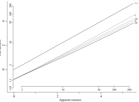
Fig. 1. Relation of true rareness to apparent rareness when N = 8, for the cases: Cauchy (C), upper tail of the Exponential (UE), Normal (N) and lower tail of the Exponential (LE). Outer axes use the Gumbel scale, while the inner axes show return periods in years.
D.A. Jones
in this case two sets of results have been derived, one for the lower tail of the distribution (looking for sequences of low values) and one for the upper tail, in which case the calculations are revised to be appropriate to looking at sequences of high values. This set of distributions was selected to give a range of behaviour for the length of the tail of the distribution from short (the lower tail of Exponential), through Normal and the upper tail of the Exponential, to long (Cauchy). The Cauchy distribution may be considered unrealistic for practical applications because it is so long-tailed that the mean and higher moments do not exist: however, it is included because it is both (i) one of the few distributions for which the required explicit results are available and (ii) an instance of a distribution with power-like tails to the density function. The availability of explicit results for the distributions of the cumulative totals Sn means
that the simulations are straightforward and closely match the situation for which some theoretical results are available, as discussed in the next subsection. It would of course be possible to implement simulation procedures in which the distributions of Sn are estimated as part of the overall procedure, but at the expense of extra computations and less clarity.
Figure 1 shows how the distribution of the individual values Xi affects the relationship of the true rareness (return period), rNtrue, to the apparent rareness,
app N
r , for one choice of N, the largest duration included in the set of severity measures. Similar results are found as N varies. For visualisation of the results, the return periods are shown on the usual Gumbel scale simply because this is a convenient choice. One particular point to note from Fig. 1 is that the curves seem to pass through the same point when the apparent rareness is a return period of two years. This is a special case of the more general problem here, but one for which some limited theoretical results are available: these
are outlined in the following subsection. The special case relates to the question of how often at least one of S1,...,SN will all lie on the extreme side of their respective medians: this will clearly happen rather more often than one out of two cases. Although it appears that the lines in Fig. 1 cross, this is misleading: the curve for the Cauchy distribution is highest on both sides of app 2,
N
r while the ordering of the other three is reversed on passing through the intersection. In addition, the curves do not in fact intersect at the same point: see the subsection on theoretical results.
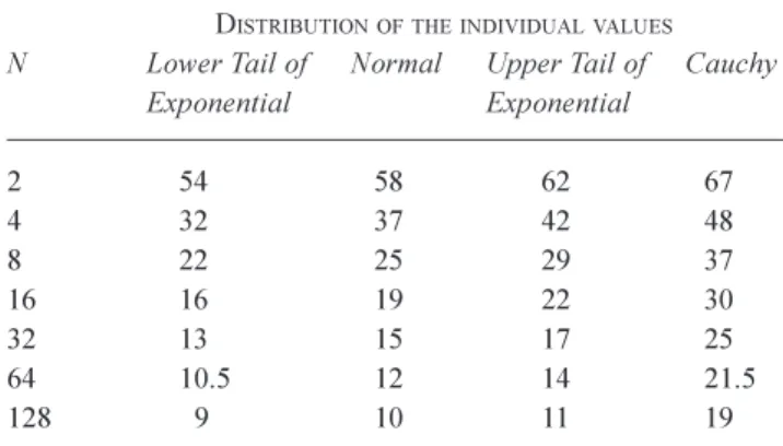
Figure 2 illustrates the effect of changing N, the number of indices of severity being considered: once again the results are similar for other distributions, so only a single example is given. As expected, the true return period corresponding to a fixed apparent rareness decreases rapidly as N increases. Table 1 gives a summary of how the true rareness can vary when the apparent rareness is a return period of 100 years, depending on the distribution of the individual values and on the number of indices of severity being considered. It is important to remember that these results apply to the case where the indices relate to totals or averages over sequentially increasing durations and where the individual values are statistically independent.
RELATED THEORETICAL RESULTS
It was noted above that the curves in Fig. 1 seem to have the same true rareness for outcomes having an apparent rareness of two years. This is a special case for which some theoretical results can be derived, from the theory of random walks, which partly back this result. Having rNapp 2 means
that ri 2 for all of the individual durations, and hence
that pi !12 (i 1,,N). Now 2 1
!
i
p corresponds to si
being larger than the median, mi of the distribution of Si. Hence
; 1, , . Pr 1 , 2 Pr 1 2 Pr N i m S R R S i i app N app N ! t (6)The underlying theoretical results that are available relate to distributions of the individual values, Xi, which are symmetric and continuous, as is the case for the Normal and Cauchy distributions. For these distributions, a shift in location can be made without affecting the results in such a way that the median of Xi is zero, which then means that the
median of Si is also zero. Then results stated by Feller (1971: Section XII.7, Theorem 4 and Section XII.8, after Lemma 1) and by Feller (1970: Eqn. II.12.5) show that, for all symmetric and continuous distributions,
2 1 2 2 .Pr Napp 2N
N N R ¸¸ ¹ · ¨¨ © § t (7)
Table 1. The true return period when the apparent return period is 100, showing how this varies with the distribution of individual values and with
N
, the number of indices of severityDISTRIBUTIONOFTHEINDIVIDUALVALUES
N Lower Tail of Normal Upper Tail of Cauchy Exponential Exponential
2 54 58 6 2 6 7
4 32 37 42 48
8 22 25 29 37
1616 19 22 30
32 13 15 17 25
64 10.5 12 14 21.5
Hence, in these cases, the true return period of observing an apparent return period of 2 or more is
.
2
2
1
1 2¿
¾
½
¯
®
¸¸
¹
·
¨¨
©
§
N true NN
N
r
(8)For example, N = 1,2,3 gives 2,85,1611
true N
r respectively.
An approximate formula for rNtrue can be derived from an asymptotic expansion for large N using Stirlings Formula (Feller, 1970: Eqns. II.9.1, III.2.4), which gives
. 1 1 1 ¿ ¾ ½ ¯ ® | N rNtrue
S
(9)
This theoretical result confirms that the curves in Fig. 1 do pass through the same point when the apparent rareness is a return period of 2 whenever the distribution of individual values is symmetric and continuous. The simulation results for the non-symmetric exponential case confirm that the above result does not hold exactly for other distributions. For example, for N = 2, true 1.6
N
r for symmetric
distributions, while the simulation results give
5888 . 1
true N
r for both the lower and upper tails of the Exponential distribution. As noted earlier, the number of samples in the simulations was extended to ensure that the values quoted here are correct to the number of decimal places given. When N = 3,, true 1.4545
N
r for symmetric
distributions, while the simulation results give
4429 . 1 , 4439 . 1 true N
r for the lower and upper tails of the
Exponential distribution respectively. While these results for the Exponential distribution are rather close to those for symmetric distributions, it is not clear if this is generally true.
Given that they seem to be approximately valid across a range of distributions, Eqns. 8 or 9 can be used to provide answers to two slightly different questions. The first is based on the idea of equivalent number of independent samples denoted by Ne. The combined index of severity is based on the most extreme of N dependent indices, but one might wonder what the value of Ne would be such that the most extreme of Ne independent indices would have the same
true rareness as the dependent case, at least when the apparent rareness is 2 years. For Ne = M independent indices,
the true rareness of an apparent return period of 2 years is given by
^
`
12
1 M
true M
r , (10)
and with Eqn. 9 this gives, for large N,
/ 2log2log N
Ne | S . (11)
The second question asks whether a sequence of durations
^ `
Ni can be found such that the curves in a new version of Fig. 2 would be equally spaced. This can be achieved with a sequence^ `
Ni which behaves like^
1`
1
2
log
2
exp
|
aii
e
N
S
, (12)for large i. Here a is a positive parameter controlling the spacing of the lines.
Practical analyses for real data
In a limited number of practical applications the results provided in the first section of this paper may be enough to give an approximate idea of the true return period where an apparent return period is derived as the maximum of several return periods calculated for durations which are multiples of a common time-step, provided that the totals at the common time-step can be treated as independent. While the number of component indices used has a strong effect, the effect of the distribution of the underlying variables is rather less important. For example, the results in Fig. 2 and Table 1 should provide adequate guidance for application to monthly rainfalls in the UK. In other cases, it would be possible to devise simulation experiments that more closely match the specifics of a particular application in terms of the details of the component indices and the statistical dependence of the underlying variables. However, given that only an informal assessment of rarity is being undertaken, there may be too much work involved in constructing the simulations and in statistical modelling of the underlying variables.
D.A. Jones
typically not available when considering results published by others.
An outline of the simple procedure when applied to return periods for multiple durations, assessed for a fixed time of year, is as follows.
(i) For each year in the dataset, calculate the totals for each duration finishing at the required point in the calendar year. Count the total for a given duration as missing if this would require data from before the start of record.
(ii) Treating each duration separately, estimate the return periods for the totals for each year. This is done by ranking the set of duration totals and assigning a notional probability of i/(n + 1) to an equal or worse total: here n is the number of years for which totals of the given duration are available and i is the rank of the total for the given year in the set of totals. The procedure can work with these probabilities, or with corresponding values for return periods.
(iii) Treating each year separately, calculate the combined index for that year by taking the worst probability or return period across the values calculated for the different durations. This creates the set of apparent return periods, either directly or indirectly via the probabilities. Where no value for a particular duration is available because the total could not be formed at step (i), this is ignored and the combined index for the year is calculated for the reduced set of durations. (iv) Estimate the true return periods for the apparent return period previously calculated for each year. The estimated true return period for a given year is found by assigning a notional probability of i/(n + 1) to an equal or worse value of the apparent return period: here n is the number of years for which apparent return periods are available and i is the number of years having an apparent return period equal to or higher than that assigned to a given year. The estimated return period would be the reciprocal of this probability.
(v) Create a plot of the estimated true return periods against the apparent return periods, using the Gumbel reduced variate scale for both axes. Use judgement, based on the figures in this paper or based on other simulations, to draw a line representing the required relationship of the true to the apparent return periods. The line should be generally guided by the points corresponding to the lower to medium apparent return periods, with the points for the two or three highest apparent return periods being heavily discounted.
Some simulation results that support the above approach
are given below. A summary of the approach is that it uses the available dataset in two essentially distinct steps. Firstly, yearly values for several indices of severity are established by performing a simple frequency analysis for each index separately. Then, having constructed yearly values of the composite index, a further simple frequency analysis is performed. This double-use of the dataset may be worrying, but it appears from the simulation results that the overall procedure is basically sound. The treatment of incomplete duration-totals at the beginning of the record (in steps (i) and (iii) above) was specified with a particular application in mind, in order to include use of as much data as possible: other specifications may be more appropriate if the composite indices calculated for the initial year or years are thought to be too poorly determined. The simulations reported here adopt the treatment of the initial years as set out above, rather than including extra values before the notional start of record in order that all durations-totals should be complete.
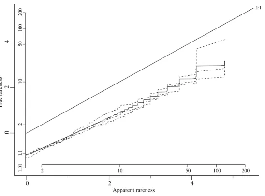
Fig. 3. Relation of true rareness to apparent rareness for the simple analysis procedure. Composite index for droughts of simulated rainfall over 1 to 14 months. Full line shows the true rareness derived from extensive simulations; dashed lines show typical estimates of the true rareness using single blocks of 121 years of data. Outer axes use the Gumbel scale, while the inner axes show return periods in years.
Fig. 4. Relation of true rareness to apparent rareness for the simple analysis procedure. Composite indices for high rainfalls over two different sets of durations. The full and dashed lines show results for 5 and 16 durations respectively (sets (a) and (b) in the text) for a 149 year record at Armagh. Outer axes use the Gumbel scale, while the inner axes show return periods in years.
0 2 4
200 100
50 10
2
Apparent rareness
0
2
4
200
100
50
10
2
1.1
1.01
True rareness
1:1
0 2 4
200 100
50 10
2
Apparent rareness
0
2
4
200
100
50
10
2
1.1
1.01
True rareness
D.A. Jones
the required values provided that allowance is made for the poor estimation at the highest return periods.
The major difference between the results in Fig. 3 and the earlier plots is the presence of steps in the graphs. These arise from the use of the simple frequency analysis step to determine the return periods attributed to the totals of different durations: in most cases the three highest return periods that are calculated are 122, 61 and 40.7 years, although for some longer durations these are slightly modified to 121, 60.5 and 40.3 years. Thus the highest apparent return periods that are calculated within the procedure are restricted to these values. The analysis of a given dataset will usually contain cases where the same apparent return period is attributed to different years and, in particular, the worst 1-month, 2-month, 3-month, etc. totals will often occur in different years and each of these years will be given an apparent return period (for the combined index) of 122 years. In the present context, it is the lower edge of the stepped line that is most relevant in determining the true return period.
The simple analysis procedure can be adapted to a range of circumstances and Fig. 4 shows some results derived for a real set of daily rainfalls in a case where the composite index relates to high rainfalls assessed using annual maximum rainfall-totals over different durations. A record of 149 years of daily rainfall was available for Armagh in Northern Ireland. This was used to assess the true return period where a composite index (apparent return period) for a given year is constructed by finding, for each duration length, the return period of the largest total over that duration terminating within that (calendar) year, and then taking the largest of these. Fig. 4 shows results for two different sets of durations:
set (a): 1, 7, 15, 30, 60 days;
set (b): 1, 2, 3, 5, 7, 10, 15, 20, 30, 60, 90, 120, 150, 180, 210 and 240 days.
The first set corresponds to the durations explicitly considered by Jakob et al. (2001), while the second is included to show the effect of using a more extensive set of component indices. It is not to be expected that the results for these sets of 5 and 16 durations would be similar to those given in Fig. 2 for N = 5 or 16, because the durations here are not equally spaced.
Relation to other work
The present study examines the effect of taking the maximum of a number of related quantities as the variable of most interest. Here the quantities are the totals or averages over varying durations of a set of underlying measurements. Certain other studies have looked at slightly different but
related problems. For example, Dales and Reed (1989) looked at the effect of taking the largest rainfall recorded at any of a collection of raingauges in a spatial region as a measure of event-size, comparing this to the result that would be obtained using raingauges individually. In the context of annual maxima of averages over a fixed duration, Dwyer and Reed (1994, 1995) looked at the effect of either considering only time-periods which abut each other on a regular basis, or allowing the time-periods to overlap. They looked at quantifying the effect of taking the maximum over a more extensive set of quantities, using overlapping intervals, compared with abutting intervals.
Conclusion
It is clear that it is, in principle, incorrect to assess the overall rarity of a flood or drought event by computing return periods for several different measures of event severity and quoting the largest of these. This paper has indicated the extent that such apparent return periods can be wrong. Nevertheless, the approach has some appeal in constructing an overall index of severity, in that it treats each of the component indices on a common scale by converting them into probabilities or return periods. A practical procedure for a two-pass data analysis has been outlined and this has been shown to perform reasonably in providing a good assessment of the true return period of a composite index.
The practical approach outlined in this paper is applicable to a wide range of circumstances. While the example described here was based on rainfall at a single site, it is clear that data-series of regional-average rainfall could equally well be used. In general, an overall index of event severity might be constructed by taking the largest of the return periods estimated separately for many sites within a region, or for sub-areas within an overall region, for different sets of accumulation-periods and for different underlying quantities. It is clear that the practical approach involving double-use of the data, as outlined here, can be readily adapted to provide estimates of the true return-periods of such composite indices.
Acknowledgement
References
Dale, M. and Jones, R., 2001. How unusual were the meteorological conditions during October-November 2000?. In To what degree can the October/November 2000 flood events be attributed to climate change? DEFRA FD2304 Technical Report, CEH Wallingford and the Met Office. 4960. (URL:http://www.defra.gov.uk/science/project_data/ DocumentLibrary/FD2304/FD2304_461_FRP.pdf)
Dales, M.Y. and Reed, D.W., 1989. Regional flood and storm hazard assessment. Report No. 102, Institute of Hydrology, Wallingford, UK.
Dwyer, I.J. and Reed, D.W., 1994. Effective fractal dimension and corrections to the mean of annual maxima. J. Hydrol., 157,
1334.
Dwyer, I.J. and Reed, D.W., 1995. Allowance for discretization in hydrological and environmental risk estimation. Report No.123, Institute of Hydrology, Wallingford, UK.
Feller, W., 1970. An Introduction to Probability Theory and its Applications, Volume I (3rd Edition, Revised Printing). Wiley, New York, USA.
Feller, W., 1971. An Introduction to Probability Theory and its Applications, Volume II (2nd Edition).Wiley, New York, USA. Hoyt, W.G., 1942. Droughts. In: Hydrology, O.E. Meinzer (Ed.), Chapter XII, 579-591, McGraw-Hill, New York (reprinted 1949, Dover Publications, New York, USA).
Ibbitt, R., Woods, R. and McKerchar, A., 1997. Hydrological processes of extreme events. In: Floods and Droughts, the New Zealand Experience, M.O. Mosley and C.P. Pearson (Eds.). New Zealand Hydrological Society, Wellington North, New Zealand. 1528.
Jakob, D., Lamb, R. and Prudhomme, C., 2001. How unusual were the October-November rainfall and river-flows at target sites?. In: To what degree can the October/November 2000 flood events be attributed to climate change? DEFRA FD2304 Technical Report, CEH Wallingford and the Met Office, 6177. (URL:http://www.defra.gov.uk/science/project_data/ DocumentLibrary/FD2304/FD2304_461_FRP.pdf)
Tabony, R.C., 1977. The variability of long-duration rainfall over Great Britain. Meteorological Office Scientific Paper No.37. Ward, R.C. and Robinson, M., 2000. Principles of Hydrology.