Hydrol. Earth Syst. Sci., 17, 1715–1732, 2013 www.hydrol-earth-syst-sci.net/17/1715/2013/ doi:10.5194/hess-17-1715-2013
© Author(s) 2013. CC Attribution 3.0 License.
Geoscientiic
Geoscientiic
Hydrology and
Earth System
Sciences
Open Access
Hydrological drought across the world:
impact of climate and physical catchment structure
H. A. J. Van Lanen1, N. Wanders1,2, L. M. Tallaksen3, and A. F. Van Loon1
1Hydrology and Quantitative Water Management Group, Centre for Water and Climate, Wageningen University,
Wageningen, the Netherlands
2Department of Physical Geography, Faculty of Geosciences, Utrecht University, Utrecht, the Netherlands 3Department of Geosciences, University of Oslo, Oslo, Norway
Correspondence to:H. A. J. Van Lanen ([email protected])
Received: 30 September 2012 – Published in Hydrol. Earth Syst. Sci. Discuss.: 30 October 2012 Revised: 28 March 2013 – Accepted: 3 April 2013 – Published: 2 May 2013
Abstract. Large-scale hydrological drought studies have
demonstrated spatial and temporal patterns in observed trends, and considerable difference exists among global hy-drological models in their ability to reproduce these patterns. In this study a controlled modeling experiment has been set up to systematically explore the role of climate and physical catchment structure (soils and groundwater systems) to bet-ter understand underlying drought-generating mechanisms. Daily climate data (1958–2001) of 1495 grid cells across the world were selected that represent K¨oppen–Geiger ma-jor climate types. These data were fed into a conceptual hy-drological model. Nine realizations of physical catchment structure were defined for each grid cell, i.e., three soils with different soil moisture supply capacity and three groundwa-ter systems (quickly, ingroundwa-termediately and slowly responding). Hydrological drought characteristics (number, duration and standardized deficit volume) were identified from time se-ries of daily discharge. Summary statistics showed that the equatorial and temperate climate types (A- and C-climates) had about twice as many drought events as the arid and po-lar types (B- and E-climates), and the durations of more ex-treme droughts were about half the length. Selected soils un-der permanent grassland were found to have a minor effect on hydrological drought characteristics, whereas groundwa-ter systems had major impact. Groundwagroundwa-ter systems strongly controlled the hydrological drought characteristics of all cli-mate types, but particularly those of the wetter A-, C- and D-climates because of higher recharge. The median num-ber of droughts for quickly responding groundwater systems was about three times higher than for slowly responding
sys-tems. Groundwater systems substantially affected the dura-tion, particularly of the more extreme drought events. Bi-variate probability distributions of drought duration and stan-dardized deficit for combinations of K¨oppen–Geiger climate, soil and groundwater system showed that the responsiveness of the groundwater system is as important as climate for hy-drological drought development. This urges for an improve-ment of subsurface modules in global hydrological models to be more useful for water resources assessments. A foreseen higher spatial resolution in large-scale models would enable a better hydrogeological parameterization and thus inclusion of lateral flow.
1 Introduction
12 million people (UN, 2011). Droughts in developing coun-tries may cause fatalities, which does not happen in pros-perous countries. However, in Europe almost 80 000 people died due to associated heat waves and forest fires over the period 1998–2009. Overall losses were estimated to be as high as C 4940 billion over the same period (EEA, 2010). Likely, drought will worsen in many parts of the world be-cause of climate change (e.g., Bates et al., 2008; Seneviratne et al., 2012). Moreover, vulnerability will increase in numer-ous regions as a response to population growth and, thus, higher demand for water. Water security and associated food supply, in particular under extreme conditions, are at stake (e.g., Falkenmark et al., 2009; WWDR, 2009; Gerten et al., 2011). Large-scale drought can also have a large impact on ecosystems. The 2010 Amazon drought showed that repeated drought may largely influence tropical forests that can shift from buffering a CO2increase into accelerating it, which can
have important decadal-scale impacts on the global carbon cycle (Lewis et al., 2011).
Drought differs from other hazards in several ways. It de-velops slowly and usually over large areas (transnational), mostly resulting from a prolonged period (from months to years) of below-normal precipitation, and drought can oc-cur nearly anywhere on the globe. Lack of precipitation combined with higher evaporation rates propagates through the hydrological cycle from its origin as a meteorological drought into soil moisture depletion to the point where crops or terrestrial ecosystems are impacted, and eventually into a hydrological drought (e.g., Wilhite, 2000; Tallaksen and Van Lanen, 2004; Mishra and Singh, 2010). Hydrological drought refers to a prolonged period with below-normal wa-ter availability in rivers and streams, and lakes, or ground-water bodies due to natural causes. The different types of droughts have each their own specific spatiotemporal char-acteristics (e.g., Peters et al., 2006; Tallaksen et al., 2009). From an impact point of view, it is important to distinguish between the different types of drought and to realize that hydrological drought indicators cannot be straightforwardly derived from meteorological drought indicators (e.g., Peters et al., 2003; Wanders et al., 2010). Understanding different types of drought, including their controlling mechanisms, is of uttermost importance for the management of water re-sources, where key information on hydrological drought is essential for water resources assessments.
Recently, several large-scale studies have been carried out to investigate drought at global or continental scales for present and future climate (e.g., Andreadis et al., 2005; Sheffield and Wood, 2008a, b; Shukla and Wood, 2008; Sheffield et al., 2009, 2012; Dai, 2011, 2013; Hannaford et al., 2010; Prudhomme et al., 2011; Stahl et al., 2011; Corzo Perez et al., 2011; Wehner et al., 2011; Van Huijgevoort et al., 2012). In these studies droughts were derived from time series simulated with large-scale models (e.g., general circu-lation models (GCMs), regional circucircu-lation models (RCMs), land surface models (LSMs), global hydrological models,
(GHMs)), usually tested against documented sources or river flow data (e.g., D¨oll et al., 2003; Hannah et al., 2010). Other large-scale studies have examined drought from observed data only (e.g., Hisdal et al., 2001; Peel et al., 2005; Fleig et al., 2006; Stahl et al., 2010; Wilson et al., 2010). All these studies deal with a large amount of data (gridded data or data from numerous flow gauges). However, often the necessary data on catchment properties (e.g., hydrological stores) are not available. Such data would allow an exploration of un-derlying drought-controlling mechanisms that could explain spatial and temporal patterns in observed or simulated data. More thorough knowledge on drought-generating mecha-nisms (i.e., role of climate and physical catchment struc-ture) would support a better assessment of future drought in response to global change. So far, the role of climate and physical catchment structure as controlling mechanisms on generation of low flow or drought has only broadly been de-scribed (e.g., Smakhtin, 2001; Peters et al., 2003; Van Lanen et al., 2004a; Casado S´aenz et al., 2009; Mishra and Singh, 2010; Gudmundsson et al., 2011) or in a limited number of catchments at a detailed scale (e.g., Van Lanen and Tallak-sen, 2007, 2008; LeBlanc et al., 2009; Tallaksen et al., 2009; Vidal et al., 2010; Van Loon et al., 2010, 2011; Van Loon and Van Lanen, 2012). It can be concluded from these stud-ies that hydrological drought is affected by a complex re-lation between intra- and interannual climate variability and stores in the catchment (soils, groundwater, lakes). This com-plex relation modifies the meteorological drought as it prop-agates into a hydrological drought (through delaying, atten-uating, lengthening, and pooling of meteorological drought events). Despite these studies, the relative importance of cli-mate versus physical catchment structure on the development of hydrological drought still remains poorly understood.
This paper analyzes drought-controlling mechanisms at the land surface with the aim to identify the relative role of climate, and physical catchment structure (i.e., soils, aquifers) on the development of hydrological drought in a wide range of climatological settings. It adds to previous studies by performing a comprehensive and systematic anal-ysis of hydrological drought, including the behavior of stores under various climatic regimes.
discussed in light of the assessment of drought at the global and continental scale (Sect. 5).
2 Methods and materials
In this study, the relative role that climate and physical catch-ment structure plays on the developcatch-ment of hydrological drought across the world was investigated through a con-trolled modeling experiment. Time series of daily climate data (Sect. 2.3.1) were used as driving force for a concep-tual hydrological model that combines a rather simple soil water balance model and a spatially lumped groundwater model. The model was run for a high number of randomly selected grid cells of 0.5-degree resolution across the world assuring that different climates are well represented. The role of physical catchment structure on the development of hy-drological drought was explored by systematically analyz-ing hydrological model simulations for a series of soil type and groundwater system realizations for each grid cell. The adopted approach does not generate time series of hydrome-teorological variables that are unique for a specific grid cell as large-scale models do and which are assumed to reflect re-ality (e.g., Haddeland et al., 2011); rather it generates a num-ber of possible time series of hydrometeorological variables (i.e., realizations) for each grid cell. A similarity index was introduced that compares the bivariate probability distribu-tions of hydrological drought duration and severity for dif-ferent combinations of climate, soil and groundwater system. The adopted approach is an extension of an earlier method described by Van Lanen and Tallaksen (2007, 2008).
2.1 Modeling framework
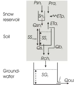
Several stores (e.g., soils, groundwater) and fluxes control hydrological drought development, as presented in the con-ceptual diagram in Fig. 1. This diagram is a simplified repre-sentation of reality. For instance, other stores than soil mois-ture and groundwater storage, such as bogs and lakes, are missing. Below-normal rainfall (Pra), often in combination with higher potential evapotranspiration (ETp), causes de-pletion of soil moisture storage (SS), which eventually leads to negligible recharge (Rch≈0) or lower than normal Rch from the soil to the groundwater system (SG) (e.g., Van La-nen et al., 2004a). In cold regions, drought can also occur due to either lower than normal temperatures (in particular longer below zero) or higher temperatures (periods above zero that normally are frost times), which is related to snow accumu-lation and melt (e.g., Van Loon et al., 2011; Staudinger et al., 2011; Van Loon and Van Lanen, 2012). In a drought sit-uation, usually there will be a below-normal recharge that feeds the groundwater system. River flow is then controlled by the groundwater storage (SG) (Fig. 1, non-shaded). Low groundwater storage at the start of the period with below-normal recharge, or a long-lasting period with below-below-normal
Fig. 1. Conceptual diagram of stores and fluxes controlling hy-drological drought development. Psn: precipitation as snow, Pra: precipitation as rain, Sn: snow storage, ETp: potential evapotran-spiration, ETa: actual evapotranevapotran-spiration, Qsn: snowmelt, SS: soil
water storage, SSmax: total available soil moisture, Qs: downward
flux across bottom of the soil (percolation), Qb: bypass flow, Rch:
groundwater recharge, SG: groundwater storage,j: groundwater
re-sponse parameter, and Qout: groundwater discharge.
recharge, will cause a drought in river flow to develop (hydro-logical drought). A hydro(hydro-logical drought will end when the recharge again returns to normal (or higher than normal) for a sufficient period of time. This can be triggered by rainfall or snowmelt.
The modeling framework introduced below combines a conceptual hydrological model (i.e., a soil water balance model, including a snow module) and a simple, spatially lumped groundwater model. This modeling framework sim-ulates stores and fluxes according to the diagram in Fig. 1.
2.1.1 Soil water balance model
A transient soil water balance model (shaded part of Fig. 1) that uses daily precipitation, temperature and reference evap-oration as forcing data was applied to simulate time series of daily snowmelt, snow accumulation, actual evapotranspi-ration, soil moisture storage and groundwater recharge (Van Lanen et al., 1996). The rather simple soil water model does not simulate capillary rise. The soil may consists of up to 10 different layers to model the unsaturated zone. Land use data and soil data were used to characterize the physical catch-ment structure. The model solves the following daily water balance equations:
SSt=SSt−1+Prat+Qsnt−ETat−Rcht (1)
where SS is soil water storage (mm), Pra rain-fall (mm day−1), Qsn snowmelt (mm day−1), ETa actual
evapotranspiration (mm day−1), Rch groundwater recharge
(mm day−1), Sn snow storage (mm), Psn snow fall (mm day−1), Qs downward flux from the soil water to the groundwater storage (mm day−1), Qb bypass flow (i.e., part of rainfall that bypasses the soil and enters the groundwater system (mm day−1)), andt time (day).
The model uses the snow accumulation and melt approach of the well-known hydrological model HBV, as described by Seibert (2005). Accumulation of precipitation as snow takes place if the temperature is lower than a threshold tempera-ture TT, which normally is close to 0◦C. Melting of snow (Qsnt) starts if the daily temperatureTt>TT, and is calcu-lated using a degree-day model; i.e., the daily temperature difference (Tt−TT) is multiplied by the parameter CFMAX (mm◦C−1day−1) to yield the daily amount of snowmelt. All
precipitation that falls as snow in the model is multiplied by a correction factor, SFCF, to account for snow losses (e.g., sublimation). The snowpack retains meltwater until the amount exceeds a certain threshold (CWH, defined as a frac-tion of the water equivalent of the snowpack). When the tem-peratureTt decreases below TT, water in the snowpack re-freezes, and this process is controlled by the parameter CFR and the temperature difference (TT−Tt).
Potential evapotranspiration (ETpt, mm day−1) was com-puted by multiplying the daily reference evaporation (ETot, mm day−1) according to Penman–Monteith (Allen et al., 1998) with time-dependent crop factors. Crops transpire at a potential rate as long as SSt is between soil moisture stor-age at field capacity (SSFC) and critical soil moisture
stor-age (SSCR), implying that ETat=ETpt. For drier conditions,
ETat becomes less than ETpt and is calculated by multi-plying ETpt with the factor (SSt−SSWP)/(SSCR−SSWP),
where SSWPis soil moisture storage at wilting point. ETat=
0 when the soil is drier than wilting point.
The downward flux from the soil to the groundwater (Qst) is simulated as
Qst =SSt−SSFC if SSt≥SSFC (3)
Qst =
SSt−SSCR
SSFC−SSCR
b
·kFC if SSCR<SSt<SSFC (4)
Qst =0 if SSt≤SSCR, (5)
wherekFCis unsaturated hydraulic conductivity at field
ca-pacity (mm day−1) andb(–) is a shape parameter that is
de-rived from the soil moisture retention and the unsaturated hy-draulic conductivity curves.
Equation (4), which uses a power function to simulate recharge for soils drier than field capacity, is similar to the response function of the HBV model (Seibert, 2005). Rain-fall bypassing the soil and directly feeding the groundwa-ter system (Qbt) may occur in dry clay-rich soils (e.g., Van
Stiphout et al., 1987; Bronswijk, 1988). This is accounted for by assuming that Qbt takes place if SSt<SSCR, and the
by-passing rainfall is set equal to a fixed fraction of the rainfall (Sect. 2.3.3):
Rcht=Qst+Qbt. (6)
2.1.2 Groundwater model
Simulated recharge (Eq. 6) is input to a lumped ground-water model (non-shaded part of Fig. 1) based upon linear reservoir theory. This model was applied to simulate time series of groundwater discharge into a stream (Van Lanen et al., 2004a). The groundwater model uses the De Zeeuw– Hellinga approach (Kraijenhof van de Leur, 1962; Ritzema, 1994):
Qoutt=Qoutt−1·exp
−1
j +Rcht·(1−exp
−1
j ), (7)
where Qout is groundwater discharge (mm day−1) andj is
a response parameter (day). The groundwater discharge is hereafter called discharge. For naturally drained aquifers, a general interpretation of the response parameter is (Birtles and Wilkinson, 1975)
j=µ·L
2
kD , (8)
where kD is transmissivity of the groundwater system (m2day−1),µstorage coefficient of the groundwater system (–), and L distance between streams (m). These three pa-rameters allow the calculation of the response parameter for a given groundwater system (e.g., quickly responding, slowly responding).
2.1.3 Drought identification
deficit volume, SDV). Droughts starting before the period to be analyzed or continuing after the end of the period were excluded. If a particular month has zero flow for more than 20 % of the years, Q80 for this month equals zero and no drought can be identified for this particular month. If for all 12 months Q80=0, then no drought can be identified at all. This happens regularly for grid cells in areas with ephemeral streams, i.e., areas with a hot arid climate or a very cold climate with permanent snow or ice. These grid cells were excluded from the analysis.
2.2 Similarity index
A similarity index (SI) was introduced as a quantitative mea-sure of agreement between drought characteristics obtained for different realizations. The SI was used to investigate the impact of climate, soils and groundwater systems on hy-drological drought. It is defined as the degree of overlap (100 % indicates complete overlap and 0 % no overlap) be-tween probability fields of two different climate, soil, and groundwater system realizations. Bivariate probability distri-butions were introduced not to perform extreme value anal-ysis as it is common in hydrological studies, but rather to investigate probability fields of drought duration and stan-dardized deficit volume (DD-SDV fields) as a mean to quan-tify agreement between two realizations. Parametric bivariate probability distributions regularly have been applied to study drought characteristics (e.g., Ashkar et al., 1998). However, these may not reveal significant relationships among drought characteristics under a wide range of environmental con-ditions as they are site-specific. Therefore, similar to Kim et al. (2003), non-parametric kernel density estimators (e.g., Wand, 1994; Wand and Jones, 1995) were adopted to deter-mine smoothed bivariate probability fields of drought char-acteristics, i.e., the joint probability density field of drought duration and standardized deficit volume. The approach of Wand and Jones (1995) was used to determine the level of smoothing. The 90 % probability field (90 % DD-SDV prob-ability field) rather than the whole density field was chosen to define SI for various combinations of climate, soil and groundwater system to ensure that the analysis was not too much affected by rare events.
A straightforward geometrical approach was adopted to determine the degree of overlap of the 90 % DD-SDV proba-bilities of two realizations. A rectangular field ofm· · ·n pix-els was defined, in which all possible 90 % DD-SDV prob-ability fields of climate, soil and groundwater system real-izations fit. The similarity index (SI) quantifies the degree of overlap (%) between two 90 % DD-SDV probability fields as follows:
SI=R1|R2
R1 ·100 (9)
R1= m
X
x=1
n
X
Y=1
MR1(m, n) if MR1(m, n)=1 (10)
Fig. 2.Cross table showing the number of possible SI cases when comparing three realizations R1, R2 and R3.
R1|R2= m
X
x=1
n
X
Y=1
MR1(m, n) if MR1(m, n)=1,
and MR2(m, n)=1 (11) where R1 is the 90 % DD-SDV probability field of climate, soil and groundwater system realization 1, and R1|R2 is the coinciding 90 % DD-SDV probability fields of climate, soil and groundwater system realizations 1 and 2. MR1 and MR2 are matrices: MR1 contains the conditional probabilities of climate, soil and groundwater system realization 1, and MR2 the field of climate, soil and groundwater system realization 2. MR1(m, n)and MR2(m, n)are binary quantities where 1 equals a value within, and 0 a value outside the 90 % DD-SDV probability field of realizations 1 and 2, respectively. In this studym·nwas set at 150·150.
A low SI implies that the 90 % DD-SDV probability field of the first realization substantially differs (in size and/or ori-entation) from the 90 % DD-SDV probability field of the sec-ond realization. This means that a significant number of DD-SDV combinations of realization 1 do not occur in realization 2. Hence the impact of climate and/or physical catchment structure of realization 1 on hydrological drought deviates from that presented by realization 2, which implies that the controls of the two realizations are different. On the contrary, a high SI represents a climate, soil, and groundwater system realization (realization 1) that has a high number of DD-SDV combinations that also occur in realization 2.
2.3 Data
2.3.1 Climatic data
Climatic data were derived from a global dataset, i.e., WATCH Forcing Data (WFD, Weedon et al., 2011), which has been made available through the EU-FP6 project WATCH (WATer and global CHange). This large-scale dataset consists of gridded time series of meteorological variables (e.g., rainfall, snowfall, temperature, wind speed) on a daily basis for the period 1958–2001. The data have a half-degree resolution and are available for 67 420 land grid cells. The WFD originate from modification (bias correc-tion) of the ECMWF ERA-40 reanalysis data (Uppala et al., 2005), which are daily data on a 1.125 degree spatial reso-lution. The ERA-40 data were interpolated to a half-degree global land grid (excluding Antarctica). Among others, the 2 m temperature and specific humidity were corrected for elevation differences between the 1.125◦ ERA-40 grid and the 0.5◦WFD grid. Average diurnal temperature range and average temperature were bias-corrected using Climatic Re-search Unit (CRU) data. Furthermore, the monthly number of “wet” days was bias-corrected using CRU data (Mitchell and Jones, 2005) and precipitation totals using GPCCv4 (Schneider et al., 2011).
In this study, WFD rainfall and snowfall data were added up to obtain daily total precipitation (Prat+ Psnt, Fig. 1). The hydrological model is based on the HBV approach (Sect. 2.1). Daily temperatureTt, which was retrieved from WFD, was used in combination with a predefined threshold temperature TT to determine whether precipitation falls as rainfall or snow. Daily minimum and maximum temperature were computed using the WFD 3-hourly temperature data. WFD (i.e., temperature, wind speed, altitude) were also used to compute daily reference evaporation (ETo) following the Penman–Monteith equation (e.g., Allen et al., 1998). Radia-tion from the WFD was not used because of inconsistencies in the daily meteorological data that are relevant for the com-putation of ETo (Melsen et al., 2011). Hence, net radiation used to compute ETo was derived from the WFD daily min-imum and maxmin-imum temperatures. The latitude was used to compute extraterrestrial radiation (Allen et al., 1998).
Parameters to model snow accumulation and melt (Sect. 2.1) were set following the recommendations by Seib-ert (2000, 2005) and Masih et al. (2010), who provide stan-dard parameter values and their range. Here, the threshold temperature TT was set at 0◦C and the degree-day parameter
CFMAX was assumed equal to 3.5 mm◦C−1day−1, which
reflects open landscape conditions. Snow losses (e.g., sub-limation) were assumed to be 20 %, i.e., SFCF=0.8, and the meltwater holding capacity (CWH) and the refreezing coefficient (CFR) were set at 0.1 and 0.05, respectively.
2.3.2 Selection of grid cells using the K¨oppen–Geiger
climatic map
The hydrological model was run for a high number of ran-domly selected land grid cells, representing the five K¨oppen– Geiger major climate types (Kottek et al., 2006; Peel et al., 2007). Prior to the selection of the grid cells, the K¨oppen– Geiger map was recomputed using the 44 yr of WFD climate data. The map of Kottek et al. (2006) could not be used since the WFD used other data sources and procedures (Weedon et al., 2011). The recomputation led to a change of subcli-mates in about 9 % of the grid cells of the revised K¨oppen– Geiger map. The area with arid climates slightly increased at the account of snow, and warm and temperate climates (Wanders et al., 2010).
The minimum number of grid cells (i.e., sample size) re-quired to determine if two 90 % DD-SDV probability fields (Sect. 2.2) significantly deviate was assessed using bootstrap-ping for each major climate type, soil and groundwater sys-tem realization. This method for assigning a level of relia-bility to the sample estimate was adopted because the theo-retical bivariate distribution function of drought duration and standardized deficit volume for the different realizations is unknown. The similarity index (SI), i.e., the degree of over-lap between the areas of the two 90 % DD-SDV probability fields, was also used as a measure for this purpose. Our ap-proach implied a step by step increase of the sample size by adding grid cells. If the SI of a particular sample size and the previous size approaches 100 %, then the sample size is assumed to be large enough. Each time one grid cell from the same climate, soil and groundwater system realization was added, the 90 % DD-SDV probability field was com-puted. Next, the SI between the current and previous sample was determined (Eq. 9). These sampling steps were carried out 39 times (last sample contained all drought events from 40 grid cells). This was repeated 40 times for the same cli-mate, soil and groundwater system realization, but retrieving different grid cells. Finally, the 5 % quantile (5 % lowest SI) was derived for each of the 39 sampling steps from the 40 se-ries of SI. If the 5 % quantile of SI among two subsequent samples was higher than 97.5 %, it was assumed that sample size is sufficiently large to conclude that the difference be-tween the samples is not significant (i.e., they come from the same population). In this way the minimum number of grid cells was estimated for each climate, soil and groundwater system realization (in total 45).
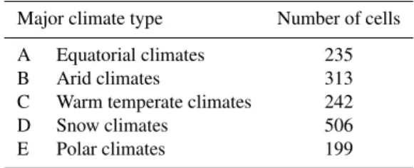
Table 1.Distribution of the selected grid cells over the K¨oppen– Geiger climate types.
Major climate type Number of cells
A Equatorial climates 235
B Arid climates 313
C Warm temperate climates 242
D Snow climates 506
E Polar climates 199
Table 1 gives the number of selected grid cells per major cli-mate type. The highest number of grid cells (34 %) was se-lected for the snow climate (D-climate). The other major cli-mate types (A, B, C and E) were represented by 16 %, 21 %, 16 % and 13 % of the grid cells, respectively. These numbers are well above the minimum number as specified through the bootstrapping. When comparing 90 % DD-SDV probability fields of two different climate, soil and groundwater system realizations, this number of cells ensures that a SI lower than 97.5 % is not caused by the sample size, but by differences in either the climate, soil or groundwater system (hereafter called significant difference).
2.3.3 Physical catchment structure
In total, nine realizations for the physical catchment structure were distinguished consisting of three mineral soils and three groundwater systems. Land use was assumed to be identical for all realizations, i.e., permanent grassland with a rooting depth of 50 cm. The soil information was derived from a stan-dard series of existing soils that predominantly differ in soil texture (W¨osten et al., 2001a, b). Each heterogeneous soil was assumed to consist of a 30 cm topsoil overlying a 20 cm thick subsoil with different soil moisture retention character-istics. The moisture retention data were used to select repre-sentative soils with a medium soil moisture supply capacity (light silty loam soil, hereafter Soil II) and soils with low and high supply capacity, i.e., a coarse sandy soil (Soil I) and a sandy loamy soil (Soil III), respectively (Table 2). To-tal available soil moisture (SSmax=SSFC−SSWP) is 31.9,
125.4 and 154.8 mm for Soils I, II and III, respectively, and readily available soil moisture (SSFC−SSCR) is 28.4, 73.7
and 94.5 mm. Soil II deviates about+10 % from the aver-age total and readily available soil moisture computed for the standard series of 15 mineral soils. For Soils I and III the deviation is about−65 and+40 %, respectively. Clearly the loamy soils (II and III) are more similar than the coarse sandy soil (Soil I) because of the skewed distribution of the soil moisture supply capacity over the soil textures. Mineral soils were only considered because peat soils cover only a small area on the globe. Rainfall (>2 mm day−1) bypassing the dry soil and directly feeding into the groundwater sys-tem (Eq. 6) was assumed to be equal to 50 % of the rainfall
and to occur when the soil is dryer than critical soil moisture storage (SSCR).
Three representative groundwater systems were defined through the response parameter j (Eq. 8). Values of j of 20 or 30 day are generally applicable to artificially drained fields and values of up to 2000 day to discharge from well-developed aquifers into streams (Peters, 2003). Com-prehensive drainage studies are the basis for Eqs. (7) and (8) and associatedj values (Kraijenhof van de Leur, 1962; Ritzema, 1994). Here j=250 day was selected to rep-resent an intermediately responding groundwater system. This, for example, holds for a catchment with a trans-missivity of 1000 m2d−1, a storage coefficient of 0.1 and a stream distance of about 1.5 km. Quickly and slowly sponding groundwater systems were defined through a re-sponse parameter of 100 and 1000 day, respectively, which still represent fairly common groundwater systems.
In summary, the proposed modeling framework was ap-plied to nine realizations of physical catchment structure for each of the 1495 grid cells, representing a fair coverage of the different climates across the world and, thus, a realistic range of drought characteristics. The introduced framework pro-vides a unique opportunity to explore the relative role of ma-jor climates, soils and groundwater systems on hydrological drought across the globe.
3 Results
3.1 Importance of climate
Table 2.Soil moisture characteristics of the three selected soils.
Soil Soil moisture content (vol. %) Soil moisture supply
Number Texture Topsoil Subsoil capacity (mm)
FC CR WP FC CR WP SSFC SSCR SSWP
I coarse 9.4 2.0 1.1 4.2 1.1 0.7 36.6 8.2 4.7
sand
II light silty 31.5 19.0 9.5 37.2 19.1 7.5 168.9 95.2 43.5
loam
III sandy 35.3 16.8 5.7 36.2 16.7 3.2 178.3 83.8 23.5
loam
(a)
Climate type
Number of droughts
A B C D E
0
20
40
60
80
100
120
● ● ● ● ●
● ● ● ● ● ●
● ● ● ●
● ●
● ● ● ●●
● ● ●
(b)
Climate type
Dur
ation (da
ys)
A B C D E
1
10
100
1000 ●
● ● ● ● ●
● ● ●
● ● ● ● ●
● ● ● ● ●
● ● ● ●
(c)
Climate type
Standardiz
ed Deficit V
olume
(d
a
y
−
1)
A B C D E
1e−04
0.01
0.1
1
10
100 ● ● ● ● ●
● ● ● ● ●
● ● ● ● ●
● ● ● ● ●
● ● ● ● ●
Fig. 3.Summary statistics (box: 25, 50 and 75 deciles, whiskers: 5 and 95 deciles) of hydrological drought characteristics of all drought
events for each of the major climate types (A–E); Soil II and groundwater systemj=250 day, period 1958–2001.(a)number of droughts,
(b)drought duration, and(c)standardized deficit volume. The circles represent extreme events beyond D95 for the 96, 97, 98, 99 and 100
deciles. Please note that y-axis of(a)is on linear scale, and(b)and(c)are on log scale.
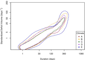
discharge, respectively). The snow climate (D-climate) takes an intermediate position (33 times the mean daily discharge). The 90 % DD-SDV probability field based on drought events of each K¨oppen–Geiger major climate type is shown in Fig. 4 for the reference situation. The 90 % DD-SDV prob-ability fields share a vast common area (implying a high SI), which would suggest a rather limited influence of climate on hydrological drought characteristics. However, there are also clear differences. The areas of the 90 % DD-SDV probability fields of the temperate and equatorial climates (types A and C) are significantly smaller than those of the arid and polar climates (types B and E), which is consistent with the conclu-sion of the summary statistics (Fig. 3). The area of the snow climate (type D) again takes an intermediate position.
The similarity index (SI), used to quantify the degree of similarity between the 90 % DD-SDV probability fields of two realizations, is calculated for the different climate types, as shown in Table 3. The SI for all major climates, except E-climates, is at least 65 % and usually over 75 % (only row-wise reading), which demonstrates a rather high simi-larity among most major climate types. The relatively small 90 % DD-SDV probability field of the temperate climate (Fig. 4, type C) largely coincides with the 90 % DD-SDV
Table 3.Similarity index (SIa) (%) for the K¨oppen–Geiger major climate types for catchments with a medium soil water supply ca-pacity (Soil II) and intermediately responding groundwater system
(j=250 d).
Major Major climate typeY
climate A B C D E
typeX
A 100 99b 90 93 100
B 70b 100 65 82 95
C 96 100 100 96 99
D 79 98 75 100 99
E 54 73 50 64 100
aSI<97.5 % implies that the difference is caused by
climate and cannot solely be explained by the sample size. SI = 100 % means that the drought durations and the standardized deficit volumes of two climates completely overlap; i.e., the two climates have the same effect on these
drought characteristics (Sect. 2.3).bRows give the degree
of overlap of climate typeXwithY, i.e., SI(X|Y); for
example, SI(A|B)=99means that A overlaps 99 % with B,
and SI(B|A)=70means that B overlaps 70 % with A (thus
the area of B>A; see Fig. 4).
3.2 Importance of soils and groundwater systems
The impact of climate on drought characteristics was dis-cussed in the previous section for a reference physical catch-ment structure, i.e., with a soil having a medium soil moisture capacity (Soil II) and an intermediately responding ground-water system (j=250 day). In this section the effect of the physical catchment structure is analyzed. Summary statistics of drought characteristics of all selected grid cells for each of the nine soil and groundwater system realizations are given in Fig. 5, irrespective of climate type (i.e., all climates lumped). It shows that the number of droughts, duration and standard-ized deficit volume are hardly affected by the soil moisture supply capacity for the selected moderately thick soils cov-ered with permanent grassland (Table 2). On the contrary, the responsiveness of the groundwater system has a major impact on hydrological drought characteristics, in particular on the number of droughts (all deciles). The median num-ber of droughts (D50) for a quickly responding groundwa-ter system (j =100 day) is about three times higher than for a slowly responding system (j=1000 day) (upper row). The range (D75–D25) in the number of droughts is twice as high for the quickly responding system. Differences in median drought duration are rather small (many minor droughts), but the lower number of droughts for the slowly responding system results in a D75 duration that is about twice as long as for a quickly responding system (middle row). Similar to drought duration, differences in standardized deficit volume between groundwater systems are not clearly seen in the me-dian plotted on a log scale (lower row). However, larger dif-ferences can be seen for the higher deciles. The D75 stan-dardized deficit volume of the quickly responding systems
Duration (days)
S
ta
n
d
a
rd
ize
d
D
e
fi
ci
t
V
o
lu
m
e
(
d
a
ys
−
1)
1
5
25
50
100
250
1 30 120 360 1080
●
●
●
●
●
Climate A B C D E
Fig. 4.90 % bivariate probability fields of hydrological drought du-ration and standardized deficit volume for the five K¨oppen–Geiger major climate types (A–E) for the reference situation (i.e., a medium soil water supply capacity (Soil II) and intermediately responding
groundwater system (j=250 d)). We used the double square root
of the drought duration because of the wide spread of the durations (the kernel smoothing, Sect. 2.2, allows drought durations smaller than one day).
is about two and half times higher than that of the slowly responding system.
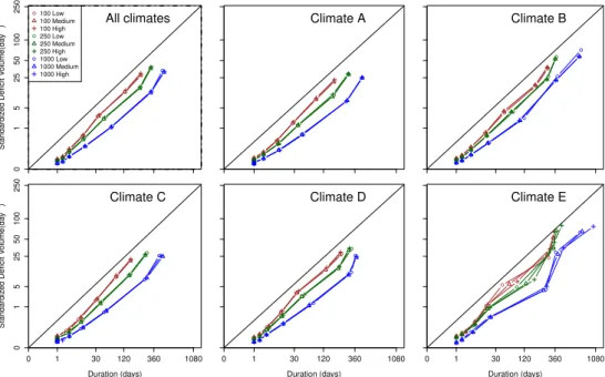
The relation between the drought duration and standard-ized deficit volume for all climates lumped is plotted for a number of deciles in Fig. 6. The small influence of the se-lected soils and the large impact of groundwater systems, in particular on the duration, are here confirmed. The lines for the three soils more or less coincide, whereas these clearly deviate for the three groundwater systems. The patterns seen for the five K¨oppen–Geiger climate types are more or less similar and almost identical to the lumped one (upper left). The patterns for the equatorial, temperate and snow climates (A-, C- and D-climates) are most similar to the lumped one. The patterns for the more extreme climates (arid and po-lar, B- and E-climates) deviate more, in particular for the groundwater systems with a quicker response (j =100 and 250 day).
j=100 days
Number of droughts
0 50 100 150 ● ● ● ● ● ●●●● ● ● ● ● ● ● j=250 days ● ● ● ● ● ● ● ● ● ● ● ● ● ● ● j=1000 days ● ● ● ● ● ● ● ● ● ● ●● ● ● ● Dur ation (da ys) 1 10 100 1000 ● ● ● ● ● ●●●●● ●●●●● ● ● ● ● ● ● ● ● ● ● ●● ● ● ● ● ● ● ● ● ● ● ● ● ● ● ● ● ● ● Soil type Standardiz
ed Deficit V
olume (d a y − 1)
I II III
1e−04 0.1 10 ● ● ● ● ● ●●●●● ●●●●● Soil type
I II III
● ● ● ● ● ●● ● ● ● ●● ● ● ● Soil type
I II III
● ● ● ● ● ●●● ● ● ● ● ● ● ●
Fig. 5.Summary statistics (box: 25, 50 and 75 deciles, whiskers: 5 and 95 deciles) of hydrological drought characteristics (number of droughts, drought duration, standardized deficit volume) of all drought events (1495 grid cells) for three soils and three different groundwater systems. The circles represent extreme events beyond D95 for the 96, 97, 98, 99 and 100 deciles. Please note that y-axis is on log scale.
●● ● ● ● ● ● Standardiz
ed Deficit V
olume(day − 1) 0 1 5 25 50 100 250 ●● ● ● ● ● ● ● ● ● ● ● ● ● All climates ● ● ● 100 Low 100 Medium 100 High 250 Low 250 Medium 250 High 1000 Low 1000 Medium 1000 High ● ● ● ● ● ● ● ● ● ● ● ● ● ● ● ● ● ● ● ● ● Climate A ●● ● ● ● ● ● ●● ● ● ● ● ● ●● ● ● ● ● ● Climate B ● ● ● ● ● ● ● Duration (days) Standardiz
ed Deficit V
olume(day
−
1)
0 1 30 120 360 1080
0 1 5 25 50 100 250 ● ● ● ● ● ● ● ● ● ● ● ● ● ● Climate C ●● ● ● ● ● ● Duration (days)
0 1 30 120 360 1080
●● ● ● ● ● ● ●● ● ● ● ● ● Climate D ●● ● ● ● ● ● Duration (days)
0 1 30 120 360 1080
●● ● ● ● ● ● ●● ● ● ● ● ● Climate E
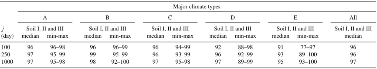
small (96–98 %). For the intermediately and slowly respond-ing groundwater systems (j =250 and 1000 day), the me-dian SI is at least 93 % and in most cases 96 % or higher, which shows that the 90 % DD-SDV probability fields of the various soils almost completely overlap, so that the in-fluence of the selected soils on hydrological drought charac-teristics is rather limited. The impact is somewhat higher for the quickly responding groundwater system (j=100 day), in particular for the polar climates (E-climate), i.e., median SI=91 %. Most of the SIs in Table 4 are high, meaning that the 90 % DD-SDV probability fields do not deviate much, al-though these small deviations are still significant (<97.5 %, Sect. 2.3).
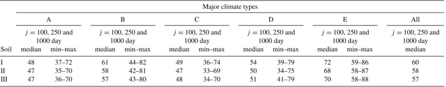
Similarly as for the soils, the influence of the responsive-ness of the groundwater system on the SI is determined (Ta-ble 5) for each of the three soils and five major climates sep-arately. In this case, the median SI is found out of the six possible combinations of three groundwater systems (Fig. 2) for a particular climate type and soil realization. The min-imum and maxmin-imum SI are also provided. All SIs are be-low 80 % (except maximum SI for the B- and E-climates), meaning that the 80 % DD-SDV probability fields of the var-ious groundwater systems deviate significantly. The lowest SI (33 %) is found when comparing the 90 % DD-SDV prob-ability fields of the quickly and slowly responding groundwa-ter systems (j =100 and 1000 day) for Soil II and climate C, whereas the maximum SI (88 %) is found for the fields of the quickly and intermediately responding groundwater systems (j=100 and 250 day) for Soil III and E-climate.
3.3 Sensitivity analysis
Additional sensitivity analyses for the reference situation (Soil II,j=250 day) demonstrated that the selected parame-terizations (i.e., land use and snow) of the conceptual hydro-logical model (Sect. 2.3) only had limited influence on the obtained SI (Sect. 3.1). In the land use sensitivity analysis, the permanent grassland was replaced by more taller perma-nent vegetation type having a 10 % higher potential evapo-transpiration (e.g., shrubs, trees). This also meant a larger rooting depth, which was increased from 0.50 m (Sect. 2.3) to 1.50 m. Although land use had impact on simulated dis-charge and the 90 % DD-SDV probability field, the SIs of the major climate types only showed a minor change compared to the reference situation (around 2 % for the A-, C- and D-climates, and around 6 % for the more extreme B- and E-climates, compared to Table 3). In the snow sensitivity anal-ysis, two additional snow parameter sets selected within the normal parameter range (Seibert, 2000, 2005; Seibert et al., 2000; Wid´en-Nilsson et al., 2007; Van der Knijff and De Roo, 2008; Masih et al., 2010) were defined to investigate the influence on SI. The first set resulted into earlier snow accu-mulation and later melt (TT=1.0◦C) and a slower snowmelt (CFMAX=2.0 mm◦C−1day−1). The second parameter set led to later accumulation and earlier melt (TT= −1.0◦C)
and faster snowmelt (CFMAX = 4.5 mm◦C−1day−1). The
analysis showed that the SIs of the major climate types changed only slightly compared to the reference situation in Table 3. For the scenario with less snow, the SIs did not devi-ate more than 1 %, whereas for the scenario with more snow the differences were somewhat larger (less than 1.5 % for the A-, B- and C-climates, and 2.4 and 4.1 % for the D- and E-climates).
4 Discussion
4.1 Climate control on hydrological drought
The B- and E-climates have lower number of droughts, longer drought durations and larger standard deficit volumes than the other major climates (Fig. 3), because of very irregu-lar rain (B type) or erratic snowmelt peaks that interrupt long snow accumulation periods (E type). This large interannual climate variability of the B- and E-climates (e.g., Stahl and Hisdal, 2004) gives rise to hydrographs with sustained pe-riods of low discharge on which irregular sharp flow peaks are superimposed. On the contrary, the regular rain in the A- and C-climates prevents the development of long-lasting droughts with large standardized deficit volumes implying rather small 90 % DD-SDV probability fields compared to those of the B- and E-climates (Fig. 4). These differences in the 90 % DD-SDV probability fields among the climates are reflected in the SI (Table 3), i.e., high SIs for the A- and C-climates and rather low for the B- and E-climates. The 90 % DD-SDV probability fields of the snow climates (D-climates) are larger than that of types A and C, resulting in lower SI (Table 3). In the A- and C-climates drought devel-opment is strongly restricted by the seasons, whereas in the D-climate summer drought can continue into winter result-ing in very long droughts (Van Loon and Van Lanen, 2012), which can be prolonged by delayed snowmelt. Drought in the D-climate always ends by a snowmelt peak feeding soil moisture, groundwater storage (SSt, SGt) and eventually dis-charge (Qoutt, Fig. 1). These consistent peaks do not exist in the B- and E-climates, which are more irregular and, hence, lead to longer drought than in the D-climate.
4.2 Catchment control on hydrological drought
Table 4.Impact of soils on the similarity index (SI) (%) for the five K¨oppen–Geiger major climate types and three groundwater systems.
Major climate types
A B C D E All
j Soil I. II and III Soil I, II and III Soil I, II and III Soil I, II and III Soil I, II and III Soil I, II and III
(day) median min-max median min-max median min-max median min-max median min-max median
100 96 96–98 96 96–99 96 94–99 92 88–98 91 77–97 96
250 97 95–99 99 95–99 96 93–99 96 92–99 93 89–100 96
1000 97 95–98 98 92–100 97 95–98 97 89–99 95 93–100 97
or heavy clay soils) that were not included in this study may generate a more irregular discharge (e.g., Bouma et al., 2011) and, hence, might exhibit a more prominent role of soils on hydrological drought characteristics.
Responsiveness of groundwater systems has a large effect on drought characteristics (Fig. 5). Flashy hydrographs, asso-ciated with quickly responding groundwater systems, cause a high number of drought events of short durations. Hydro-graphs representative of slowly responding groundwater sys-tems are rather smooth and do not show direct response to rainfall or snowmelt; i.e., the response is delayed and at-tenuated. Droughts in such hydrographs are rarer, but last longer. In our modeling experiment the median number of droughts for the quickly responding groundwater system is three times higher than that of the slowly responding sys-tem. These results are supported by earlier-documented site-specific drought studies (e.g., Tallaksen et al., 1997; Peters et al., 2003; Van Lanen et al., 2004a, b; Fleig et al., 2006; Van Lanen and Tallaksen, 2007, 2008; Van Loon and Van Lanen, 2012) and by studies on the modification of climate– river flow associations by basin characteristics (e.g., Tague et al., 2008; Laize and Hannah, 2010). The larger influ-ence of groundwater systems on hydrological drought char-acteristics compared to soils is also reflected in the sub-stantially lower SIs of groundwater systems (Table 5). The somewhat smaller influence of the groundwater system in the extreme climates (B- and E-climates) is likely a result of the generally low recharge in these climates leading to low SGt variation among the studied groundwater systems. Longer droughts, typical for slowly responding groundwa-ter systems, do not always coincide with larger standardized deficit volumes (Fig. 5). A smooth discharge hydrograph re-sults in smaller departures from the threshold (i.e., smaller deficits) compared to the more flashy hydrographs of the quickly responding groundwater systems. The net effect of longer durations but smaller departures from the threshold of the slowly responding groundwater systems leads to slightly lower standardized deficit volumes than those that can be found for the quickly responding systems. Whether the more long-lasting drought with less deficit or the short-lived with higher deficit has the more severe impacts depends on the affected sector (e.g., aquatic ecology or water supply). The simulated time series with the conceptual hydrological model provide potential to unravel effects of climate control versus
physical catchment structure on reported trends in hydrolog-ical drought (e.g., Stahl et al., 2010, 2012; Hannaford et al., 2013). The model outcome can also be used to support stud-ies on drought propagation (i.e., the conversion of a meteoro-logical drought into a hydrometeoro-logical drought; e.g., Changnon, 1987; Peters et al., 2003; Tallaksen et al., 2009; Van Loon and Van Lanen, 2012), which also depends on climate and physical catchment structure.
4.3 Modeling framework
Table 5.Impact of groundwater systems on the similarity index (SI) (%) for five K¨oppen–Geiger major climate types and three soils.
Major climate types
A B C D E All
j=100, 250 and j=100, 250 and j=100, 250 and j=100, 250 and j=100, 250 and j=100, 250 and
1000 day 1000 day 1000 day 1000 day 1000 day 1000 day
Soil median min–max median min–max median min–max median min–max median min–max median
I 48 37–72 61 44–82 49 36–74 54 39–79 72 59–86 60
II 47 35–70 58 42–81 47 33–69 50 34–75 68 58–87 58
III 47 36–70 57 43–80 48 34–70 51 41–79 70 58–88 57
studies demonstrate common problems in reliably simulat-ing low streamflow and steep recessions (e.g., Pushpalatha et al., 2011; Staudinger et al., 2011), but indicate that reliabil-ity of model results is satisfactory for drought analysis based on the threshold level approach. Furthermore, the WATCH Forcing Data (Sect. 3.2), which were used as input, agree rather well with independent data, e.g., FLUXNET (Weedon et al., 2011), although drought characteristics for the arid and polar climates (B- and E-climates) realizations would proba-bly have been more robust if longer time series could have been used. The nine soil and groundwater system realiza-tions cover a wide range of physical catchment structures across the world. The SIs for realizations with the quickly re-sponding groundwater system, which generates more flashy hydrographs, illustrate that even under these conditions the responsiveness of the groundwater system is important rela-tive to climate. Sensitivity analyses showed that the impact of land use (implicitly also soil) and parameterization of snow accumulation and melt (Sect. 3.3) on the SI of climate, soil and groundwater system realizations is limited, implying that the outcome of our study is rather robust.
4.4 Importance of groundwater
The groundwater system was demonstrated to be as impor-tant as climate control for the development of hydrological drought, and selected soils under grassland seem to be of less importance. A proper assessment of hydrological drought re-quires adequate simulation of groundwater responsiveness. Most hydrological models that operate at the river basin scale have the potential to sufficiently model the groundwater sys-tem for drought studies (e.g., Van Lanen et al., 2004b; Tal-laksen et al., 2009; Van Loon et al., 2011). However, recent low flow and hydrological drought studies at the continental scale that analyze the outcome of large-scale models (e.g., Stahl et al., 2011; Prudhomme et al., 2011; Gudmundsson et al., 2012) reveal that these models tend to over- or un-derestimate river flow variability and perform less well for the lower flows. This suggests that storage processes (e.g., Van Loon et al., 2012), in particular the groundwater system, might not be well described yet. This lack of groundwater representation in large-scale models could also be the reason that a set of eight large-scale models produces a large spread
in predicted trends in monthly river flow over the second part of the last century (Stahl et al., 2012). The importance of groundwater for large-scale studies is also of significance through its influence on soil moisture and evapotranspiration, as reported by several authors (e.g., Bierkens and Van den Hurk, 2007; Anyah et al., 2008; Goderniaux et al., 2009; Fan and Miguez-Macho, 2010). However, progress has been re-stricted because the current generation of large-scale models has grid cells with a resolution of 25–50 km. The potential to improve the representation of the groundwater system in large-scale models will largely increase when future models are able to reach spatial resolutions down to 1 km, as sug-gested by Wood et al. (2010). At this scale, variation in more local hydrogeological conditions and lateral flow can be in-cluded, although model parameterization will remain a chal-lenge (e.g., Sutanudjaja et al., 2011).
5 Conclusions
The impact of climate and physical catchment structure on hydrological drought characteristics has been investigated through a controlled modeling experiment that identified drought in simulated daily discharge in a representative num-ber of grid cells across the world over the second part of the 20th century. This has been done for nine soil and groundwa-ter system realizations. The drought analysis approach that was adopted identified drought in discharge as an anomaly from a site-specific, monthly variable threshold, which im-plies that drought occurs everywhere under all environmen-tal conditions. Summary statistics and a similarity index (SI) were used to investigate the relative importance of climate, soil and groundwater systems. The SI is a comprehensive measure that compares the overlap of the 90 % bivariate probability density fields of drought duration and standard-ized deficit volume (90 % DD-SDV probability field) of two climate, soil and groundwater system realizations. It provides the level of agreement of two realizations with respect to drought characteristics (high SI implies highly comparable impact of two realizations on hydrological drought charac-teristics, and low SI the opposite).
a large number of drought events have similar combinations of duration and standardized deficit volume, irrespective of climate type. 90 % DD-SDV probability fields of the equato-rial climate (type A) and the temperate climate (type C) have most in common, mutually, and with the other three major climates, which give rise to rather high SIs. Some droughts of the snow climate (type D) last longer and build up a larger deficit than those of the A- and C-climates. Part of the hydro-logical characteristics of drought events in the arid and polar climates (types B and E) clearly deviate from the three other climates due to larger interannual climate variability.
The selected moderately thick soils under grassland in this study were found to have little effect on drought characteris-tics, in contrast to groundwater systems. SIs of realizations where only soils have been varied confirm these findings. Median SIs for the soils are higher than 90 %, irrespective of climate, and usually above 95 %, meaning that the 90 % DD-SDV probability fields barely differ. The responsiveness of groundwater systems to groundwater recharge has strong control on the development of hydrological drought. Slowly responding groundwater systems have clearly fewer drought events than quickly responding systems, but they last longer. The major impact of groundwater systems on the develop-ment of hydrological drought is also illustrated by the median SIs that are lower than 60 % for almost all climate conditions. In many realizations, SIs for groundwater systems are lower than, or as low as, the lowest SI for all climate types.
The groundwater system was demonstrated to be as im-portant as climate control for the development of hydrolog-ical drought. A proper assessment of hydrologhydrolog-ical drought includes more than an evaluation of meteorological drought (e.g., through the standard precipitation index). This assess-ment is essential for appropriate water resources manage-ment and planning, meaning that models that are used for drought forecasting and prediction should adequately sim-ulate groundwater responsiveness. Most river basin models have the potential to sufficiently model the groundwater sys-tem for drought studies, but the subsurface module (ground-water part) of large-scale models needs improvement. A bet-ter representation of the subsurface in large-scale models would help to better understand historic global and continen-tal drought and, hence, to better predict large-scale drought in response to global change.
Acknowledgements. This research was undertaken as part of the European Union (FP6) funded Integrated Project Water and Global Change (WATCH, contract 036946) and contributes to EU FP7 Collaborative project DROUGHT-R&SPI (grant 282769). One of the authors is supported by NWO (NWO GO-AO/30). The authors thank Paul Torfs (Wageningen University) for his support with writing up the mathematical equations. The research is part of the programme of the Wageningen Institute for Environment and Climate Research (WIMEK-SENSE), and it supports the work of the UNESCO-IHP VII FRIEND programme.
Edited by: F. Pappenberger
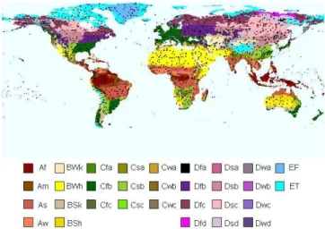
Appendix A
Fig. A1.Global map of K¨oppen–Geiger climate types derived from the WATCH Forcing Data set over the period 1958–2001 by Wanders et al. (2010). Black dots indicate a total of 1495 locations used in this study.
References
Allen, R. G., Pereira, L. S., Raes, D., and Smith, M.: Crop Evap-otranspiration: Guidelines for Computing Crop Water Require-ments, FAO Irrig. Drain. paper 56, Rome, 1988.
Anyah, R. O., Weaver, C. P., Miguez-Macho, G, Fan, Y., and Robock, A.: Incorporating water table dynamics in climate modeling: 3. simulated groundwater influence on coupled land-atmosphere variability, J. Geophys. Res., 113, D07103, doi:10.1029/2007JD009087, 2008.
Andreadis, K., Clark, E., Wood, A., Hamlet, A., and Letten-maier, D.: Twentieth-century drought in the conterminous United States, J. Hydrometeorol., 6, 985–1001, 2005.
Ashkar, F., Jabi, N. E. I., and Issa, M.: A bivariate analysis of the volume and duration of low-flow events, Stoch. Hydrol. Hy-draul., 12, 97–116, 1998.
Bates, B., Kundzewicz, Z., Wu, S., and Palutikof, J.: Climate Change and Water. Technical Paper of the Intergovernmental Panel on Climate Change, Intergovernmental Panel on Climate Change, Geneva, 2008.
Beven, K.: Towards integrated environmental models of every-where: uncertainty, data and modelling as a learning process, Hydrol. Earth Syst. Sci., 11, 460–467, doi:10.5194/hess-11-460-2007, 2007.
Bergstr¨om, S.: Development and application of a conceptual runoff model for Scandinavian catchments, SMHI RHO 7, 134 pp., Norrk¨oping, 1976.
Bierkens, M. F. P. and Van den Hurk, B. J. J. M.: Ground-water convergence as a possible mechanism for multi-year persistence in rainfall, Geophys. Res. Lett., 34, L02402, doi:10.1029/2006GL028396, 2007.
regulation, Water Resour. Res., 11, 571–580, 1975.
Bouma, J., Droogers, P., Sonneveld, M. P. W., Ritzema, C. J., Hunink, J. E., Immerzeel, W. W., and Kauffman, S.: Hydropedo-logical insights when considering catchment classification, Hy-drol. Earth Syst. Sci., 15, 1909–1919, doi:10.5194/hess-15-1909-2011, 2011.
Bronswijk, J. J. B.: Modelling of water balance, cracking and sub-sidence of clay soils, J. Hydrol., 97, 199–212, 1988.
Casado S´aenz, M., Montoya, F. F., and Gil de Mingo, R.: The role of groundwater during drought, in coping with drought risk in agri-culture and water supply systems, edited by: Iglesias, A., Gar-rote, L., Cancelliere, A., Cubillo, F., and Wilhite, D. A., Springer, Adv. Nat. Technol. Haz., 26, 221–241, doi:10.1007/978-1-4020-9045-5, 2009.
Changnon Jr., S. A.: Detecting Drought Conditions in Illinois, Illi-nois State Water Survey Champaign, Circular 169, 1987. Corzo Perez, G. A., van Huijgevoort, M. H. J., Voß, F., and van
La-nen, H. A. J.: On the spatio-temporal analysis of hydrological droughts from global hydrological models, Hydrol. Earth Syst. Sci., 15, 2963–2978, doi:10.5194/hess-15-2963-2011, 2011. Dai, A.: Drought under global warming: a review, advanced review,
Clim. Change, 2, 45–65, doi:10.1002/wcc.81, 2011.
Dai, A.: Increasing drought under global warming in
ob-servations and models, Nat. Clim. Change, 3, 52–58,
doi:10.1038/nclimate1633, 2013.
D¨oll, P., Kaspar, F., and Lehner, B.: A global hydrological model for deriving water availability indicators: model tuning and vali-dation, J. Hydrol., 270, 105–134, 2003.
EEA: Mapping the impacts of natural hazards and technological ac-cidents in Europe. An overview of the last decade, EEA Techni-cal report No 13/2010, Copenhagen, 2010.
Engeland, K. and Hisdal H.: A comparison of low flow estimates in ungauged catchments using regional regression and the HBV-model, Int. Ser. Prog. Wat. Res., 23, 2567–2586, 2009.
Falkenmark, M., Rockstr¨om, J., and Karlberg L.: Present and future water requirements for feeding humanity, Food Sec., 1, 59–69, 2009.
Fan, Y. and Miguez-Macho, G.: Potential groundwater contribu-tion to Amazon evapotranspiracontribu-tion, Hydrol. Earth Syst. Sci., 14, 2039–2056, doi:10.5194/hess-14-2039-2010, 2010.
Fleig, A. K., Tallaksen, L. M., Hisdal, H., and Demuth, S.: A global evaluation of streamflow drought characteristics, Hydrol. Earth Syst. Sci., 10, 535–552, doi:10.5194/hess-10-535-2006, 2006. Gerten, D., Heinke, J., Hoff, H., Biemans, H., Fader, M.,
and Waha, K.: Global water availability and requirements for future food production, J. Hydrometeorol., 12, 885–899, doi:10.1175/2011JHM1328.1, 2011.
Goderniaux, P., Brouy`ere, S., Fowler, H. J., Blenkinsop, S., Ther-rien, R., Orban, P., and Dassargues, A.: Large scale surface – subsurface hydrological model to assess climate change impacts on groundwater reserves, J. Hydrol., 373, 122–138, doi:10.1016/j.jhydrol.2009.04.017, 2009.
Gudmundsson, L., Tallaksen, L. M., Stahl, K., and Fleig, A. K.: Low-frequency variability of European runoff, Hydrol. Earth Syst. Sci., 15, 2853–2869, doi:10.5194/hess-15-2853-2011, 2011.
Gudmundsson, L., Tallaksen, L. M., Stahl, S., Clark, D., Hage-mann, S., Bertrand, N., Gerten, D., Hanasaki, N., Heinke, J., Voß, F., and Koirala, S.: Comparing large-scale hydrological
models to observed runoff percentiles in Europe, J. Hydrome-teorol., 13, 604–620, doi:10.1175/JHM-D-11-083.1, 2012. Haddeland, I., Clark, D., Franssen, W., Ludwig, F., Voss, F.,
Arnell, N., Bertrand, N., Best, M., Folwell, S., Gerten, D., Gomes, S., Gosling, S. N., Hagemann, S., Hanasaki, N., Hard-ing, R., Heinke, J., Kabat, P., Koirala, S., Oki, T., Polcher, J., Stacke, T., Viterbo, P., Weedon, G. P., and Yeh, P.: Multi-model estimate of the global water balance: setup and first results, J. Hy-drometeorol., 12, 869–884, doi:10.1175/2011JHM1324.1, 2011. Hannaford, J., Lloyd-Hughes, B., Keef, C., Parry, S., and Prud-homme, C.: Examining the large-scale spatial coherence of Eu-ropean drought using regional indicators of precipitation and streamflow deficit, Hydrol. Process., 25, 1146–1162, 2010. Hannaford, J., Buys, G., Stahl, K., and Tallaksen, L. M.: The
in-fluence of decadal-scale variability on trends in long European streamflow records, Hydrol. Earth Syst. Sci. Discuss., 10, 1859– 1896, doi:10.5194/hessd-10-1859-2013, 2013.
Hannah, D. M., Demuth, S., Van Lanen, H. A. J., Looser, U., Prud-homme, C., Rees, R., Stahl, K., and Tallaksen, L. M.: Large-scale river flow archives: importance, current status and future needs, Hydrol. Process., 25, 1191–1200, 2010.
Hisdal, H., Stahl, K., Tallaksen, L. M., and Demuth, S.: Have streamflow droughts in Europe become more severe or frequent?, Int. J. Climatol., 21, 317–333, 2001.
Hisdal, H., Tallaksen, L. M., Clausen, B., Peters, E., and Gus-tard, A.: Hydrological drought characteristics, in: Hydrological drought processes and estimation methods for streamflow and groundwater, edited by: Tallaksen, L. M. and Van Lanen, H. A. J., Dev. Water Sci., 48, 139–198, 2004.
ISDR: Global assessment report on disaster risk reduction. risk and poverty in a changing climate – invest today for a safer tomorrow, United Nations, Geneva, 2009.
Kim, T.-W., Valde’s, J. B., and Yoo, C.: Nonparametric approach for estimating return periods of droughts in arid regions, J. Hydrol. Eng., 8, 237–246, 2003.
Kottek, M., Grieser, J., Beck, C., Rudolf, B., and Rubel, F.: World Map of the K¨oppen–Geiger climate classification updated, Mete-orol. Z., 15, 259–263, doi:10.1127/0941-2948/2006/0130, 2006. Kraijenhof van de Leur, D. A.: Some effects of the unsaturated zone on nonsteady free-surface groundwater flow as studied in a sealed granular model, J. Geophys. Res., 67, 4347–4362, 1962. Laiz´e, C. R. L. and Hannah, D. M.: Modification of climate-river flow associations by basin properties, J. Hydrol., 389, 186–204, 2010.
Leblanc, M. J., Tregoning, P., Ramillien, G., Tweed, S. O., and Fakes, A.: Basin-scale, integrated observations of the early 21st century multiyear drought in southeast Australia, Water Resour. Res., 45, W04408, doi:10.1029/2008WR007333, 2009. Lewis, S. L., Brando, P. M., Phillips, O. L., Van der
Heij-den, G. M. F., and Nepstad, D.: The 2010 Amazon Drought, Sci-ence, 331, p. 554, 2011.
Masih, I., Uhlenbrook, S., Maskey, S., and Ahmad, M. D.: Region-alization of a conceptual rainfall-runoff model based on similar-ity of the flow duration curve: a case study from the semi-arid Karkheh basin, Iran, J. Hydrol. 391, 188–201, 2010.
Forcing Data, WATCH Technical Report No. 39, available at: www.eu-watch.org/publications/technical-reports (last access: 1 September 2012), 2011.
Mishra, K. K. and Singh, V. P.: A review of drought concepts, J. Hydrol., 391, 202–216, 2010.
Mitchell, T. D. and Jones, P. D.: An improved method of construct-ing a database of monthly climate observations and associated high-resolution grids, Int. J. Climatol., 25, 693–712, 2005. Peel, M. C., McMahon, T. A., and Pegram, G. S.: Global analysis
of runs of annual precipitation and runoff equal to or below the median: run magnitude and severity, Int. J. Climatol., 25, 549– 568, 2005.
Peel, M. C., Finlayson, B. L., and McMahon, T. A.: Updated world map of the K¨oppen–Geiger climate classification, Hy-drol. Earth Syst. Sci., 11, 1633–1644, doi:10.5194/hess-11-1633-2007, 2007.
Peters, E.: Propagation of drought through groundwater systems. Il-lustrated in the Pang (UK) and Upper-Guadiana (ES) catchments, PhD thesis, Wageningen University, The Netherlands, 2003. Peters, E., Torfs, P. J. J. F., Van Lanen, H. A. J., and Bier, G.:
Prop-agation of drought through groundwater – a new approach using linear reservoir theory, Hydrol. Process., 17 3023–3040, 2003. Peters, E., Bier, G., Van Lanen, H. A. J., and Torfs, P. J. J. F.:
Propa-gation and spatial distribution of drought in a groundwater catch-ment, J. Hydrol., 321, 257–275, 2006.
Prudhomme, C., Parry, S., Hannaford, J., Clark, D. B., Hage-mann, S., and Voss, F.: How well do large-scale models repro-duce regional hydrological extremes in Europe?, J. Hydrometeo-rol., 12, 1181–1204, doi:10.1175/2011JHM1387.1, 2011. Pushpalatha, R., Perrin, C., Moine, N. L., Mathevet, T., and
Andr´eassian, V.: A downward structural sensitivity analysis of hydrological models to improve low-flow simulation, J. Hydrol., 411, 66–76, doi:10.1016/j.jhydrol.2011.09.034, 2011.
Ritzema, H. P. (Ed.): Subsurface flow to drains, In: Drainage Princi-ples and Applications, 2nd Edn., International Institute for Land Reclamation and Improvement, Wageningen, 263–303, 1994. Schneider, U., Becker, A., Meyer-Christoffer, A., Ziese, M.,
and Rudolf, B.: Global Precipitation Analysis Products of the GPCC. Global Precipitation Climatology Centre (GPCC), Deutscher Wetterdienst, Offenbach a. M., Germany, avail-able at: ftp://ftp-anon.dwd.de/pub/data/gpcc/PDF/GPCC intro products 2008.pdf (last access: 24 October 2012), 2011. Seibert, J.: Multi-criteria calibration of a conceptual runoff model
using a genetic algorithm, Hydrol. Earth Syst. Sci., 4, 215–224, doi:10.5194/hess-4-215-2000, 2000.
Seibert, J.: HBV light version 2, user’s manual, available at: http:
//people.su.se/∼jseib/HBV/HBV manual 2005.pdf (last access:
25 October 2012), 2005.
Seibert, J., Uhlenbrook, S., Leibundgut, C., and Halldin, S.: Mul-tiscale calibration and validation of a conceptual rainfall-runoff model, Phys. Chem. Earth B, 25, 59–64, 2000.
Seneviratne, S. I., Nicholls, N., Easterling, D., Goodess, C. M., Kanae, S., Kossin, J., Luo, Y., Marengo, J., McInnes, K., Rahimi, M., Reichstein, M., Sorteberg, A., Vera, C., and Zhang, X.: Changes in climate extremes and their impacts on the natural physical environment, in: Managing the Risks of Extreme Events and Disasters to Advance Climate Change Adaptation, edited by: Field, C. B., Barros, V., Stocker, T. F., Qin, D., Dokken, D. J., Ebi, K. L., Mastrandrea, M. D., Mach, K. J., Plattner, G.-K.,
Allen, S. K., Tignor, M., and Midgley, P. M., A Special Report of Working Groups I and II of the Intergovernmental Panel on Cli-mate Change (IPCC), Cambridge University Press, Cambridge, UK, and New York, NY, USA, 109–230, 2012.
Sheffield, J. and Wood, E. F.: Global trends and variability in soil moisture and drought characteristics, 1950–2000, from observation-driven simulations of the terrestrial hydrologic cy-cle, J. Climate, 21, 432–458, 2008a.
Sheffield, J. and Wood, E. F.: Projected changes in drought oc-currence under future global warming from model, multi-scenario, IPCC AR4 simulations, Clim. Dynam., 31, 79–105, 2008b.
Sheffield, J., Andreadis, K., Wood, E. F., and Lettenmaier, D.: Global and continental drought in the second half of the twentieth century: severity-area-duration analysis and temporal variability of large-scale events, J. Climate, 22, 1962–1981, 2009.
Sheffield, J., Wood, E. F., and Roderick, M. L.: Little change in global drought over the past 60 years. Nature, 491, 435-438, doi:10.1038/nature11575, 2012.
Shukla, S. and Wood, A.: Use of a standardized runoff index for characterizing hydrologic drought, Geophys. Res. Lett., 35, L02405, doi:10.1029/2007GL032487, 2008.
Smakhtin, V. U.: Low flow hydrology: a review, J. Hydrol., 240, 147–186, 2001.
Stahl, K. and Hisdal, H.: Hydroclimatology, in: Hydrological Drought, Processes and Estimation Methods for Streamflow and Groundwater, Chapter 2, edited by: Tallaksen, L. M. and Van La-nen, H. A. J., Dev. Water Sci., 48, Amsterdam, 19–51, 2004. Stahl, K., Hisdal, H., Hannaford, J., Tallaksen, L. M., van
La-nen, H. A. J., Sauquet, E., Demuth, S., Fendekova, M., and J´odar, J.: Streamflow trends in Europe: evidence from a dataset of near-natural catchments, Hydrol. Earth Syst. Sci., 14, 2367– 2382, doi:10.5194/hess-14-2367-2010, 2010.
Stahl, K., Tallaksen, L. M., Gudmundsson, L., and Chris-tensen, J. H.: Streamflow data from small basins: a challenging test to high resolution regional climate modelling, J. Hydromete-orol., 12, 900–912, doi:10.1175/2011JHM1356.1, 2011. Stahl, K., Tallaksen, L. M., Hannaford, J., and van Lanen, H. A.
J.: Filling the white space on maps of European runoff trends: estimates from a multi-model ensemble, Hydrol. Earth Syst. Sci., 16, 2035–2047, doi:10.5194/hess-16-2035-2012, 2012. Staudinger, M., Stahl, K., Seibert, J., Clark, M. P., and
Tallak-sen, L. M.: Comparison of hydrological model structures based on recession and low flow simulations, Hydrol. Earth Syst. Sci., 15, 3447–3459, doi:10.5194/hess-15-3447-2011, 2011. Sutanudjaja, E. H., van Beek, L. P. H., de Jong, S. M.,
van Geer, F. C., and Bierkens, M. F. P.: Large-scale ground-water modeling using global datasets: a test case for the Rhine-Meuse basin, Hydrol. Earth Syst. Sci., 15, 2913–2935, doi:10.5194/hess-15-2913-2011, 2011.
Tague, C., Grant, G., Farrell, M., Choate, J., and Jefferson, A.: Deep groundwater mediates streamflow response to climate warming in the Oregon Cascades, Clim. Change, 86, 189–210, doi:10.1007/s10584-007-9294-8, 2008.