Ensaios Econômicos
Escola de
Pós-Graduação
em Economia
da Fundação
Getulio Vargas
N◦ 728 ISSN 0104-8910
A Common-Feature Approach for Testing
Present-Value Restrictions with Financial
Data
Hecq, Alain, Issler, João Victor
Os artigos publicados são de inteira responsabilidade de seus autores. As
opiniões neles emitidas não exprimem, necessariamente, o ponto de vista da
Fundação Getulio Vargas.
ESCOLA DE PÓS-GRADUAÇÃO EM ECONOMIA Diretor Geral: Rubens Penha Cysne
Vice-Diretor: Aloisio Araujo
Diretor de Ensino: Carlos Eugênio da Costa
Diretor de Pesquisa: Luis Henrique Bertolino Braido Direção de Controle e Planejamento: Humberto Moreira Vice-Diretor de Graduação: André Arruda Villela
Alain, Hecq,
A Common-Feature Approach for Testing Present-Value Restrictions with Financial Data/ Hecq, Alain, Issler, João Victor – Rio de Janeiro : FGV,EPGE, 2012
31p. - (Ensaios Econômicos; 728)
Inclui bibliografia.
A Common-Feature Approach for Testing Present-Value
Restrictions with Financial Data
Alain Hecq Maastricht University
João Victor Issler Getulio Vargas Foundation
February 7, 2012
Abstract
It is well known that cointegration between the level of two variables (labeled Yt and yt in
this paper) is a necessary condition to assess the empirical validity of a present-value model (PV and PVM, respectively, hereafter) linking them. The work on cointegration has been so prevalent that it is often overlooked that another necessary condition for the PVM to hold is that the forecast error entailed by the model is orthogonal to the past. The basis of this result is the use of rational expectations in forecasting future values of variables in the PVM. If this condition fails, the present-value equation will not be valid, since it will contain an additional term capturing the (non-zero) conditional expected value of future error terms.
Our article has a few novel contributions, but two stand out. First, in testing for PVMs, we advise to split the restrictions implied by PV relationships into orthogonality conditions (or reduced rank restrictions) before additional tests on the value of parameters. We show that PV relationships entail a weak-form common feature relationship as in Hecq, Palm, and Urbain (2006) and in Athanasopoulos, Guillén, Issler and Vahid (2011) and also a polynomial serial-correlation common feature relationship as in Cubadda and Hecq (2001), which represent restrictions on dynamic models which allow several tests for the existence of PV relationships to be used. Because these relationships occur mostly with …nancial data, we propose tests based on generalized method of moment (GMM) estimates, where it is straightforward to propose robust tests in the presence of heteroskedasticity. We also propose a robust Wald test developed to investigate the presence of reduced rank models. Their performance is evaluated in a Monte-Carlo exercise.
Second, in the context of asset pricing, we propose applying a permanent-transitory (PT) decomposition based on Beveridge and Nelson (1981), which focus on extracting the long-run component of asset prices, a key concept in modern …nancial theory as discussed in Alvarez and Jermann (2005), Hansen and Scheinkman (2009), and Nieuwerburgh, Lustig, Verdelhan (2010). Here again we can exploit the results developed in the common cycle literature to easily extract permament and transitory components under both long and also short-run restrictions.
The techniques discussed herein are applied to long span annual data on long- and short-term interest rates and on price and dividend for the U.S. economy. In both applications we do not reject the existence of a common cyclical feature vector linking these two series. Extracting the long-run component shows the usefulness of our approach and highlights the presence of asset-pricing bubbles.
JEL: C22, C32
Keywords: present value, common cycles, cointegration, interest rates, prices and dividends.
1
Introduction
Since Campbell and Shiller (1987), it is well known that cointegration between the level of two variables (labeled Yt and yt in this paper) is a necessary condition to assess the empirical validity of a present-value model (PV and PVM, respectively, hereafter) linking them. To make Yt and yt concrete, in our context, we consider a long-run relationship between prices and dividends, long and short-term interest rates or between consumption and income. If they are integrated processes, they will cointegrate; see also Campbell (1987) and Campbell and Deaton (1989), inter alia, which are reviewed in Engsted (2002), and the interesting recent contribution of Johansen and Swensen (2011).
The work on cointegration has been so prevalent that it is often overlooked that another neces-sary condition for the PVM to hold is that the forecast error entailed by the model is orthogonal to the past. We can refer to Hansen and Sargent (1981, 1991) and Baillie (1989) for initial work on rational expectations linked to PVMs, and Johansen and Swensen (1999, 2004, 2011) and Johansen (2000) for a recent fresh look on the subject. The basis of this result is the use of rational expec-tations in forecasting future values of variables in the PVM. Indeed, as shown by Campbell in a discussion on “saving for a rainy day”, there is a …rst-order stochastic di¤erence equation generating the PVM relating saving and the expected discounted value of all future income changes, where its error term must be unforecastable regarding past information, i.e., must have a zero conditional expectation. If this condition fails, the present-value equation will not be valid, since it will contain an additional term capturing the (non-zero) conditional expected value of future error terms.
cointegration imposes the transversality condition allowing to discard the limit I(0) combination of Yt and yt. On the other hand, the existence of an unforecastable linear combination of the
I(0)series in the di¤erence equation generating the PVM is crucial to guarantee that the dynamic behavior of the variables in the PVM is consistent with theory. We need both conditions to validate PVMs. Thus, it is ideal to work with an integrated econometric framework encompassing the joint existence of these two phenomena.
This is the starting point this article. We show that the orthogonality conditions entailed by PVMs are equivalent to reduced rank restrictions for dynamic systems, which imply the presence of common cyclical features1 for di¤erent econometric representations containing them. Since these
restrictions apply to the short-run behavior of the variables in PVMs, they complement the long-run restrictions implied by cointegration. Because thetoolkit of the common-cycle literature allows the joint treatment of these two types of restrictions in dynamic models (usually a vector autoregression (VAR) model or a VECM, but not restricted to them), it is ideally designed to be the basis of the investigation of PVMs.
Given the well known problem that existing tests appear to reject PV theory too often, even when theory looks appropriate, we propose …rst to look at the statistical properties of the data in terms of cointegration and common-cyclical features, later applying additional tests on speci…c values of the parameters of the PVM. Testing every restriction implied by the PVM in “one shot” makes it di¢cult to interpret possible rejections of the joint hypotheses underlying the model. This is an important issue, since, as shown below, a small modi…cation in the timing of the PV equation changes the cross-equation restrictions and hence the value of some parameters but neither the orthogonality condition embedded on PVMs nor the reduced-rank properties of the cointegrated VAR are a¤ected by these changes. Hence, reduced-rank tests should be preferred to full cross-equation restriction tests.
Focussing on the dynamics of PVMs, this paper has two main contributions. First, we show that PV relationships entail a weak-form common feature restriction as in Hecqet al. (2006) and in Athanasopouloset al. (2011) in the vector error correction representation forYtandytas well as a polynomial serial correlation common feature relationship (see Cubadda and Hecq, 2001) in the VAR representation for ytand the cointegrating relationshipYt yt:These represent restrictions on the short-run dynamics of VECM/VAR models. Taken together with the long-run restriction implied by cointegration, we are able to devise new tests for the existence of PV relationships. Because PVMs occur mostly with …nancial data, the tests proposed here are robust to the presence of heteroskedasticity of unknown form. Their good performance is con…rmed in a Monte-carlo exercise, where their empirical size is investigated.
Second, in the context of asset pricing, we propose employing a permanent-transitory (PT) decomposition based on Beveridge and Nelson (1981), which focus on extracting the long-run component of asset prices, a key concept in modern …nancial theory as discussed in Alvarez and Jermann (2005), Hansen and Scheinkman (2009), and Nieuwerburgh, Lustig, and Verdelhan (2010). Here, we advance with respect to standard Beveridge and Nelson (BN) decompositions in which we compute the transitory component by directly using the PVM short-run restrictions under common-cyclical features. Since our decomposition is in the Beveridge and Nelson class, the permanent component is a fairly good approximation of the limit to which the conditional expectation of asset prices converges to. Thus, we can think of asset-price deviations from trend as bubbles in asset prices2, for which there has been a renewed interest since the last global recession.
The techniques discussed in this paper are applied to two di¤erent data sets. The …rst contains annual long- and short-term interest rates for the U.S., ranging from 1871 to 2011. The second application involves price and dividends for the S&P Composite index on the period 1871-2010. In both case we test the degree of integration, the presence of cointegration and common cycles. We also extract the common long-run component using our proposed PT decomposition. The results show promise for its application since we were able to associate peaks and throughs in our bubble estimate with peaks and throughs of the stock market.
The rest of the paper is divided as follows. Section 2 reviews PV formulas and notations. Section 3 discusses the types of restrictions a simple present value model imply for the VECM as well as for a transformed VAR. Section 4 discusses di¤erent tests of PVMs, where their small-sample performance is evaluated in Section 5. Section 6 discusses the novel permanent transitory decomposition under PVMs which is used to measure asset pricing bubbles in the empirical part in Section 7. Finally, Section 8 concludes.
2
A present value equation
Consider the present value equation3:
Yt= (1 )
1
X
i=0
i
Etyt+i; (1)
which states that Yt is a linear function of the present discounted value of expected future yt, where Et( ) is the conditional expectation operator, using information up to t as the information
2In principle, since the limit conditional expectation does not depend on the stochastic properties of asset prices,
i.e., on whether asset prices have or not a unit root, bubbles can be measured regardless of one’s belief in unit roots, although in practice one usually takes a stand on the issue.
set. In most cases Yt and yt are I(1) variables. Examples of Yt and yt include, respectively: long and short-term interest rates, stock prices and dividends, personal consumption and disposable income, etc. (see the survey Engsted, 2002). Here and elsewhere, it is assumed constant expected returns with a discount factor = 1+1r:The coe¢cient is a factor of proportionality. For example, = =(1 ) in the price-dividend relationship; = 1for the interest rates case and the link with the discount factor is given by the term structure of the interest rates (see inter alia Campbell and Shiller, 1987; Chow, 1984; Johansen and Swensen, 2011). The choice of only impacts the value of the cointegrating vector. Hence, here, in what follows, we set its value equal to = =(1 ), such that:
Yt=
1
X
i=0
iE
tyt+i: (2)
Following Campbell and Shiller (1987), the actual spread is de…ned as:
St Yt
1 yt; (3)
where St is I(0) ifYt and yt are cointegrated. Subtracting 1 yt from both sides of (2) produces the theoretical spreadSt0:
St0 = 1
1
X
i=1
iE
t yt+i: (4)
This shows that series must be theoretically cointegrated because the right-hand side is a function of
I(0)terms with exponentially decreasing weights. Further, subtracting EtYt+1 = P1i=0 iEtyt+i+1
from Yt in (4), we obtain:
Yt= EtYt+1+ yt: (5)
From (5), if one adds and subtracts Yt; leading to Yt = Et Yt+1 + Yt+ yt or (1 )Yt =
Et Yt+1+ yt, one …nally obtains:
St00 =
1 Et Yt+1: (6)
Equation (6) gives the spread as a function of one-step ahead forecasts of Yt+1.
We can always perform the following decomposition:
Yt+1=Et Yt+1+ ( Yt+1 Et Yt+1)
| {z }
ut+1
Plugging (7) into (6), and lagging the whole equation by one period we have:
St 1 =
1 Yt+ut (8)
or alternatively,
Yt= 1
St 1+vt (9)
whereut(or vt= 1 ut) is orthogonal to the past in expectation. From (9) we also obtain: (1 )St 1 = Yt+ (1 )ut (10)
St 1 Yt 1+
1 yt 1 = Yt Yt 1+ 1 yt 1 yt + (1 )ut
St 1 = St+
1 yt+ (1 )ut
which gives
St= 1
St 1
1 yt+"t (11)
with"t= (1 )ut.
As stressed by Campbell (1987), in the context of saving, equation (11) plays a very important role: it is the …rst order stochastic di¤erence equation that generates the PVM. There are two important conditions to go from (11) to (4): cointegration delivers the transversality condition
lim k!1
k
Et(St+k) = 0, whereas unforecastability of"t regarding the past, i.e., Et("t+1) = 0, ensures
that there is no additional term in the right-hand side of (4) invalidating it. The …rst represents a long-run restriction between Yt and yt. The second restricts the dynamics of the stationary representation of the system, making St and ytspeci…c functions of their own past alone. Thus, they can be viewed as short-run restrictions on the behavior of St and yt. These are exactly the types of restrictions studied in the common cycle literature. Therefore, applying the toolkit developed there allows a fresh view of PVMs as we show below.
Johansen and Swensen (2011) discuss the properties of the three spreads St,St0, andS
00
t. Their setup is slightly di¤erent than ours, since, in (1), they de…ne the present-value relationship to be
(2011).
3
Common cyclical feature restrictions: Model representations
Assume that the bivariate system for the I(1) series (Yt; yt)0 follows a V AR(p) in levels, and that
St = Yt yt is the stationary error-correction term. In the price-dividend case = 1 : The corresponding vector error-correction model (VECM) representation is given by:
Yt
yt !
= 1
Yt 1
yt 1
!
+:::+ p 1
Yt p+1
yt p+1
!
+ 1
2
!
St 1+ 1t 2t
!
(12)
where we assume that the disturbance terms are white noise and that conditions for avoidingI(2) -ness are met. The isare the short-run coe¢cient matrices, and 1 and 2 are the loadings on the
error-correcting term.
As is well known, PV relationships imply restrictions on dynamic models of the data. Campbell and Shiller (1987) and others have exploited the fact that VARs have cross-equation restrictions. Here, however, we exploit a di¤erent nature of these restrictions – the fact that there are also reduced-rank restrictions for the VECM (12), which opens up the application of the common cyclical feature toolkit in dealing with PVMs.
Proposition 1 If the elements of (Yt; yt)0 obey a PV relationship as in (8), i.e.,St 1 = 1 Yt+
ut, then, their VECM obeys a weak-form common feature relationship (see Hecq et al., 2006, and Athanasopoulos et al., 2011): there exists a 1 2 vector such that 1= 2 =::::= p 1 = 0,
but 1
2
!
6
= 0: Moreover, = (1 : 0); the …rst row of every i; i= 1:::p 1, must be zero, and
the following restriction must also be met: 1= 1 .
The usual cross-equation restriction within the VAR and proposed by Campbell and Shiller (1987) can also be seen from a transformed VAR onStand yt; see Johansen and Swensen (2011). To go from the VECM (12) to the transformed VAR representation we use C =
"
1 0 1
#0
, the
2 2nonsingular matrix formed by stacking the transpose of the cointegrating vector "
1 # and
the transpose of the selection vector "
0 1
#
, such that C Yt yt
!
= St yt
!
both sides of (12) by C, and solving for Stand yt, we obtain:
St
yt !
= 11(L) 12(L)
21(L) 22(L)
!
St 1
yt 1
!
+ 1t
2t !
(13)
where 11(L) and 21(L) are polynomials of order p 1 and 12(L) and 22(L) are polynomials
of order p 2:Indeed, one important issue is to note is that the transformed VAR (13) is a VAR of order p both in St and in yt in which the two coe¢cients of yt p are zero. Cross-equation restrictions for the system are imposed on the coe¢cient matrices of (L) = 11(L) 12(L)
21(L) 22(L)
! =
1+ 2L+ pLp 1 in (13).
We have the following proposition.
Proposition 2 A PVM as in (11), i.e., St = 1St 1 1 yt+"t, implies a polynomial
serial-correlation common feature relationship (see Cubadda and Hecq, 2001) for the transformed VAR (13): there exists a vector ~00 such that ~00 2 =::::= ~00 p = 0, with ~00 1= ~01 6= 0:Moreover in the PVM ~00 = (1 : 1 ) and ~01= ( 1 : 0):
Thus, a PVM entails cointegration and additional orthogonality conditions associated with reduced rank restrictions in VECMs or transformed VARs. It is interesting to gain some intuition on this result. For that, we resort to the triangular representation of cointegrated systems used, inter alia, by Phillips and Hansen (1990) and Phillips and Loretan (1991), which was adapted to account for reduced-rank dynamics (weak-form SCCF) by Athanasopoulos et al. (2011). In our context, their representation for (Yt; yt)0 would be:
Yt = yt+ 1t (14)
yt = 2t; (15)
where the error terms, stacked on a vector ( 1t; 2t)0 follow a stationary and ergodic V AR(p 1),
where the coe¢cient matrices (2 2 matrices) have all rank one. Notice that the long-run value forYtis yt, making 1t to be the gap between the two.
Here, the reduced-rank nature of the VAR for( 1t; 2t)0 is what generates common features for
(St; yt)0. To see it, subtract ytfrom both sides of (14), to get:
Yt yt = St= 1t;
yt = 2t;
Propo-sition 2.
One of the explanations for observing a rejection of the PVMs is the use of cross-equation re-strictions that impose both reduced-rank rere-strictions and particular values on the parameters. Mis-speci…cations such as proxy variables or measurement errors can a¤ect the value of the parameters, leaving una¤ected the reduced-rank restrictions. As an example, instead of the PV representation given in our Section 2, i.e. Yt = (1 )P1i=0 iEtyt+i one can …nd in the literature that the series Yt is a function of the future discounted expected value of yt such that Yt=P1i=1 iEtyt+i: Johansen and Swensen (2011) as well as Campbell, Lo and Mackinlay (1996) use that formulation when they consider the stock price at the end of the period. This slight change is not innocuous as we show next.
To see that, apply the algebra of Section 2 to Yt = P1i=1 iEtyt+i to obtain the following expressions:
Yt = yt+
1
St 1+ut; (16)
where = (1 : 1) and 1=
1
in Proposition 1. (17)
St =
1
(1 ) yt+ 1
St 1+vt; (18)
where ~00 = (1 : 1
1 ) and ~
0
1 = (
1
: 0)in Proposition 2. (19) What emerges now is that the unpredictable linear combinations involve three variables: Yt, yt, and St, both in the VECM and the transformed VAR. Moreover the values of the parameters are now di¤erent from before – the weights used in the linear combinations (16) and (18) di¤er from the ones in (8) and (11), respectively.
Put di¤erently, regarding the use of Yt = P1i=1 iEtyt+i versus Yt = (1 )P1i=0 iEtyt+i,
respectively, yields the following orthogonality conditions for each speci…c di¤erence equation:
Et 1 Yt+ yt 1
St 1 = 0, versusEt 1 Yt 1
St 1 = 0, and, (20)
Et 1 St+ 1 (1 ) yt
1
St 1 = 0, versusEt 1 St+
1 yt 1
St 1 = 0. (21)
4
Testing present-value models: a for common-cycle approach
The discussion in the last section suggests that, for integratedYtand yt, there are three di¤erent instances in which we can investigate the validity of PVMs. First, the cointegration test forYt and
yt, if both are I(1). Second, the (invariant) rank restrictions in the VECM or the transformed VAR. Third, the coe¢cient restrictions and unpredictability properties for linear combinations in (20) and (21).
In order to test for PVMs, we propose the following steps:
1. Choose consistently the order of theV AR(p)for the jointI(1)process(Yt; yt)0 using di¤erent information criteria. Alternatively, we can compute a robust Wald test for the null hypothesis that the last coe¢cient matrix in the VAR has zero coe¢cients (see the empirical section). 2. Given our choice of p; test for the existence of cointegration between Yt and yt. If that
is the case (there exists one cointegrating vector), estimate the long-run coe¢cient , in
St=Yt yt, super-consistently using the likelihood-based trace test proposed by Johansen (1995). Alternatively, the Engle and Granger (1987) regression test can be carried out. In either case, formS^t=Yt ^yt. If there is no cointegration, the PVM is rejected.
3. Given p and S^t; test for the weak form common feature using a reduced rank test for ( Yt; yt)0. We present in this section both multivariate approaches (e.g. a canonical cor-relation analysis) and a single-equation approach (e.g. GMM). Because most present-value relationships apply to heteroskedastic …nancial data, one may prefer a GMM framework on the basis that it easily embeds robust variance-covariance matrices for parameters estimates. Indeed the canonical correlation approach assumes i:i:d: disturbances. However, we also provide a multivariate robust Wald test to investigate the reduced rank hypothesis under GARCH innovations.
Note that we can improve over steps 1 to 3 using steps 4 and/or 5 below. Given that we only work with bivariate systems for a relatively large number of observations in this paper we do not introduce those small sample improvements into our analysis. But, these are:
4. Integrate steps 2 and 3, estimating jointly long-run and short-run parameters as in Centoni, Cubadda and Hecq (2008).
4.1 Multivariate tests
4.1.1 LR tests for i.i.d. disturbances
The canonical-correlation approach entails the use of a likelihood ratio (reduced-rank regression) test for the weak-form common features in theV ECM(p 1)for( Yt; yt)0. It can be undertaken using the canonical-correlation test on zero eigenvalues, which are computed from:
CanCor 8 > > > > > > > > > < > > > > > > > > > : Yt yt ! ; 0 B B B B B B B B B @
Yt 1
.. .
Yt p+1
yt 1
.. .
yt p+1
1 C C C C C C C C C A
j(Dt;S^t 1)
9 > > > > > > > > > = > > > > > > > > > ; ; (22)
whereCanCorfXt; WtjGtgdenotes the computation of canonical correlations between the two sets of variablesXtandWt;concentrating out the e¤ect ofGt(deterministic terms and a disequilibrium error-correction term) by multivariate least squares. The previous program (22) is numerically equivalent to CanCor 8 > > > > > > > > > > > > < > > > > > > > > > > > > : 0 B @ Yt yt ^ St 1
1 C A; 0 B B B B B B B B B B B B @
Yt 1
.. .
Yt p+1
yt 1
.. .
yt p+1
^ St 1
1 C C C C C C C C C C C C A
jDt 9 > > > > > > > > > > > > = > > > > > > > > > > > > ; (23)
which is more convenient to directly obtain the coe¢cient ofS^t 1 in (11). The likelihood ratio test,
denoted by LR; considers the null hypothesis that there exist at leasts common feature vectors. It is obtained in
LR= T s X
i=1
ln(1 ^i); s= 1;2; (24)
where ^i are the i-th smallest squared canonical correlations computed from (22) or (23) above, namely from
^ 1
or similarly from the symmetric matrix ^ 1=2
XX ^XW^W W1 ^W X^XX1=2; (26)
where ^ij are the empirical covariance matrices, i; j=X; W.
In the bivariate case, the unrestricted VECM has4(p 1)+2parameters, whereas the restricted model has2(p 1) + 2 + 1. The number of restrictions when testing the hypothesis that there exists one WF common feature is then 2(p 1) 1 = 2p 3 for p > 1:4 As proposed in Issler and Vahid (2001), we can obtain the same statistics by computing twice the di¤erence between the log-likelihood in the unrestrictedV ECM(p 1)for( Yt; yt)0 and in the pseudo-structural form estimated by FIML:
1 0 0 1 ! Yt yt !
= ~0
1
Yt 1
yt 1
!
+:::+ ~0 p 1
Yt p+1
yt p+1
!
+ ( 1 0 2) ~2
St 1+
v1t
v2t
:
For the transformed VAR the restriction underlying the restricted PSCCF can be tested using:
CanCor 8 > > > > > > > > > > > > < > > > > > > > > > > > > : 0 B @ ^ St yt ^ St 1
1 C A; 0 B B B B B B B B B B B B @ ^ St 1
^ St 2
.. . ^ St p
yt 2
.. .
yt p+1
1 C C C C C C C C C C C C A
jDt 9 > > > > > > > > > > > > = > > > > > > > > > > > > ; ;
where the number of parameters in the unrestricted model is4(p 1) + 2;the restricted model has 4 + 2(p 2) + 1 + 1;the number of restrictions is2p 4 in case of unrestricted ~1
1 ~0 0 1
!
St
yt !
= ~~1a
1b
St 1
yt 1
!
+:::+ ~0 p 1
St p+1
yt p+1
!
+ ~0 0 p;p 0
!
St p
yt p !
+ u1t u2t
:
If ~1 is restricted we have2p 3restrictions and the pseudo structural form is 1 ~0
0 1 !
St
yt !
+ #1 0 ~2;1 ~2;2
!
St 1
yt 1
!
= ~0 p 1
St 2
yt 2
!
+ + 0 0
~p;p 0 !
St p
yt p !
+ u1t u2t
Notice that this set of rank restrictions are identical to the ones in Campbell and Shiller (1987) if one imposes zero restrictions in the last matrix coe¢cient in their setup5. Campbell and Shiller also take into account the fact that there are further restrictions on the parameters coming from the economic theory. Thus, the rank condition is just a necessary condition for the PVM to hold, but there are additional restrictions on matrices coe¢cients that have to be met for PV theory to be correct.
The proposed approach to testing PVMs here is to …rst test the rank condition (necessary) without imposing yet any further parameter restrictions. As argued above, the rank condition is invariant to how we write the PV equation linking Yt and yt. If not rejected, then we can test the additional restrictions on matrices coe¢cients, which are not invariant to how we write the PV equation. Putting more weight on invariant restrictions satis…es robustness, since, not only a di¤erent de…nition of the timing of Yt and/oryt, but also the presence of measurement error, data revisions, all will lead to the correct rank condition to be met but imply di¤erent parameter values in the di¤erence equation generating PVMs.
An additional reason to follow this path is that we will be able to split both e¤ects, shedding light on the exact reason for rejecting theory if that is the case. Understanding why we reject a given PVM is an important issue, since di¤erent authors have complained that cross-equation restriction tests reject PVMs too often, even in cases where theory is …rmly believed to hold and that graphical analysis seems to support that view.
4.1.2 A robust Wald test
Candelonet al. (2005) have illustrated in a Monte Carlo exercise that LR has large size distortions in the presence of GARCH disturbances. The solution proposed there was to use nonparametric tests or a GMM approach (see also the next subsection) in which the variance-covariance matrix is the robust HCSE variance-covariance proposed by White.
In order to …nd a multivariate robust counterpart to the canonical correlation approach, we propose to modify LR in two respects. First we use a Wald approach, denoted W; with W
asymptotically equivalent to LR (see Christensen et al. 2011). Then we robustify W, a test we denote robW ; using the multivariate extension of the White’s HCSE proposed in Ravikumar et al. (2000) for system of seemingly unrelated regressions.
To do so, let us de…ne for the VECM the weak form reduced rank restrictions, as Rvec( 1 ::::: p 1)0 = 0sd 1 R = 0 Id
R issd nd; withdis the number of rows in the rectangular matrix A= ( 1 ::::: p 1)0;namely
d= 2(p 1):Using^ obtained by the eigenvectors of the canonical correlation (25), the Wald test is
W = (RvecA^)0(R Var(vecA^) R0) 1(RvecA^);
with
Var(vecA^) = ^V ( ~W0W~) 1;
and with V^ the empirical covariance matrix of the disturbance terms in the unrestricted models and W~ are the demeaned regressors. W is asymptotically equivalent to LR (see Christensen et al. 2011). Now in the presence of a time varying multivariate process we compute an estimator of Var(vecA^) robust to the presence of heteroskedasticity (see Ravikumar et al. 2000) such that
rob
W(s)= (R vecA^)0(R rob_Var(vecA^) R0) 1(RvecA^)
where
rob_Var( ^A) = (In ( ~W0W~) 1)( T X
t=1
^t^0t)(In ( ~W0W~) 1)
with
^t^0t= ^v:tv^0:t W~:tW~:t0
wherev^:t = (^v1t; :::^vN t)0 and W~:t = (W1t; :::; Wdt) the explanatory variables for observations t: robW is asymptotically equivalent to W and hence to LR: Note …nally that Christensen et al. (2011) report some small-sample distortions in W; while Hecq et al. (2011) report size distortions for
rob W .
4.2 Regression-Based Tests
Testing with a GMM approach entails testing the common feature null hypothesis using an or-thogonality condition between a combination of variables in the model Yt; yt;S^t 1
0
restrictions:
E([ Yt 1 yt 2S^t 1] Wt0) = 0; (27) where we would have additionally to testH0: 1 = 0and 2= 1 using a Wald test. Prior to that,
we want to estimate 1and 2 and test the validity of the over-identifying restrictions in (27). The use of IV type estimators and the associated orthogonality tests is straightforward in this context. Let us considerWt the vector of instruments de…ned as before (an intercept is added). The GIVE estimator is simply the 2SLS or the IV estimator when the instruments are the past of the series, namely
^GIV E = X0W(W0W) 1W0 X 1 X0W(W0W) 1W0 Y ; (28)
with Xt= ( yt;S^t 1;1)0:The validity of the orthogonality condition and consequently the
pres-ence of a common feature vector is obtained via an overidenti…cation J-test (Hansen, 1982):
J1( ) =T gT( ;:)0PT1gT( ;:);
whose empirical counterpart is:
J1( IV) = (u0W~ )(^2uW~0W~) 1(W~ 0u):
The variance-covariance matrix of the orthogonality condition has under usual regularity properties the sample counterpartP^T = (1=T)^2u(W~0W~)withut= Yt ^1 yt ^2S^t 1. W~ is the demeaned
W; namely W~ =W i(i0i) 1iW (with i= (1:::1)0) because we do not want to impose that the
common feature vector also annihilates the constant vector.
In this Section, so far, all the estimates and tests presented above embedded the assumption of homoskedasticity. This may be …ne for macroeconomic data, such as consumption and income, but is clearly at odds with …nancial data. We also propose to correct for heteroskedasticity to achieve robust estimates. We implement the GIVE estimator by using the White’s HCSE estimator such that (see Hamilton, 1994):
^GM M = X0W(W0BW) 1W0 X 1 X0W(W0BW) 1W0 Y ; (29)
matrixB constructed such that
B=
0
B B B B @
u2
1 0 0
0 u22 0 ..
. . .. ... 0 0 u2T
1
C C C C A
;
whereut= Yt ^1IV yt ^2IVS^t 1 are the residuals obtained under homoskedasticity using the
GIVE estimation in a …rst step. For testing, we form the following new sequence of residuals:
ut = Yt ^1GM M yt ^2GM MS^t 1;
and use these to compute a new J-test robust to heteroskedasticity:
J2( GM M) = (u 0W~ )(W~0B ~W) 1(W~ 0u ): (30) Note that we have also implemented a Newey and West (1987) correction in constructingB. In
this case,Bis a band-diagonal matrix withqnon-zero bands corresponding to the order of theM A
process being considered in the Newey-West approach. This yields robust Newey-West estimates using (29) and a new J-test statistic using (30), which we label J3( GM M). Since this correction applies to both heteroskedasticity and serial correlation in the error term, it can be viewed as an overkill.
5
Small sample properties of PVM tests
A small Monte Carlo simulation might help to advise the use of one of the tests considered in this paper. We use T = 100; 500 and 1;000 observations with 10;000 replications. Although 1;000 data points might seem large it illustrates the asymptotic behavior of several testing strategies. In particular it is seen that the robust Wald statistics has some size distortions for T = 100 (see also simulations in Christensenet al., 2011).
that ensures 0 = (1 : 0)is:
Yt
yt !
= 0:05 0:05
!
+ 0 0 0:5 0:2
!
Yt 1
yt 1
!
+:: 0 0 0:4 0:2
!
Yt 2
yt 2
!
+ 1
0:75 !
1 1 Yt 1 yt 1
!
+ u1t u2t
!
:
We considered two types of error terms for the VECM above: in the …rst DGP, labelled DGP # 1 in Table1, the disturbance term is bivariate normal with a unit variance and a correlation of 0:5; in the second process, labelled DGP # 2, the disturbance terms are governed by a bivariate GARCH process with a yesterday news coe¢cient of 0:25, a coe¢cient of persistence of0:74, and a long run variance equals 0:01. Note that yesterday’s news coe¢cient is larger than what is usually found empirically (between 0:10 and 0:15). The theoretical coe¢cients in the relationship
Yt= 1 yt+ 2St 1+ut are 1 = 0 and 2 = 1 :Here, for simplicity, we set 1 = 1.
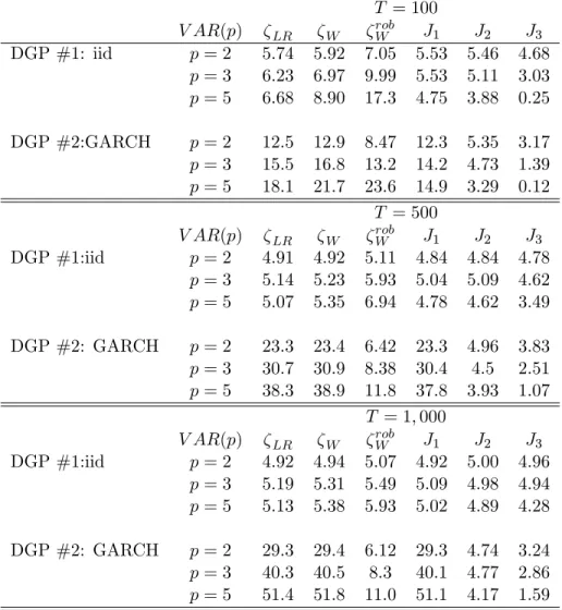
For all the tests described in the previous section, Table 1 reports the empirical rejection frequency at the 5% signi…cance level (nominal size). In theiidcase, the behavior of the six tests is rather similar, but the Wald strategy is oversized whenpincreases for small samples, and theJ3-test
(Newey-West correction) is undersized for T = 100:Results get much more worse in the presence of time varying conditional variances. With heteroskedastic data, the only test with proper size is
J2-Test, the robust-White GMM test and, to a lesser extent, the robust Wald ifT is large enough.
The other tests have large size distortions, especially the likelihood-ratio test, the non robust Wald test, and usual GMMJ1-test. Again, the J3-test (Newey-West correction) is undersized. Thus, for
macroeconomic applications we can rely either on a robust GMM or on the robust Wald if in this latter case the number of lags in the unrestricted VECM is not too large.
Table 1: Empirical size (nom. 5 percent) of common feature test statistic
T = 100
V AR(p) LR W robW J1 J2 J3
DGP #1: iid p= 2 5.74 5.92 7.05 5.53 5.46 4.68
p= 3 6.23 6.97 9.99 5.53 5.11 3.03
p= 5 6.68 8.90 17.3 4.75 3.88 0.25 DGP #2:GARCH p= 2 12.5 12.9 8.47 12.3 5.35 3.17
p= 3 15.5 16.8 13.2 14.2 4.73 1.39
p= 5 18.1 21.7 23.6 14.9 3.29 0.12
T = 500
V AR(p) LR W robW J1 J2 J3
DGP #1:iid p= 2 4.91 4.92 5.11 4.84 4.84 4.78
p= 3 5.14 5.23 5.93 5.04 5.09 4.62
p= 5 5.07 5.35 6.94 4.78 4.62 3.49 DGP #2: GARCH p= 2 23.3 23.4 6.42 23.3 4.96 3.83
p= 3 30.7 30.9 8.38 30.4 4.5 2.51
p= 5 38.3 38.9 11.8 37.8 3.93 1.07
T = 1;000
V AR(p) LR W robW J1 J2 J3
DGP #1:iid p= 2 4.92 4.94 5.07 4.92 5.00 4.96
p= 3 5.19 5.31 5.49 5.09 4.98 4.94
p= 5 5.13 5.38 5.93 5.02 4.89 4.28 DGP #2: GARCH p= 2 29.3 29.4 6.12 29.3 4.74 3.24
p= 3 40.3 40.5 8.3 40.1 4.77 2.86
6
PT decomposition under cointegration and common cycles
Lettau and Ludvigson (2001) propose a permanent-transitory representation for PVMs using a Gonzalo-Granger decomposition. This decomposition has several drawbacks. However, it corre-sponds to the Beveridge Nelson (BN hereafter) decomposition if and only if there exist in an n
dimensional model (n is the number of series in the VAR), r cointegrating vectors, and exactly
n r serial correlation common feature vectors (see Proietti, 1997; Hecq et al. 2000). Hence, the theoretical PVM requirements cannot match the Gonzalo-Granger setup, since the termSt 1 must
be present in the unpredictable linear combination of the data. In other words, in the PVM there are no linear combinations of Ytand ytalone that are unpredictable, something that is required to use the Gonzalo-Granger decomposition.
Given that PVMs entail weak form common cyclical features, we are able to decompose series into a permanent and a transitory component using the multivariate Beveridge Nelson with common cycles as developed in Hecq et al. (2000). Recall that the BN decomposition of Xt = (Yt; yt)0 in
Xt = t+ t, where the trend component denoted t, and t is a covariance stationary cyclical process, entails the use of the demeaned long-run forecast of Xt= ( Yt; yt)0:
t=Xt+ (
lim l!1
l X
i=1
~
Xt+ijt E( Xt) )
(31)
where X~t+ijt denotes the ith-step ahead forecast. Thus, the trend today represents the value to which the long-term forecast of a series converges to, when we discount its deterministic terms.
Under strong serial-correlation common features (SCCF), Proietti (1997) develops an observable permanent-transitory decomposition ofXt= (Yt; yt)0 with both common trends and common cycles such that 0 t= 0(cointegration), where is the cointegrating vector, and 0 t= 0(strong SCCF), where is the co-feature vector. Components t and t are derived in Proietti (1997). Now, in the weak-form SCCF, only a part of the cycle is annihilated by 0: Using the companion form of the VECM, Hecq et al. (2000) extend the results in Proietti (1997) and derive an observable decomposition suitable for the weak-form SCCF case, in which t= At + Bt , with 0 At = 0, but
0 B
t 6= 0 in:
Xt= t+ At + Bt : (32)
series being decomposed Bt .
From a di¤erent angle, consider a new variable:
Xt =Xt Bt = t+ At: (33)
The linear combination 0Xt = 0 t is proportional to the common trend, therefore, disregarding deterministic terms, its …rst di¤erence is unpredictable, i.e., 0 Xt is unpredictable. It is worth mentioning that this decomposition is expressed in terms of observables and only involve quantities already available from the VECM form and the estimation of common features and cointegrating vectors.
The fact that we impose the restriction that the trend is a martingale is consistent with the idea that the long-run component of asset prices is captured by a martingale, as put forth by Hansen and Scheinkman (2009). Here, however, our setup is much simpler than theirs, but it still captures the main trust in Beveridge and Nelson that, as in (31), the trend today represents the value to which the adjusted long-term forecast of a series converges to. Any deviations of prices from trend are therefore deviations of prices from fundamentals, which we label here as bubbles. Notice that the concept of a bubble here is intrinsically di¤erent from what Campbell and Shiller (1987) and West (1987) have labelled a “rational bubble” and a “speculative bubble,” respectively.
7
Empirical results
We now apply the tools covered in previous sections to two well-known economic issues. On the one hand, these are the relationship between long- and short-term interest rates, and, on the other hand, the relationship between price and dividend. We use the online series maintained and updated by Shiller at http://www.econ.yale.edu/~shiller/data.htm. Our investigations are done on those annual data spanning the period 1871-2011 (T = 141) for interest rates and on the period 1871-2010 (T = 140) for the price-dividend case. For this latter, we divide series by the consumer price index (also from Shiller´s …les) in order to obtain real prices and real dividends. Figures 1 and 2 plot the two group of series.
The four variables being I(1) according to usual unit root tests (e.g. ADF), we go next on testing for cointegration and for common cyclical features.
Figure 1: Price and dividend series (1871-2010)
0 4 8 12 16
0 200 400 600 800 1,000
80 90 00 10 20 30 40 50 60 70 80 90 00 10
REAL_DIVIDEND REAL_PRICE
Figure 2: Interest rates series (period 1871-2011)
0 4 8 12 16 20
80 90 00 10 20 30 40 50 60 70 80 90 00 10
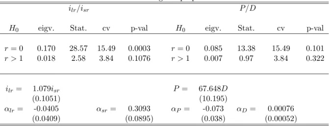
Table 2: Long run properties
ilr=isr P=D
H0 eigv. Stat. cv p-val H0 eigv. Stat. cv p-val
r= 0 0.170 28.57 15.49 0.0003 r = 0 0.085 13.38 15.49 0.101
r >1 0.018 2.58 3.84 0.1076 r >1 0.007 0.97 3.84 0.322
ilr= 1.079isr P = 67.648D
(0.1051) (10.195)
lr= -0.0405 sr= 0.3093 P = -0.073 D = 0.00076
(0.0409) (0.0895) (0.038) (0.00052)
We use a similar strategy that we have already applied in the test robW presented above but now with a di¤erent set of restrictions. In a bivariate case these can be written as
R =I2 K;
with K = I2 when testing for p = 1 (namely the bivariate white noise hypothesis) and K =
[02 (p 1) :I2]when testing for the last lag coe¢cient matrix when p > 1:This test follows a 2(4)
under the null. We have investigate on our DGPs this procedure and it emerges that it allows us to determine the correct lag length without any size distortions in the presence of heteroskedastic errors (for our DGP #2). Using this approach, we do not reject the hypothesis of VAR(2) for both economic applications.
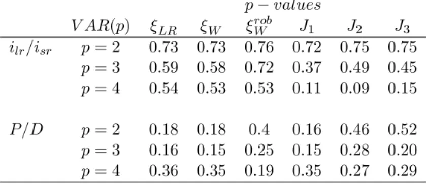
Table 3: P-values of the common feature test statistic
p values
V AR(p) LR W robW J1 J2 J3
ilr=isr p= 2 0.73 0.73 0.76 0.72 0.75 0.75
p= 3 0.59 0.58 0.72 0.37 0.49 0.45
p= 4 0.54 0.53 0.53 0.11 0.09 0.15
P=D p= 2 0.18 0.18 0.4 0.16 0.46 0.52
p= 3 0.16 0.15 0.25 0.15 0.28 0.20
p= 4 0.36 0.35 0.19 0.35 0.27 0.29
preferred testing procedure in both applications.
In both the long and short-term interest rate case and in the price-dividend analysis the null that there exists at least one weak-form common feature vector is never rejected at usual signi…cance levels. These tests do not reject the necessary rank condition behind the present value theory for both applications, which completes the …rst step of our proposed testing procedure.
We now further restrict the systems with additional constraints. First we look whether the VECMs are restricted to have a zero …rst row for lagged dependent series. For the price-dividend case thep valuesfor such an hypothesis is respectively 0.21 and 0.70 using a FIML and a robust GMM approach. If now one adds the restriction that the loading in the price equation is given by the cointegrating vector (i.e.,r^= 0:0147) p values are respectively 0.11 and 0.34 for FIML and the robust GMM.
For the long and short-term interest rates case, restricting the dynamics givesp values lower than 0.001 for FIML and 0.04 for robust GMM, hence rejecting the forecasts of the PVM on the value of the coe¢cients. Hence, for the interest rate analysis we do not further investigate the additional constraints on the coe¢cients ; and r that are theoretically given by the yield curve (see inter alia Johansen and Swensen, 2000, 2004 for a numerical example). Recall that rejecting the PVM can come from two sides: (1) …rst one can reject the rank de…ciency hypothesis and we have seen that this is not the case here; (2) some coe¢cients might not match their theoretical values. Testing (1) and (2) successively using a common feature framework helps to determine where the problem comes from. Note that in this paper we assume that the series used adequately match the theoretical counterparts in the PVMs.
pseudo-structural model estimated by FIML (standard errors in brackets):
ilr;t = 1:423
(0:715) isr;t 0(0::463193)
^
St 1+ 0:062: (0:188)
It emerges that the p-value associated with null hypothesis that the coe¢cient of isr;t is equal zero is slightly below 0.05, rejecting (9) at a 5% but not at 10% signi…cance level. Moreover the coe¢cient being positive and signi…cantly di¤erent from 1, equation (16) which discounts future expected values only, is also rejected. The negative estimated coe¢cient in front of S^t 1 is also
against the predictions of the PVM in both formulations (9) and (16).
0 2 4 6 8 10 12 14 16
80 90 00 10 20 30 40 50 60 70 80 90 00 10 10 years rate
Long-run component
Long term rate and its permanent component
-2 -1 0 1 2 3
80 90 00 10 20 30 40 50 60 70 80 90 00 10
common cycle 10 year interest rate
-200 0 200 400 600 800 1,000
80 90 00 10 20 30 40 50 60 70 80 90 00 10 common trend price
price
Price series and its permanent component
-120 -80 -40 0 40 80 120 160 200 240
80 90 00 10 20 30 40 50 60 70 80 90 00 10
common cycle price
8
Conclusion
The main contribution of this paper is to propose a novel framework for testing PV relationships in economics. Here, we stress that cointegration is simply one side of the restrictions PV relation-ships impose on the data being tested – it implies that PV equations obey certain transversality conditions. Common-cyclical-feature restrictions form the basis of the other side – they imply the existence of unforecastable errors in the stochastic di¤erence-equation generating PVMs. It is obviously preferable to test for PVMs using an integrated framework where these two types of restrictions are jointly considered. The common-feature toolkit allows the investigation of PVMs in multivariate data sets as well as the proposal of new tests for their existence.
Also, in the context of asset pricing, we propose a novel permanent-transitory (PT) decompo-sition based on Beveridge and Nelson (1981), which focus on extracting the long-run component of asset prices, a key concept in modern …nancial theory as discussed in Alvarez and Jermann (2005), Hansen and Scheinkman (2009), and Nieuwerburgh, Lustig, and Verdelhan (2010). We advance with respect to standard Beveridge and Nelson (BN) decompositions in which we compute the transitory component directly using the PVM restrictions, which amounts to impose restrictions in the short-run dynamics of the cointegrated VAR to recover the transitory component.
The techniques considered here are applied to two di¤erent data sets. The …rst contains annual long- and short-term interest rates for the US, ranging from 1871 to 2011. The second data set is for the study of the price and dividend relationship on the period 1871-2010. There is one cointegrating relationship and a weak form common feature relationship in both cases, although the analysis of interest-rate data rejects the full set of PVM restrictions. Despite that, the joint analysis of price-dividends and interest rates hints that if there is a bubble for the last global recession it came from interest rates, not from stocks. We are forced to conclude this because the long-run component of asset prices is close to current price, but the same is not true for interest rates. Indeed, the cyclical component of interest rates is now in the vicinity of its all time low – almost 200basis points.
References
[1] Alvarez, F. and U. Jermann (2005),Using asset prices to measure the persistence of the marginal utility of wealth,Econometrica, Vol. 73(6), 1977–2016.
[3] Athanasopoulos, G., Guillen, O.T.C., Issler, J.V., and F. Vahid, F. (2011),Model Selection, Estimation and Forecasting in VAR Models with Short-run and Long-run Restric-tions,Journal of Econometrics, Vol. 164(1), 116-129.
[4] Beveridge, S. and C.R. Nelson (1981),A New Approach to Decomposition of Economic
Time Series into a Permanent and Transitory Components with Particular Attention to Mea-surement of the ‘Business Cycle’,Journal of Monetary Economics, 7, 151-174.
[5] Campbell, J.Y. (1987), Does Saving Anticipate Declining Labor Income? An Alternative
Test of the Permanent Income Hypothesis,Econometrica, vol. 55(6),1249-73.
[6] Campbell, J.Y. (1991),A variance decomposition of stock returns, Economic Journal, 405, 175-179.
[7] Campbell, J.Y. and R.J. Shiller (1987), Cointegration tests and present value models,
Journal of Political Economy 95, 1062-1088.
[8] Campbell, J.Y. and A. Deaton (1989),Why is Consumption So Smooth?,The Review of
Economic Studies 56, 357-374.
[9] Campbell, J.Y, Lo, A.W. and A.C. MacKinlay (1996),The Econometrics of Financial
Markets, Princeton University Press.
[10] Candelon, B., Hecq, A. and W. Verschoor (2005),Measuring Common Cyclical
Fea-tures During Financial Turmoil,Journal of International Money and Finance, 24, 1317-1334
[11] Centoni, M., Cubadda, G. and A. Hecq (2007), Common Shocks, Common Dynamics
and the International Business Cycle,Economic Modelling, vol.24, 1, 149-166.
[12] Chow, G. (1988),Rationale versus adaptive expectations in present value models, Reserach Memorandum 328, Princeton University.
[13] Christensen, T., Hurn, S. and A. Pagan (2011),Detecting Common Dynamics in
Tran-sitory Components,Journal of Time Series Econometrics, 2011, vol. 3, issue 1.
[14] Cubadda, G. and A. Hecq (2001), On Non-Contemporaneous Short-Run Comovements,
Economics Letters, 73, 389-397.
[15] Engle, R. F. and C.W.J. Granger (1987),Co-integration and Error Correction:
Repre-sentation, Estimation and Testing,Econometrica,55, 251-276.
[16] Engle, R. F. and S. Kozicki (1993), Testing for Common Features (with comments),
[17] Engle, R. F. and J. V. Issler (1995), Estimating Common Sectorial Cycles, Journal of Monetary Economics, 35, 83-113.
[18] Engsted, T. (2002),Measures of …t for rational expectations models. Journal of Economic Surveys 16, 301-355.
[19] Gonzalo, J. and C.W.J. Granger (1995), Estimation of Common Long-Memory
Com-ponents in Cointegrated Systems,Journal of Business and Economics Statistics, 33, 27-35. [20] Hamilton, J.D. (1994), Time Series Analysis (Princeton University Press: Princeton).
[21] Hansen, L.P. (1982), Large Sample Properties of Generalized Method of Moment
Estima-tors,Econometrica, 50, 1029-1054.
[22] Hansen, L. P. and J. A. Scheinkman (2009), Long-Term Risk: An Operator Approach,
Econometrica, 77(1), 177 - 234.
[23] Hecq, A., F. Palm and J.P. Urbain (2000),Permanent-Transitory Decomposition in VAR
Models with Cointegration and Common Cycles,Oxford Bulletin of Economics and Statistics, 62, 511-532.
[24] Hecq, A., Palm, F.C., J.P. Urbain (2006),Testing for common cyclical features in VAR
models with cointegration,Journal of Econometrics, Volume 132(1), 117-141.
[25] Hecq, A., S. Laurent and F.C. Palm (2011), Pure portfolios models, RM maastricht
University.
[26] Issler, J.V. and F. Vahid. F. (2001), Common Cycles and the Importance of Transitory
Shocks to Macroeconomic Aggregates,Journal of Monetary Economics, vol. 47(3), pp. 449-475. [27] Johansen, S. (1995),Likelihood-Based Inference in Cointegrated Vector Autoregressive
Mod-els (Oxford University Press: Oxford).
[28] Johansen, S. (2000), Modelling of cointegration in the vector autoregressive model, Eco-nomic Modelling, vol. 17, 359-373.
[29] Johansen, S. and A.R. Swensen (1999), Testing rational expectations in vector
autore-gressive models,Journal of Econometrics, 93, 73–91.
[30] Johansen, S., and A. Swensen (2011), On a numerical and graphical technique for
[31] Johansen, S., and A. Swensen (2004), More on Testing Exact Rational Expectations in Cointegrated Vector Autoregressive Models: Restricted Drift Terms, Econometrics Journal, volume 7, pp. 389–397
[32] Lettau, M., and S. C. Ludvigson (2001),Consumption, Aggregate Wealth and Expected
Stock Returns,Journal of Finance, 56(3), 815—849.
[33] Lettau, M., and S. C. Ludvigson (2004),Understanding Trend and Cycle in Asset Values: Reevaluating the Wealth E¤ect on Consumption, American Economic Review, 94(1), 276— 299.
[34] Lettau, M., and S. C. Ludvigson (2010), Measuring and Modeling Variation in the Risk-Return Tradeo¤, in Handbook of Financial Econometrics, ed. by Y. Ait-Sahalia, and L. P. Hansen, vol. 1, pp. 617—690. Elsevier Science B.V., North Holland, Amsterdam.
[35] Lettau, Martin, and Sydney C. Ludvigson (2011),Shocks and Crashes, NBER Working
Paper # 16996.
[36] Phillips, Peter C B and Hansen, Bruce E. (1990),Statistical Inference in Instrumental Variables Regression with I(1) Processes,Review of Economic Studies, 57(1), pp. 99-125.
[37] Phillips, Peter C B and Loretan, Mico (1991),Estimating Long-run Economic
Equi-libria”,Review of Economic Studies, 58, pp. 407-436.
[38] Proietti, T.(1997), Short Run Dynamics in Cointegrated Systems, Oxford Bulletin of Eco-nomics and Statistics, 59,405-422.
[39] Newey, W. K. and West, K. D., (1987), A simple, positive semi-de…nite,
heteroskedas-ticity and autocorrelation consistent covariance matrix,Econometrica, vol. 55, 703–708.
[40] Ravikumar, B., Ray, S. and E. Saving (2000), Robust Wald tests in Sur systems with
adding-up restrictions,Econometrica, 68, 715-720.
[41] Vahid, F. and R.F. Engle (1993),Common Trends and Common Cycles,Journal of Applied
Econometrics, 8, 341-360.
[42] Vahid, F. and R.F. Engle (1997), Codependent Cycles, Journal of Econometrics, 80,
199-221.