Forecasting multivariate time series under present-value-model short- and long-run co-movement restrictions

(1)

Ensaios Econômicos

Escola de

Pós-Graduação

em Economia

da Fundação

Getulio Vargas

N◦ 742 ISSN 0104-8910

Forecasting Multivariate Time Series under

Present-Value-Model Short- and Long-run

Co-movement Restrictions*

Osmani Teixeira de Carvalho Guillén, Alain Hecq, João Victor Issler, Diogo Saraiva

(2)

Os artigos publicados são de inteira responsabilidade de seus autores. As

opiniões neles emitidas não exprimem, necessariamente, o ponto de vista da

Fundação Getulio Vargas.

ESCOLA DE PÓS-GRADUAÇÃO EM ECONOMIA Diretor Geral: Rubens Penha Cysne

Vice-Diretor: Aloisio Araujo

Diretor de Ensino: Carlos Eugênio da Costa Diretor de Pesquisa: Humberto Moreira

Vice-Diretores de Graduação: André Arruda Villela & Luis Henrique Bertolino Braido

Teixeira de Carvalho Guillén, Osmani

Forecasting Multivariate Time Series under Present-Value-Model Short- and Long-run Co-movement

Restrictions*/ Osmani Teixeira de Carvalho Guillén, Alain Hecq,

João Victor Issler, Diogo Saraiva – Rio de Janeiro : FGV,EPGE,

2013

39p. - (Ensaios Econômicos; 742)

Inclui bibliografia.

(3)

Forecasting Multivariate Time Series

under Present-Value-Model Short- and

Long-run Co-movement Restrictions

Osmani Teixeira de Carvalho Guillén

Banco Central do Brasil and IBMEC-RJ

Alain Hecq

Maastricht University

João Victor Issler

y

Getulio Vargas Foundation

Diogo Saraiva

Getulio Vargas Foundation

June 18, 2013

Abstract

It is well known that cointegration between the level of two variables (e.g. prices and dividends) is a necessary condition to assess the empirical validity of a present-value model (PVM) linking them. The work on cointegration,

We gratefully acknowledge the comments and suggestions given by Ricardo Brito, other partic-ipants in the 2011 SBE conference in Foz do Iguaçu, and of particpartic-ipants in the 2012 IIF Conference in Boston, where preliminary versions of this paper were presented. All remaining errors are ours. Issler thanks CNPq, FAPERJ and INCT for …nancial support. Guillén and Hecq thank INCT for …nancial support. We thank Rafael Burjack, Marcia Waleria Machado and Marcia Marcos for excellent research assistance.

y_{Corresponding address: João Victor Issler, Graduate School of Economics - EPGE, Getulio}

(4)

namely on long-run co-movements, has been so prevalent that it is often over-looked that another necessary condition for the PVM to hold is that the fore-cast error entailed by the model is orthogonal to the past. This amounts to investigate whether short-run co-movememts steming from common cyclical feature restrictions are also present in such a system.

In this paper we test for the presence of such co-movement on long- and short-term interest rates and on price and dividend for the U.S. economy. We focuss on the potential improvement in forecasting accuracies when imposing those two types of restrictions coming from economic theory.

JEL: C22, C32

(5)

1 Introduction

Using multivariate models in economics and other sciences have been proved fruitful since they entail key inter-relationships between the variables being modelled. Un-fortunately, most of these models have an abundance of free parameters, which poses a problem when they are used for forecasting, since their forecast-accuracy measures are usually outperformed by those of more parsimonious alternatives. One way to cope with this problem is to impose restrictions, reducing the number of free para-meters. In economics, this is done in two di¤erent ways within a uni…ed framework – usually, but not exclusively, a vector autoregressive (VAR) model. The …rst is to impose long-run relationships among the series being modelled when they trend over time, i.e., to impose cointegration restrictions; see Engle and Granger (1987). The second is to impose similarities in their short-run dynamics, i.e., to impose common-cycle restrictions either in weak or in strong form; see Engle and Kozicki (1993), Vahid and Engle (1993) and Hecq et al. (2000, 2006).

The extensive work on cointegration (e.g. Engle and Yoo, 1987 or Reinsel and Ahn, 1992, and all the literature that followed) has shown that considering and im-posing long-run relationships leads to forecasting gains compared to the model in …rst di¤erences (see also Clements and Hendry, 1998 or Ho¤man and Rasche, 1996,

inter alia). However, less than a handful of papers (e.g., Issler and Vahid, 2001, Vahid and Issler, 2002, Anderson and Vahid, 2011) have investigated whether addi-tional short-run co-movement restrictions generate better forecasts. Moreover, only recently have Athanasopoulos et al. (2011) compared the relative importance of these two types of restrictions using simulations and real data, their results showing that existing short-run restrictions have a greater potential to improve forecast accuracy compared to cointegration restrictions.

(6)

examples where the short-run behavior of consumption and income is restricted by liquidity-contraint models or by optimal-consumption models.

More importantly, short-run restrictions are implied by the present-value model studied here. So are long-run restrictions, but Campbell and Shiller (1987) have only stressed the fact that cointegration between the level of two variables (labeledYtand

ytin this paper) is a necessary condition for the validity of a present-value model (PV

and PVM, respectively, hereafter) linking them.1 _{Hence, it is often overlooked that}

another necessary condition for the PVM to hold is that the forecast error entailed by the PV model is orthogonal to the past. We refer to Hansen and Sargent (1981, 1993) and Baillie (1989) for initial work on rational expectations linked to PVMs, and Johansen and Swensen (1999, 2004, 2011), and Johansen (2000), for a recent fresh look on the subject. The basis of this result is the use of rational expectations

in forecasting future values of variables in the PVM.

Indeed, PVMs arise from a …rst-order stochastic di¤erence equation, where its error term must be unforecastable regarding past information, i.e., it must have a zero conditional expectation. If this fails, the PV equation will not be valid, since it will contain an additional term capturing the (non-zero) conditional expected value of all future error terms. Cointegration imposes the transversality condition allowing to discard the limitI(0)combination ofYtandyt. The existence of an unforecastable

linear combination of theI(0) series in the di¤erence equation guarantees that the dynamic behavior of the variables in the PVM is consistent with theory. Since we need both conditions to validate PVMs, it is ideal to work with an integrated econometric framework encompassing the joint existence of these two phenomena.

This is the starting point this article. We …rst show that PV relationships entail a weak-form common feature restriction, as in Hecq et al. (2006) and in Athana-sopoulos et al. (2011), for the vector error-correction model (VECM) forYt and yt.

It also implies a polynomial serial correlation common feature relationship (Cubadda

1_{Examples of}_Y

tandytare, respectively, prices and dividends for a given asset, long- and

(7)

and Hecq, 2001) for the VAR representation for yt and the cointegrating

relation-shipYt yt:These represent short-run restrictions on the dynamic system for these

variables. Once we cast the PVM in these terms, it is straightforward to apply the toolkit of the common-feature literature for inference and testing, which has supe-rior results vis-a-vis standard methods. This is the …rst original contribution of this paper.

Our second contribution relates to forecasting series that are subject to PVM re-strictions, which has a wide application in macroeconomics and …nance. We bene…t from our previous theoretical results, especially regarding the existence of common-cyclical features in its various forms. As is well known, there has been previous work showing the forecasting bene…ts when the short-run dynamics of the system is con-strained for stationary data (Vahid and Issler, 2002), and when it is concon-strained for data subject to long- and short-run restrictions (Issler and Vahid, 2001, Anderson and Vahid, 2011, and Athanasopoulos et al., 2011). The reason why appropriate common-cycle restrictions improve forecasting is because they …nd linear combina-tions of the …rst di¤erences of the data that cannot be forecast by past information. This embeds natural exclusion restrictions preventing the estimation of useless pa-rameters, which would otherwise contribute to the increase of forecast variance with no expected reduction in bias. After all, forecast models should not try to forecast the unforecastable? The whole issue is obviously parsimony, but the exclusion re-strictions are chosen in a way that is aligned with the …nal objective – to forecast the series in the system – eliminating parameters that go against that.

We show the relevance of the issues discussed above in an empirical exercise in-volving two sets of …nancial series. The …rst contains annual long- and short-maturity interest rates for the U.S. economy. The second contains real price and dividend for the S&P composite index and the real risk-free rate. Both data sets were extracted from the online library maintained and updated by Shiller

(8)

the latter with additional speci…c parameter restrictions implied by economic theory. Each layer corresponds to a speci…c restricted representation for the reduced form VAR. Forecast-accuracy measures across representations are compared to evaluate the bene…ts of imposing each set of restrictions. Since the all restricted representa-tions forecast the …rst-di¤erence of the data, but the VAR forecasts their level, we transform the VAR forecasts errors to be equivalent to …rst-di¤erence errors in order to make the …nal comparisons.

Our last contribution is to devise a testing strategy for PV restrictions in macro-economics and …nance incorporating more than 20 years of research on this topic. We cover several important issues. First, how to choose consistently the lag length of the VAR. Second, testing for cointegration, common cycles and weak-form common cycles. We discuss a multivariate approach based on the likelihood ratio test (canon-ical correlation analysis) and a single-equation heteroskedasticity robust approach (GMM). Part of our suggested strategy relies on Monte-Carlo simulation results. Fi-nally, we also suggest integrated approaches estimating jointly the lag length of the VAR and long-run and short-run parameters as in Athanasopoulos et al. (2011), and an alternative estimating jointly long-run and short-run parameters as in Centoni, Cubadda and Hecq (2007).

(9)

2 Present-value models

2.1 Basic representation in levels, long- and short-run

co-movement

Consider the present value equation:2

Yt= (1 ) 1

X

i=0

i

Etyt+i; (1)

which states thatYt is a linear function of the present discounted value of expected

future yt, where Et( )is the conditional expectation operator, using information up

totas the information set. In most casesYtandytareI(1)variables. Examples ofYt

andytinclude, respectively: long and short-term interest rates, real stock prices and

real dividends, personal consumption and disposable income, etc. (see the survey Engsted, 2002). In this subsection, it is assumed constant expected returns with a discount factor = ₁₊1_r: The coe¢cient is a factor of proportionality. For example,

= =(1 ) in the price-dividend relationship; = 1 for the interest rates case and the link with the discount factor is given by the term structure of the interest rates (see, inter alia, Chow, 1984; Campbell and Shiller, 1987; Johansen and Swensen, 2011). The choice of only impacts the value of the cointegrating vector. Hence, here, in what follows, we set its value equal to = =(1 ), such that:

Yt= 1

X

i=0

i

Etyt+i: (2)

Following Campbell and Shiller (1987), the actual spread is de…ned as:

St Yt

1 yt; (3)

2_{For simplicity, we do not inlcude a constant term at this level of presentation as some papers}

(10)

where St is I(0) if Yt and yt are cointegrated. Subtracting ₁ yt from both sides of

(2) produces the theoretical spread S0 t:

St0 = 1

1

X

i=1

i

Et yt+i: (4)

This shows that series must be theoretically cointegrated because the right-hand side is a function of I(0) terms with exponentially decreasing weights. Further, subtracting EtYt+1 = P

1 i=0

i

Etyt+i+1 from Yt in (4), we obtain:

Yt = EtYt+1+ yt: (5)

From (5), if one adds and subtracts Yt; leading to Yt = Et Yt+1 + Yt+ yt or (1 )Yt= Et Yt+1+ yt, one …nally obtains:

S_t00 =

1 Et Yt+1: (6)

Equation (6) gives the spread as a function of one-step ahead forecasts of Yt+1. We

can always perform the following decomposition:

Yt+1 =Et Yt+1+ ( Yt+1 Et Yt+1)

| {z }

ut+1

: (7)

Plugging (7) into (6), and lagging the whole equation by one period we haveSt 1 = 1 Yt+ut or alternatively,

Yt= 1

(11)

whereut(orvt = 1 ut) is orthogonal to the past in expectation. From (8) we also

obtain:

(1 )St 1 = Yt+ (1 )ut (9)

St 1 Yt 1+

1 yt 1 = Yt Yt 1+ 1 yt 1 yt + (1 )ut

St 1 = St+

1 yt+ (1 )ut

which gives

St = 1

St 1

1 yt+"t (10)

with "t= (1 )ut.

As stressed by Campbell (1987), in the context of saving, equation (10) plays a very important role: it is the …rst order stochastic di¤erence equation that generates the PVM. There are two important conditions to go from (10) to (4): cointegration delivers the transversality condition lim

k!1 k

Et(St+k) = 0, whereas unforecastability

of"tregarding the past, i.e.,Et("t+1) = 0, ensures that there is no additional term in

the right-hand side of (4) invalidating it. The …rst represents a long-run restriction betweenYtandyt. The second restricts the dynamics of the stationary representation

of the system, making St and yt speci…c functions of their own past alone. Thus,

they can be viewed as short-run restrictions on the behavior ofStand yt. These are

exactly the types of restrictions studied in the common-cycle literature. Therefore, applying thetoolkit developed there allows a fresh view of PVMs as we show below.

Remark 1. Johansen and Swensen (2011) discuss the properties of the three spreads

St, S 0

t, and S 00

t. Their setup is slightly di¤erent than ours, since, in (1), they

de-…ne the present-value relationship to be Yt = P 1 i=1

i

Etyt+i instead of Yt = (1 )P1_i₌₀ iEtyt+i, i.e., they discount only future values ofyt and not its current value.

(12)

we shall see in the next section. For that reason, some of our results are not identical to those in Johansen and Swensen (2011).

2.2 Common-cyclical feature restrictions: VARs and VECMs

Assume that the bivariate system for the I(1) series (Yt; yt)0 follows a VAR(p) in

levels, and that St = Yt yt is the stationary error-correction term. In the

price-dividend case = ₁ : The corresponding vector error-correction model (VECM) representation is given by:

Yt

yt

!

= 1

Yt 1

yt 1

!

+:::+ p 1

Yt p+1

yt p+1

!

+ 1

2

!

St 1+ 1t 2t

!

; (11)

where we assume that the disturbance terms are white noise and that conditions for avoiding I(2)-ness are met. The is are the short-run coe¢cient matrices, and 1

and 2 are the loadings on the error-correcting term.

As is well known, PV relationships imply restrictions on dynamic models of the data. Campbell and Shiller (1987) and others have exploited the fact that VARs have cross-equation restrictions. Here, however, we exploit a di¤erent nature of these restrictions – the fact that there are also reduced-rank restrictions for the VECM (11).

Proposition 1. If the elements of (Yt; yt)0 obey a PV relationship as in (9), i.e.,

St 1 = ₁ Yt+ut, then, their VECM obeys a weak-form common feature

relation-ship (see Hecq et al., 2006, and Athanasopoulos et al., 2011): there exists a 1 2

vector 0

such that 0

1 = 0 2 = ::::= 0 p 1 = 0, but 0 1 2

!

6= 0: Moreover,

0

= (1 : 0); the …rst row of every i; i= 1:::p 1, must be zero, and the following

restriction must also be met: 1 = 1 .

The usual cross-equation restriction within the VAR and proposed by Campbell and Shiller (1987) can also be seen from a transformed VAR on St and yt; see

(13)

representation we use C =

"

1 0 1

#

, the 2 2 nonsingular matrix formed by

stacking the transpose of the cointegrating vectorh 1 i and the selection vector

h

0 1 i, such that C Yt yt

!

= St

yt

!

. Premultiplying both sides of (11) by

C, and solving forSt and yt, we obtain:

St

yt

!

= 11(L) 12(L)

21(L) 22(L)

!

St 1

yt 1

!

+ 1t

2t

!

(12)

where 11(L) and 21(L) are polynomials of order p 1 and 12(L) and 22(L)

are polynomials of order p 2: Indeed, one important issue is to note is that the transformed VAR (12) is a VAR of order p both inSt and in yt in which the two

coe¢cients of yt p are zero. Cross-equation restrictions for the system are imposed

on the coe¢cient matrices of (L) = 11(L) 12(L)

21(L) 22(L)

!

= 1+ 2L+ pLp 1 in

(12).

We have the following proposition.

Proposition 2. A PVM as in (10), i.e.,St = 1St 1 ₁ yt+"t, implies a

polyno-mial serial-correlation common feature relationship (see Cubadda and Hecq, 2001) for the transformed VAR (12): there exists a vector~0

0 such that~

0

0 2 =::::= ~

0

0 p = 0,

with ~0_{0 1} = ~0₁ 6= 0: Moreover in the PVM ~₀0 = (1 : ₁ )and ~0₁ = ( 1 _{: 0)}_:

Thus, a PVM entails cointegration and additional orthogonality conditions as-sociated with reduced rank restrictions in VECMs or transformed VARs. One of the possible explanations for observing a rejection of the PVMs is the use of cross-equation restrictions that impose both reduced-rank restrictions and particular values on the parameters. Misspeci…cations such as proxy variables or measurement errors can a¤ect the value of the parameters, leaving una¤ected the reduced-rank restric-tions. As an example, instead of the PV representation Yt = (1 )P

1 i=0

i

Etyt+i

(14)

expected value ofyt such thatYt=P 1 i=1

i

Etyt+i:3 This slight change is not

innocu-ous as we show next. To see that, apply the algebra used before toYt =P 1 i=1

i

Etyt+i

to obtain the following expressions:

Yt = yt+ 1

St 1+ut; (13)

where 0

= (1 : 1)and 1 =

1

in Proposition 1. (14)

St =

1

(1 ) yt+ 1

St 1 +vt; (15)

where ~0

0 = (1 :

1

1 ) and ~ 0

1 = (

1

: 0) in Proposition 2. (16)

What emerges now is that the unpredictable linear combinations involve three vari-ables: Yt, yt, and St, both in the VECM and the transformed VAR. Moreover

the values of the parameters are now di¤erent from before – the weights used in the linear combinations (13) and (15) di¤er from the ones in (8) and (10), respectively.

Put di¤erently, regarding the use of Yt = P 1 i=1

i

Etyt+i versus Yt = (1 )P1

i=0

i

Etyt+i, respectively, yields the following orthogonality conditions for each

speci…c di¤erence equation:

Et 1 Yt+ yt 1

St 1 = 0, vs. Et 1 Yt 1

St 1 = 0,

Et 1 St+ 1

(1 ) yt 1

St 1 = 0, vs. Et 1 St+

1 yt

1

St 1 = 0.

Despite the di¤erences in parameter values in the linear combinations above, the existence of a reduced-rank model is not a¤ected by how one writes the PV equation linking Yt and yt. Hence, the reduced-rank properties of the VECM and of the

transformed VAR are invariant to this choice: in both cases, there exists weak-form common features for the VECM and the PSCCF for the transformed VAR.

3_{Johansen and Swensen (2011) as well as Campbell, Lo and Mackinlay (1996) use that}

(15)

2.3 Constant versus variable expected returns: levels versus

logs

Campbell and Shiller’s (1987) model for the level of prices(Yt)and dividends(yt)is consistent with a very restrictive assumption – that the expected return of a given stock is constant through time:

Et[Rt+1] =R; (17)

where

Rt+1

Pt+1+Dt+1

Pt

1; (18)

wherePt and Dt denote, repectively, the price and the dividend of a given stock.

In two subsequent papers, Campbell and Shiller (1988a,b) developed an alterna-tive representation for prices and dividends, in which (17) needs not hold, so being consistent with the idea of time-varying returns. This alternative representation uses the logarithm of prices and dividends:

ht+1 log(1 +Rt+1) = log(Pt+1+Dt+1) log(Pt); (19)

arriving at:

ht+1 =pt+1 pt+ log(1 + exp(dt+1 pt+1)); (20)

where lower-case variables represent the respective logarithmic transformation of the original variable.

They use a …rst-order taylor expansion in (20), to get:

(16)

where _(1+exp(1_{d p}₎₎, and d p is the average across time of dt+1 pt+1, and

k log( ) (1 ) log(1= 1):

Notice that we can solve (25) for(dt pt), yielding an exact stochastic …rst-order

di¤erence equation for it,

(dt pt) = k+ht+1 dt+1 (pt+1 dt+1) +"t+1; (26)

where "t+1 is an approximation error. Under the assumption that Et("t+j) = 0,

for all j > 0, equation (26) can be solved forward to yield a logarithmic version of equation (4):

dt pt=

k

1 +Et 1

X

j=0

j_[_h

t+1+j dt+1+j]: (27)

Campbell and Shiller (1988a) argue that “there is no economic content in equa-tion (27)”. To get economic content they impose a restricequa-tion on the behavior and dynamics ofht:

Etht+1 =Etrt+1+c; (28)

i.e., that the excess-return of a stock, vis-a-vis the real risk-free ratert, is constant.4

Ifrt is observable, (27) and (28) yield a testable econometric model:

dt pt=

c k

1 +Et 1

X

j=0

j_[_r

t+1+j dt+1+j]: (29)

2.4 Common-cyclical feature restrictions: the logarithmic

version

To test the log-linear present value model embedded in (29), we use the tri-dimensional system forXt = (pt; dt; rt)0. Notice …rst that (28) implies that rt is I(0), given that

ht = is I(0). This yields the …rst cointegrating vector for the system in Xt. Given

that rt is I(0), from (29) dt pt is I(0) as well, yielding the second cointegrating

vector in the system.

4_{Equation (}₂₈_{) implies the existence of a common cycle for}_h

(17)

The VECM(p 1) reads as: 2 6 4 pt dt rt 3 7 5 = 2 6 4 1 4 2 5 3 6 3 7 5 "

(dt 1 pt 1)

rt 1

# + 0 B @ a1

11 a112 a113

a1

21 a122 a123

a1

31 a132 a133

1 C

A Xt 1+

+

0 B @

ap₁₁1 ap₁₂1 ap₁₃1 ap₂₁1 ap₂₂1 ap₂₃1 ap311 ap321 ap331

1 C

A Xt p 1+ t (30)

Disregarding an irrelevant constant term, the PVM implies thatEt 1[ht rt] = 0.

From equation (25), we can approximate ht as ht = pt + (1 )(dt 1 pt 1).

Consequently in the VECM, if we pre-multiply the system (30) by 0 1 , in order to obtain an expression forht rt, we must have:

0 1 Xt

| {z }

pt rt

= (1 )(dt 1 pt 1) +rt 1+ 0 1 t (31)

which is equivalent to

pt+ (1 )(dt 1 pt 1)

| {z }

ht

rt= 0 1 t, (32)

which implies Et 1[ht rt] = 0: Those theoretical conditions restrict the VECM

parameters as follows:

0 1

0 B @

ai

11 ai12 ai13

ai

21 ai22 ai23

ai

31 ai32 ai33

1 C

A = 0; i= 1; :::; p 1, and, (33)

0 1 2 6 4 1 4 2 5 3 6 3 7 5 "

(dt 1 pt 1)

rt 1

#

= ( ₁ ₃)

| {z }

(1 )

(dt 1 pt 1)

+( ₄ ₆)

| {z }

1

(18)

The last set of restrictions in (34) are:

1 =

3 (1 )

, and, (35)

4 = 6

+ 1

: (36)

Given the estimates of 3, 6, and _(1+exp(1_{d p}₎₎, we can obtain the corresponding

values of 1 and 4, consistent with (29). We now summarize these results with the

following proposition.

Proposition 3. If the elements in Xt = (pt; dt; rt)0 obey a PVM as in (29) and

(28), the latter leading to ht=rt+"t, where ht = pt+ (1 )(dt 1 pt 1), and

Et 1["t] = 0, then, their VECM obeys a weak-form common feature relationship

(Hecq et al., 2006, and Athanasopoulos et al., 2011): there exists a 1 3 vector

0

= 0 1 , such that 0

0 B @

ai

11 ai12 ai13

ai

21 ai22 ai23

ai

31 ai32 ai33

1 C

A = 0; i = 1; :::; p 1, implying

that the …rst row of

0 B @

ai

11 ai12 ai13

ai

21 ai22 ai23

ai

31 ai32 ai33

1 C

A is proportional to the last row (1= ); that

0

2 6 4

1 4

2 5

3 6

3 7

56= 0, with …rst-row elements being restricted as follows: ₁ = 3 (1 )_,

and 4 = 6+1.

Finally, as was the case for the same series in levels, i.e.,PtandDt, slight changes

on the assumptions of when dividends are accrued (begining, middle or end of period

t) in‡uence the short-run parameter restrictions imposed on the multivariate system forXt= (pt; dt; rt)0. As we noted above, this is not a trivial issue, especially because

(19)

what are the appropriate short-run parameter restrictions that should be imposed in PVMs. Although short-run parameter restrictions are not invariant to changes in dividen policy, rank restrictions discussed in Propositions 1 and 3, are invariant to them. We take this explicitly into account in devising the forecast models considered n the forecast experiment.

3 In-sample analysis of the data used in the

fore-cast experiment

We analyze here three di¤erent data sets which are later used in the forecast exper-iment. The …rst includes the levels of interest rates with long and short maturities, labelled ilr and isr, respectively. The second includes the level of real price and

div-idend for the S&P composite index, labelled Pt and Dt, and the last involves the

logarithmic transformation of prices and dividends, pt = lnPt and dt = lnDt, with

the inclusion of the real risk-free rate, labelled rt. Data is collected for the period

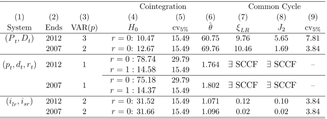
1871-2012 by Shiller. Results are presented in Table 1.

For each of them, we use the Hannan-Quinn information criteria to determine the lag length of the VAR in levels. This is reported in the third column of Table 1. Columns (4), (5) and (6) refers to as the cointegration analysis. We do not reject the null of no long-run relationships when the levels are used but the sensible value of the discount factor may lead to the conclusion that we have a power issue. There is a clear indication of cointegration for the interest rates as well as for prices/dividends in logs. Notice that we should have found two cointegrating vectors for the system with (pt; dt; rt)0. Strictly speaking, we only found one cointegrating vector at 5%

signi…cance, albeit the test statistics is very to close to the critical value at that level. So, imposing two vectors could be a possibility. As far as common-cyclical features are concerned, results in columns (7) to (9) show a clear indication of weak-form common features for interest rates; we also conclude that there is a common feature vector for the system (Pt; Dt)0 if we use the robust GMM test J2. For the

(20)

Table 1: Long and short-run properties of the series in the forecast experiment

Cointegration Common Cycle

(1) (2) (3) (4) (5) (6) (7) (8) (9)

System Ends VAR(p) H0 cv5% ^ LR J2 cv5%

(P_t; D_t) 2012 3 r= 0: 10.47 15.49 60.75 9.76 5.65 7.81 2007 2 r= 0: 12.67 15.49 69.76 10.46 1.69 3.84 (p_t; dt; rt) 2012 1

r= 0 : 78:74

r= 1 : 14:58

29.79

15.49 1.764 9 SCCF 9 SCCF –

2007 1 r= 0 : 75:18

r= 1 : 14:37

29.79

15.49 1.802 9 SCCF 9 SCCF – (i_lr; i_sr) 2012 2 r= 0: 31.52 15.49 1.071 0.12 0.10 3.84

2007 2 r= 0: 31.66 15.49 1.096 0.02 0.02 3.84

always exist SCCFs.

Therefore, we were able to …nd empirically that data subject to the theory of PVMs conform to some of the restrictions implied by theory. In our forecast experi-ment below, we ask a di¤erent question: whether or not imposing these restrictions in unrestricted multivariate models for that same data leads to an improvement of standard forecast-accuracy measures. This experiment have not only bearings on theory, but on practical issues as well.

4 Out-of-sample forecasting

4.1 Forecasting strategies imposing di¤erent co-movement

restrictions

We describe next the di¤erent forecast strategies used in this paper, each of them imposing a di¤erent set of co-movement restrictions on the unrestricted VAR, our benchmark forecasting model:

(21)

2. VECM(HQ-PIC): This is the VECM possibly restricted (but not necessar-ily) by cointegration and/or by weak-form serial-correlation common features: select jointlyp, the rank of the short-run matrices, and the cointegrating rank, by the combination of the use of the posterior information criterium (PIC) and the HQ criterium as suggested by Athanasopoulos et al. (2011), further esti-mating all parameters by their two-step conditional ML. Forecast the variables in the system up toh periods ahead.

3. VECM(HQ-J):This is the VECM using solely the PVM-cointegration restric-tion. Select p by the HQ criterium, impose the cointegrating-rank restriction consistent with the PVM. Conditional on that restriction, estimate the coin-tegrating vector consistently (Johansen, 1991), further performing conditional ML estimation using estimated cointegrating vectors. Forecast the variables in the system up toh periods ahead.

4. VECM(HQ)Rank: This is the VECM using solely the PVM cointegration and weak-form serial-correlation-common-feature rank restrictions. Selectpby the HQ criterium (Athanasopoulos et al., 2011), where we impose the rank restrictions for cointegration and weak-form serial-correlation-common-feature consistent with the PVM. Estimate all parameters by conditional ML and forecast the variables in the system up toh periods ahead.

5. PV model: This is the VECM using the PVM cointegration and weak-form serial-correlation-common-feature rank restrictions, in addition to the theoret-ical restrictions discussed in Propostion 2. Select p by the HQ criterium, es-timate all parameters by conditional ML, imposing the restrictions outlined in Proposition 2, where we use the cointegrating vector estimate of b (T -consistent) to constrain _b1 = 1_bb = 1=b. From the quasi-structural form

we recover the reduced-form and forecast the variables in the system up to h

periods ahead.

6. Log PV model: This is the VECM for Xt = (pt; dt; rt)0, using the PVM

(22)

in addition to the theoretical restrictions discussed in Propostion 4. Select p

by the HQ criterium. Estimate the last two reduced-form equations under the previous restrictions and set_b _(1+exp(1_{d p}₎₎, where d p is the time-average of dt pt. With the last two equations of reduced-form estimates and b, we

assemble the quasi-structural form, recover the reduced-form, and then fore-cast the variables in the tri-variate system forXt = (pt; dt; rt)0 up to h periods

ahead. Loss functions here are computed vis-a-vis the logged variables, i.e., vis-a-vis the variables in Xt= (pt; dt; rt)0.

(23)

atheoretical (reduced form) econometric models.5

For the empirical analyses we use the online series maintained and updated by Shiller at http://www.econ.yale.edu/~shiller/data.htm. The estimation details for the forecasting models are as follows. First, we divide our total sample in “estimation sample” and “forecasting sample.” Since the great recession (2008-2009) has had a huge in‡uence on asset prices and on the prices of bonds (interest rates), we considered two separate forecast samples: the …rst ending in 2007, just prior to the great recession, and the second ending in 2012, with all available information up to now. We set h = 12 in the forecasting exercise. This enables measurement of short- and medium-term forecast accuracy (h between 1 and 5 years) as well as long term (h > 10 years). When forecasting until 2007, we have 70 observations for the estimation sample (from 1871-1940) and 67 observations for the forecasting sample (1941-2007).6 _{When forecasting until 2012, the estimation sample has 75}

observations (from 1871-1945) and 67 observations for the forecasting sample (1946-2012). Estimation is performed with a rolling window, kept constant throughout the out-of-sample exercise.

The forecast accuracy of all restricted models are compared to that of the VAR in levels. We use the ratio of the root-mean-squared-forecast error for each model (or variable in them) vis-a-vis that of the VAR in levels – our benchmark:

RRM SF E_hM = RM SF E M h

RM SF EV AR h

; (37)

where RRM SF EM

h is the root-mean-squared-forecast error (RMSFE) statistic of

modelM, relative to that of the unrestricted VAR, forh step-ahead forecasting. All comparisons are made using the embed …rst-di¤erence forecast errors.

We want to be able to distinguish the forecast accuracy of models (1)-(6), asking whether their accuracy measures are statistically equal or not. We do this using the

5_{About the dispute between reduced- and structural-form in econometrics, see the recent paper}

by Keane (2010) and further comments on it.

6_{Notice that, the number of out-of-sample observations di¤ers for}_h_{= 1}_, _h_{= 2}_{, all the way to}

(24)

unconditional predictive ability test of Giacomini and White (2006), comparing each model M with the unrestricted VAR, and comparisons across all other models as well.

4.2 Forecasting results

We have forecast results for three di¤erent data sets. The …rst is regarding the levels of interest rates with long and short maturities, labelled ilr and isr, respectively,

where theory assumes the long rate to be the expected PV of the discounted short rate. The second is regarding the level of real price and dividend for the S&P composite index, labelled Pt and Dt, where price should be the expected PV of

the discounted dividend stream. The last involves the logarithmic transformation of prices and dividends, pt = lnPt and dt = lnDt, respectively, which PV analysis

requires the inclusion of the real risk-free rate, labelled rt.

We computed the relative measure of forecast accuracy (RMSFE) of model M

vis-a-vis the VAR, described in (37). Since the all restricted representations (models (2)-(6)) forecast the …rst-di¤erence of the data, but the VAR (model (1)) forecasts their level, we transform the VAR forecasts errors to be equivalent to …rst-di¤erence errors in order to for the ratio in (37). Following the empirical …nancial literature, which relies much more on individual-data results, we focus on forecast measures for the individual variables instead of those for the system as a whole – a good example being Patton, Ramadorai, and Streat…eld (2013).

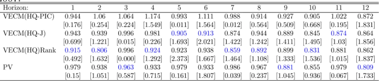
In Tables 2 through 5, we present forecast results for isr and ilr. When we

(25)

Table 2: Relative RMSFE of restricted models vs VAR for isr. Forecast period up

to 2007.

Horizon: 1 2 3 4 5 6 7 8 9 10 11 12 VECM(HQ-PIC) 1.058 1.056 1.014 1.057 1.051 1.206 1.005 0.886 0.907 0.955 0.908 0.842

[0.27] [0.216] [0.013] [0.124] [0.246] [1.409] [0.001] [0.795] [0.63] [0.122] [0.59] [1.208] VECM(HQ-J) 0.952 0.955 0.997 0.919 0.949 0.96 0.927 0.892 0.845 0.88 0.86 0.84

[0.906] [0.839] [0.011] [1.452] [0.9] [0.58] [2.119] [1.56] [1.517] [1.3] [1.345] [1.317] VECM(HQ)Rank 0.952 0.871 0.901 0.987 0.931 0.958 0.955 0.914 0.894 0.886 0.865 0.878

[0.948] [1.122] [1.317] [0.471] [0.931] [0.341] [1.971] [1.593] [1.597] [1.406] [1.367] [1.273] PV 0.946 0.923 0.932 0.956 0.923 0.896 0.874 0.895 0.804 0.801 0.81 0.801

[1.372] [0.843] [0.965] [1.131] [0.836] [1.191] [1.514] [1.196] [1.549] [1.328] [1.235] [1.248]

Ratio of root-mean-squared-forecast error (RMSFE) of model in each row to that of the VAR in levels, transformed to …rst di¤erences. Best Models in blue. Denotes rejection of the null of equal forecast accuracy at the 10% level, according to the Giacomini and White (2006) test. The number in [] is the test statistic and the critical value is equal to 2.705.

Denotes rejection of the null of equal forecast accuracy at the 5% level, according to the Giacomini and White (2006) test. The number in [] is the test statistic and the critical value is equal to 3.8415

Denotes rejection of the null of equal forecast accuracy at the 1% level, according to the Giacomini and White (2006) test. The number in [] is the test statistic and the critical value is equal to 6.6349.

Table 3: Relative RMSFE of restricted models vs VAR forilr. Forecast period up to

2007.

Horizon: 1 2 3 4 5 6 7 8 9 10 11 12

VECM(HQ-PIC) 0.944 1.06 1.064 1.174 0.993 1.111 0.988 0.914 0.927 0.905 1.022 0.872 [0.176] [0.254] [0.224] [1.549] [0.011] [1.564] [0.012] [0.564] [0.509] [0.668] [0.195] [1.831] VECM(HQ-J) 0.943 0.939 0.996 0.981 0.905 0.913 0.874 0.944 0.889 0.845 0.874 0.864

[0.699] [1.221] [0.015] [0.226] [1.693] [2.021] [1.422] [1.242] [1.411] [1.495] [1.03] [1.856] VECM(HQ)Rank 0.915 0.806 0.996 0.924 0.923 0.938 0.859 0.892 0.899 0.831 0.881 0.862

[0.492] [1.632] [0.000] [1.292] [2.373] [1.667] [1.464] [1.108] [1.333] [1.536] [1.015] [1.837]

PV 0.979 0.938 0.963 0.933 0.979 0.933 0.986 0.967 0.881 0.855 0.979 0.809

[0.15] [1.051] [0.587] [0.715] [0.161] [1.807] [0.039] [0.237] [1.045] [0.936] [0.067] [1.733] See Notes of Table 2.

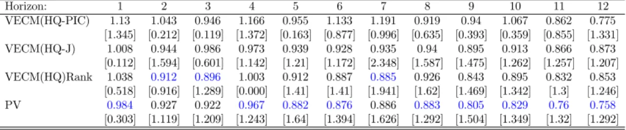
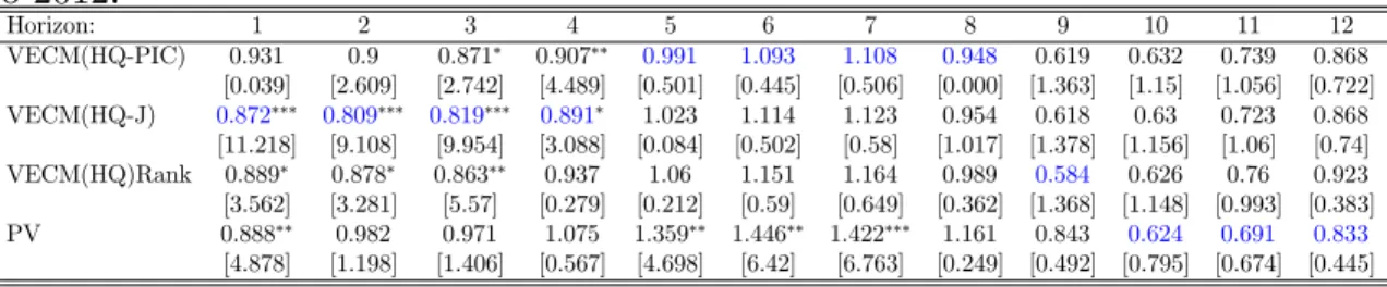
performs well in the medium- to long-horizon. Thus, for interest-rate forecasts, we conclude that the PV model (5) and strategy (4, VECM(HQ)Rank) perform really well. Despite that, it should be noted that no strategy has a forecast performance that is statistically superior to that of the VAR, the exception being strategy (2, VECM(HQ-J)) at the 7-year-ahead horizon.

In Tables 6 through 9, we present forecast results for prices and dividends for the level of the S&P 500 portfolio, Pt and Dt. In forecasting Pt, the PV model

(5) performed really well regardless of the forecast sample (2007 or 2012), although its performance in the short horizon up to 2007 was beaten by that of strategy (2, VECM(HQ-PIC)) and strategy (3, VECM(HQ-J)). RegardingDt, for short horizons,

(26)

Table 4: Relative RMSFE of restricted models vs VAR for isr. Forecast period up

to 2012.

Horizon: 1 2 3 4 5 6 7 8 9 10 11 12

[0.112] [1.594] [0.601] [1.142] [1.21] [1.172] [2.348] [1.587] [1.475] [1.262] [1.257] [1.207] VECM(HQ)Rank 1.038 0.912 0.896 1.003 0.912 0.887 0.885 0.926 0.843 0.895 0.832 0.853

[0.518] [0.916] [1.289] [0.000] [1.41] [1.41] [1.941] [1.62] [1.469] [1.342] [1.3] [1.246] PV 0.984 0.927 0.922 0.967 0.882 0.876 0.886 0.883 0.805 0.829 0.76 0.758

Table 5: Relative RMSFE of restricted models vs VAR forilr. Forecast period up to

2012.

Horizon: 1 2 3 4 5 6 7 8 9 10 11 12

[2.144] [1.472] [4.44] [0.238] [1.74] [2.646] [3.089] [0.943] [1.117] [1.351] [0.706] [1.999] VECM(HQ)Rank 0.927 0.823 1.011 0.95 0.957 0.948 0.94 0.937 0.922 0.918 0.916 0.888

[0.216] [1.468] [0.292] [1.03] [2.219] [2.006] [2.561] [0.944] [1.233] [1.445] [0.765] [1.876]

PV 0.937 0.881 0.965 0.939 0.982 0.97 0.998 0.959 0.899 0.882 0.871 0.849

horizon. Thus, for Pt and Dt, we conclude that PV model (5) and strategies (2,

VECM(HQ-PIC)) and (3, VECM(HQ-J)) are the best.

In Tables 10 through 13, we present forecast results forptanddt. When forecasts

are carried out until 2007, the best model for pt is strategy (3, VECM(HQ-J)),

while there is no clear best strategy fordt: for short horizons the log PV model (6)

performs well, for the medium horizons strategy (3, VECM(HQ-J)) is best, while for long horizons strategy (4, VECM(HQ)Rank) is the best one. For the full forecast sample up to 2012, the best model for pt is strategy (3, VECM(HQ-J)), while for

dt log PV model (6) performs well for h = 1, strategy (3, VECM(HQ-J)) is best

for h = 2;3, while for long horizons strategy (4, VECM(HQ)Rank) is the best one. Thus, we conclude that strategy (3, VECM(HQ-J)) works really well, followed by strategy (4, VECM(HQ)Rank). On occasion, log PV model (6) performs well.

(27)

Table 6: Relative RMSFE of restricted models vs VAR forPt. Forecast period up to

2007.

Horizon: 1 2 3 4 5 6 7 8 9 10 11 12

[0.185] [3.743] [3.483] [2.621] [2.35] [1.924] [1.368] [1.467] [6.389] [0.706] [0.302] [1.799] VECM(HQ)Rank 0.95 0.955 0.958 0.962 0.958 0.97 0.989 0.994 0.985 0.992 0.997 0.992

[0.252] [1.487] [1.394] [2.778] [2.369] [0.025] [0.091] [0.771] [4.737] [0.791] [0.353] [1.847]

PV 0.965 0.968 0.983 0.985 0.973 0.982 0.991 0.98 0.974 0.983 0.989 0.993

Table 7: Relative RMSFE of restricted models vs VAR for Dt. Forecast period up

to 2007.

Horizon: 1 2 3 4 5 6 7 8 9 10 11 12

[6.922] [7.557] [9.489] [13.597] [0.766] [0.036] [0.125] [1.598] [0.055] [1.425] [0.204] [0.585] VECM(HQ)Rank 0.958 0.983 0.869 0.854 0.898 0.917 0.935 0.933 0.923 0.955 0.982 0.965

[3.092] [2.676] [7.495] [9.022] [0.824] [0.016] [0.237] [1.76] [0.028] [1.885] [0.206] [0.584]

PV 0.958 1.107 1.022 1.032 1.267 1.397 1.467 1.42 1.375 1.401 1.403 1.337

Table 8: Relative RMSFE of restricted models vs VAR forPt. Forecast period up to

2012.

Horizon: 1 2 3 4 5 6 7 8 9 10 11 12

VECM(HQ-PIC) 0.998 0.967 0.938 0.926 0.898 0.949 0.926 0.918 0.924 0.921 0.888 0.905 [0.941] [4.334] [2.145] [1.713] [1.629] [1.769] [1.216] [1.31] [1.251] [1.217] [1.188] [1.106]

VECM(HQ-J) 0.991 0.97 0.948 0.935 0.907 0.944 0.926 0.917 0.923 0.921 0.89 0.904

[1.343] [4.962] [2.321] [1.883] [1.737] [1.295] [1.288] [1.326] [1.268] [1.223] [1.186] [1.109] VECM(HQ)Rank 0.991 0.965 0.936 0.925 0.893 0.941 0.919 0.909 0.915 0.914 0.879 0.895

[0.544] [2.667] [1.962] [1.91] [1.665] [0.822] [1.354] [1.322] [1.242] [1.217] [1.185] [1.107] PV 0.98 0.908 0.828 0.777 0.727 0.652 0.564 0.478 0.443 0.374 0.315 0.264

Table 9: Relative RMSFE of restricted models vs VAR for Dt. Forecast period up

to 2012.

Horizon: 1 2 3 4 5 6 7 8 9 10 11 12

[11.218] [9.108] [9.954] [3.088] [0.084] [0.502] [0.58] [1.017] [1.378] [1.156] [1.06] [0.74] VECM(HQ)Rank 0.889 0.878 0.863 0.937 1.06 1.151 1.164 0.989 0.584 0.626 0.76 0.923 [3.562] [3.281] [5.57] [0.279] [0.212] [0.59] [0.649] [0.362] [1.368] [1.148] [0.993] [0.383]

PV 0.888 0.982 0.971 1.075 1.359 1.446 1.422 1.161 0.843 0.624 0.691 0.833

(28)

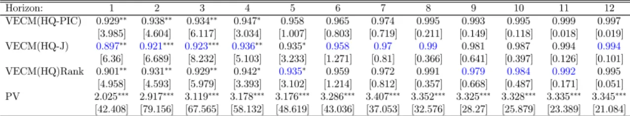
Table 10: Relative RMSFE of restricted models vs VAR for pt. Forecast period up

to 2007.

[3.985] [4.604] [6.117] [3.034] [1.007] [0.803] [0.719] [0.211] [0.149] [0.118] [0.018] [0.019] VECM(HQ-J) 0.897 0.921 0.923 0.936 0.935 0.958 0.97 0.99 0.981 0.987 0.994 0.994

[6.36] [6.689] [8.232] [5.103] [3.233] [1.271] [0.81] [0.366] [0.641] [0.397] [0.126] [0.101] VECM(HQ)Rank 0.901 0.931 0.929 0.942 0.935 0.959 0.972 0.991 0.979 0.984 0.992 0.995

[4.958] [4.593] [5.979] [3.393] [3.102] [1.214] [0.812] [0.357] [0.668] [0.487] [0.171] [0.051] PV 2.025 2.917 3.119 3.178 3.176 3.286 3.407 3.352 3.325 3.328 3.335 3.345

[42.408] [79.156] [67.565] [58.132] [48.619] [43.036] [37.053] [32.576] [28.27] [25.879] [23.389] [21.084]

See Notes of Table 2.

Table 11: Relative RMSFE of restricted models vs VAR for dt. Forecast period up

to 2007.

[2.433] [1.977] [1.995] [0.998] [0.761] [0.571] [0.718] [0.992] [0.908] [0.475] [0.338] [0.474] VECM(HQ-J) 0.952 0.873 0.806 0.826 0.928 0.958 0.965 0.941 0.917 0.937 0.939 0.93

[2.304] [5.904] [7.568] [5.988] [0.99] [0.477] [0.604] [2.013] [2.646] [1.434] [1.022] [1.026] VECM(HQ)Rank 0.964 0.94 0.812 0.825 0.919 0.945 0.955 0.934 0.912 0.929 0.938 0.934

[0.234] [0.002] [2.574] [4.742] [1.618] [0.755] [0.706] [2.188] [2.952] [1.762] [1.161] [1.022] PV 0.907 3.324 5.371 5.929 5.909 6.016 6.221 6.355 7.327 8.269 8.408 8.308

[1.742] [2.356] [5.903] [4.93] [9.502] [9.275] [10.018] [8.809] [9.065] [10.561] [10.227] [10.967]

Table 12: Relative RMSFE of restricted models vs VAR for pt. Forecast period up

to 2012.

[3.641] [2.255] [0.932] [1.489] [0.803] [0.1] [0.091] [0.103] [0.054] [0.003] [0.002] [0.025] VECM(HQ-J) 0.876 0.901 0.924 0.943 0.958 0.975 0.976 0.984 0.989 0.995 0.999 1.001

[5.729] [3.358] [4.425] [2.949] [1.599] [0.42] [0.322] [0.203] [0.553] [0.09] [0.001] [0.001] VECM(HQ)Rank 0.879 0.908 0.936 0.949 0.957 0.976 0.98 0.986 0.991 0.998 1.001 1.000

[6.201] [2.751] [2.425] [1.906] [1.369] [0.364] [0.145] [0.108] [0.449] [0.032] [0.004] [0.000] PV 2.001 2.834 3.044 3.104 3.14 3.204 3.212 3.19 2.948 3.027 3.037 3.051

[32.221] [81.764] [56.782] [48.517] [38.35] [36.047] [34.488] [33.279] [32.957] [33.91] [32.3] [37.36]

Table 13: Relative RMSFE of restricted models vs VAR for dt. Forecast period up

to 2012.

[0.069] [0.363] [0.387] [1.373] [0.212] [0.61] [1.491] [2.175] [2.097] [0.963] [0.157] [0.071] VECM(HQ-J) 0.921 0.889 0.826 0.809 0.869 0.86 0.851 0.841 0.928 0.96 0.977 0.976

[4.918] [2.804] [4.763] [4.612] [1.375] [1.124] [1.438] [2.494] [2.875] [1.666] [0.774] [0.641] VECM(HQ)Rank 0.933 0.976 0.865 0.807 0.844 0.848 0.859 0.852 0.924 0.952 0.974 0.973

[4.472] [0.679] [2.077] [3.544] [1.975] [1.899] [1.671] [2.515] [3.122] [1.942] [0.816] [0.823] PV 0.819 2.777 4.943 6.345 6.77 6.801 6.864 7.005 5.678 5.863 5.779 5.538

[7.448] [18.576] [24.418] [20.669] [14.578] [9.772] [8.519] [8.137] [7.423] [6.5] [5.757] [5.273]

(29)

and strategy (4, VECM(HQ)Rank). However, as is well known, econometric models are built to forecast mainly at shorter horizons, since, as the horizon increases, con-ditional forecasts converge to their unconcon-ditional counterparts. If we focus only on results at business-cycle horizons (1 through 5 years ahead), we have a clear winner strategy – strategy (3, VECM(HQ-J)) – which produces the best forecast model for 36.67% of occasions. The other two strategies, strategy (4, VECM(HQ)Rank) and PV model, produce the best models 26.67% and 25% of occasions, respectively.

Finally, we investigate if one of the 3 preferred methods – strategy (3, VECM(HQ-J)), strategy (4, VECM(HQ)Rank), and the PV model – produce forecasts that are statistically di¤erent from the others, employing the unconditional predictive ability test of Giacomini and White (2006). For ilr and isr, we …nd that strategy

(3, VECM(HQ-J)) have produced statistically better accuracy statistics than the PV model, while the converse is not true. Regarding the latter and strategy (4, VECM(HQ)Rank), there is no clear dominance, which also happens when we com-pared strategy (3, VECM(HQ-J)) and strategy (4, VECM(HQ)Rank). For Pt and

Dt, we …nd that strategy (3, VECM(HQ-J)) have produced statistically better

accu-racy statistics than the PV model and strategy (4, VECM(HQ)Rank), respectively, while the converse is not true. Forpt anddt, there is a clear pecking order as follows:

strategy (3, VECM(HQ-J)), strategy (4, VECM(HQ)Rank), and the PV model. All in all, if we have to recommend one forecast strategy for multivariate mod-els containing series subject to PVM restrictions, we would choose strategy (3, VECM(HQ-J)). Notice that it imposes cointegration restriction (theory) but esti-mates the cointegrating vector using econometric techniques.

5 Conclusion

This paper has two original contributions. The …rst is to show that PV relationships entail a weak-form SCCF restriction, as in Hecq et al. (2006) and in Athanasopou-los et al. (2011). It also implies a polynomial serial correlation common feature relationship (Cubadda and Hecq, 2001) for the VAR representation for yt and

(30)

dynamic system for these variables, something that has not been discussed before. Once we cast the PVM in these terms, it is straightforward to apply the toolkit of thecommon-feature literature for inference and testing.

Our second contribution relates to forecasting multivariate time series that are subject to PVM restrictions, which has a wide application in macroeconomics and …nance. We bene…t from previous work showing the bene…ts for forecasting when the short-run dynamics of the system is constrained for stationary data (Vahid and Issler, 2002), and when it is constrained for data subject to long- and short-run re-strictions (Issler and Vahid, 2001, Anderson and Vahid, 2011, and Athanasopoulos et al., 2011). The reason why appropriate common-cycle restrictions improve fore-casting is because it …nds linear combinations of the …rst di¤erences of the data that cannot be forecast by past information. This embeds natural exclusion restrictions preventing the estimation of useless parameters, which would otherwise contribute to the increase of forecast variance with no expected reduction in bias. The whole issue is obviously parsimony, but the exclusion restrictions are chosen in a way that is aligned with the …nal objective – to forecast the series in the system – eliminating parameters that go against that.

We applied the techniques discussed in this paper to data known to be subject to PV restrictions: the online series maintained and updated by Shiller at

(31)

References

[1] Anderson, H.M. and F. Vahid, (2011),“VARs, Cointegration and Common

Cycle Restrictions,” in “The Oxford Handbook of Economic Forecasting,” Edited by Michael P. Clements and David F. Hendry.

[2] Athanasopoulos, G., Guillen, O.T.C., Issler, J.V., and F. Vahid,

F. (2011), Model Selection, Estimation and Forecasting in VAR Models with

Short-run and Long-run Restrictions,Journal of Econometrics, Vol. 164(1), 116-129.

[3] Baillie, R. (1989), Econometric tests of rationality and market e¢ciency,

Econometric Reviews, 8, 151-186.

[4] Basistha, A., and Startz, R. (2008). Measuring the NAIRU with reduced

uncertainty: a multiple-indicator common-cycle approach. The Review of Eco-nomics and Statistics, 90(4), 805-811.

[5] Campbell, J.Y. (1987), Does Saving Anticipate Declining Labor Income?

An Alternative Test of the Permanent Income Hypothesis, Econometrica, vol. 55(6),1249-73.

[6] Campbell, J.Y. and R.J. Shiller (1987), Cointegration tests and present

value models,Journal of Political Economy 95, 1062-1088.

[7] Campbell, J.Y. and Shiller, R. (1988a). “The Dividend-Price Ratio and

Expectations of Future Dividends and Discount Factors” Review of Financial Studies, 58, pp. 495-514.

[8] Campbell, J.Y. and Shiller, R. (1988b).“Stock Prices, Earnings and

Ex-pected Dividends” Journal of Finance, 43, pp. 661-676.

[9] Campbell, J.Y. and A. Deaton (1989),Why is Consumption So Smooth?,

(32)

[10] Campbell, J.Y., Lo, A.W. and A.C. MacKinlay (1996),The Economet-rics of Financial Markets, Princeton University Press.

[11] Candelon, B. and Hecq, A.(2000),“Stability of Okun’s Law in a

Codepen-dent System,”Applied Economic Letters, 7, 687-693.

[12] Centoni, M., Cubadda, G. and A. Hecq (2007), Common Shocks,

Com-mon Dynamics and the International Business Cycle, Economic Modelling, vol.24, 1, 149-166.

[13] Chow, G., (1984), Econometrics. McGraw-Hill, New York.

[14] Cubadda, G. and A. Hecq (2001), On Non-Contemporaneous Short-Run

Comovements, Economics Letters, 73, 389-397.

[15] Engle, R.F. and C.W.J. Granger (1987), Co-integration and Error

Cor-rection: Representation, Estimation and Testing, Econometrica,55, 251-276.

[16] Engle, R.F. and S. Kozicki (1993), Testing for Common Features (with

comments), Journal of Business and Economic Statistics, 11, 369-395.

[17] Engle, R.F. and J.V. Issler (1995), Estimating Common Sectorial Cycles,

Journal of Monetary Economics, 35, 83-113.

[18] Engle, R.F. and Yoo, B. S. (1987), Forecasting and testing in co-integrated

systems. Journal of Econometrics, 35(1):143-159.

[19] Engsted, T. (2002),Measures of …t for rational expectations models.Journal

of Economic Surveys 16, 301-355.

[20] Giacomini, Raffaella and Halbert White, (2006),"Tests of Conditional

Predictive Ability,"Econometrica, vol. 74(6), pp. 1545-1578.

[21] Hamilton, J.D. (1994), Time Series Analysis (Princeton University Press:

(33)

[22] Hansen, L.P. (1982),Large Sample Properties of Generalized Method of Mo-ment Estimators,Econometrica, 50, 1029-1054.

[23] Hansen, Lars Peter and Sargent, Thomas J., (1981), "A note on

Wiener-Kolmogorov prediction formulas for rational expectations models," Eco-nomics Letters, vol. 8(3), pp. 255-260.

[24] Hansen, Lars Peter and Sargent, Thomas J., (1993), "Recursive

lin-ear models of dynamic economies," Proceedings, Federal Reserve Bank of San Francisco, March issue.

[25] Hecq, A., F. Palm and J.P. Urbain (2000), Permanent-Transitory

De-composition in VAR Models with Cointegration and Common Cycles, Oxford Bulletin of Economics and Statistics, 62, 511-532.

[26] Hecq, A., Palm, F.C., J.P. Urbain (2006), Testing for common cyclical

features in VAR models with cointegration, Journal of Econometrics, Volume 132(1), 117-141.

[27] Hecq, A., S. Laurent and F.C. Palm (2011), Pure portfolios models, RM

Maastricht University.

[28] Hoffman D.L and R.H. Rasche (1996),Assessing forecast performancee in

a cointegrated system,Journal of Applied Econometrics, 11, 495–517

[29] Issler, J.V. and F. Vahid. F. (2001), Common Cycles and the Importance

of Transitory Shocks to Macroeconomic Aggregates, Journal of Monetary Eco-nomics, vol. 47(3), pp. 449-475.

[30] Johansen, S. (1991), “Estimation and Hypothesis Testing of Cointegration

Vectors in Gaussian Vector Autoregressive Models,” Econometrica, vol. 59, pp. 1551-1580.

[31] Johansen, S. (1995), Likelihood-Based Inference in Cointegrated Vector

(34)

[32] Johansen, S. (2000), Modelling of cointegration in the vector autoregressive model, Economic Modelling, vol. 17, 359-373.

[33] Johansen, S. and A.R. Swensen (1999), Testing rational expectations in

vector autoregressive models, Journal of Econometrics, 93, 73–91.

[34] Johansen, S., and A. Swensen (2004), More on Testing Exact Rational

Expectations in Cointegrated Vector Autoregressive Models: Restricted Drift Terms, Econometrics Journal, volume 7, pp. 389–397.

[35] Johansen, S., and A. Swensen (2011),On a numerical and graphical

tech-nique for evaluating some models involving rational expectations, Journal of Time Series Econometrics, 2011, vol. 3, issue 1.

[36] Keane, Michael P. (2010), “Structural vs. atheoretic approaches to

econo-metrics,”Journal of Econometrics, Vol. 156 (1), pp. 3–20.

[37] Patton, A., Tarun Ramadorai and Michael Streatfield (2013),

“Change You Can Believe In? Hedge Fund Data Revisions,” Working paper: Duke University.

[38] Reinsel, G.C. and S.K. Ahn (1992), Vector Autoregressive Models with

Unit Roots and Reduced Rank Structure: Estimation, Likelihood Ratio Tests, and Forecasting, Journal of Time Series Analysis, 13, 353-375.

[39] Vahid, F. and R.F. Engle (1993), Common Trends and Common Cycles,

Journal of Applied Econometrics, 8, 341-360.

[40] Vahid, F. and R.F. Engle (1997), Codependent Cycles, Journal of

Econo-metrics, 80, 199-221.

[41] Vahid, F., J.V. Issler (2002), The importance of common cyclical features

(35)

A

Appendix: Testing present-value models with

a common-cycle approach

The discussion of this paper suggests that, for integrated Yt and yt, there are three

di¤erent instances in which we can investigate the validity of PVMs. First, the cointegration test for Yt and yt, if both are I(1). Second, the (invariant) rank

restrictions in the VECM or the transformed VAR. Third, the coe¢cient restrictions and unpredictability properties for linear combinations. In order to test for PVMs, we propose the following steps:

1. Choose consistently the order of theV AR(p)for the jointI(1)process (Yt; yt)0

using di¤erent information criteria.

2. Given our choice ofp;test for the existence of cointegration betweenYt and yt.

If that is the case (there exists one cointegrating vector), estimate the long-run coe¢cient , in St = Yt yt, super-consistently using the likelihood-based

trace test proposed by Johansen (1995). Alternatively, the Engle and Granger (1987) regression test can be carried out. In either case, formS^t=Yt ^yt. If

there is no cointegration, the PVM is rejected.

3. Given p and S^t; test for the weak form common feature using a reduced rank

test for( Yt; yt)0. We can use both a likelihood ratio multivariate approaches

(e.g. a canonical correlation analysis) and a single-equation approach (e.g. GMM). Because most present-value relationships apply to heteroskedastic …-nancial data, one may prefer a GMM framework on the basis that it easily embeds robust variance-covariance matrices for parameters estimates. Indeed the canonical correlation approach assumesi:i:d:disturbances.

(36)

4. Integrate steps 2 and 3, estimating jointly long-run and short-run parameters as in Centoni, Cubadda and Hecq (2007).

Integrate steps 1, 2 and 3, estimating jointly the lag length of the VAR and long-run and short-run parameters as in Athanasopouloset al. (2011).

A.1 LR tests for i.i.d. disturbances

The canonical-correlation approach entails the use of a likelihood ratio (reduced-rank regression) test for the weak-form common features in the V ECM(p 1) for

( Yt; yt)0. It can be undertaken using the canonical-correlation test on zero

eigen-values, which are computed from:

CanCor 8 > > > > > > > > > > < > > > > > > > > > > : Yt yt ! ; 0 B B B B B B B B B B @

Yt 1

.. .

Yt p+1

yt 1

.. .

yt p+1

1 C C C C C C C C C C A

j(Dt;S^t 1)

9 > > > > > > > > > > = > > > > > > > > > > ; ; (38)

where CanCorfXt; WtjGtg denotes the computation of canonical correlations

be-tween the two sets of variables Xt and Wt; concentrating out the e¤ect of Gt

(de-terministic terms and a disequilibrium error-correction term) by multivariate least squares. The previous program (38) is numerically equivalent to

CanCor 8 > > > > > > > > > > > > < > > > > > > > > > > > > : 0 B @ Yt yt ^

St 1

1 C A; 0 B B B B B B B B B B B B @

Yt 1

.. .

Yt p+1

yt 1

.. .

yt p+1

^

St 1

1 C C C C C C C C C C C C A

jDt

(37)

which is more convenient to directly obtain the coe¢cient of S^t 1 in (10). The

likelihood ratio test, denoted by _LR;considers the null hypothesis that there exist at leastscommon feature vectors. It is obtained in LR = T

s

P

i=1

ln(1 ^i); s= 1;2;

where ^i are the i-th smallest squared canonical correlations computed from (38)

or (39) above, namely from ^_XX1 ^XW^W W1 ^W X; or similarly from the symmetric

matrix ^_XX1=2^XW^_{W W}1 ^W X^_XX1=2; where ^ij are the empirical covariance matrices,

i; j =X; W.

In the bivariate case, the unrestricted VECM has4(p 1)+2parameters, whereas the restricted model has2(p 1) + 2 + 1. The number of restrictions when testing the hypothesis that there exists one WF common feature is then2(p 1) 1 = 2p 3

forp >1:7 _{As proposed in Issler and Vahid (2001), we can obtain the same statistics}

by computing twice the di¤erence between the log-likelihood in the unrestricted

V ECM(p 1)for( Yt; yt)0and in the pseudo-structural form estimated by FIML:

1 0 0 1 ! Yt yt !

= _~0

1

Yt 1

yt 1

!

+:::

+ _~0 p 1

Yt p+1

yt p+1

!

+ ( 1 0 2) ~2

St 1+

v1t

v2t

:

For the transformed VAR the restriction underlying the restricted PSCCF can be tested using: CanCor 8 > > > > > > > > > > > > < > > > > > > > > > > > > : 0 B @ ^ St yt ^

St 1

1 C A; 0 B B B B B B B B B B B B @ ^

St 1

^

St 2

...

^

St p

yt 2

...

yt p+1

1 C C C C C C C C C C C C A

jDt

9 > > > > > > > > > > > > = > > > > > > > > > > > > ; ;

7_{In the VECM, the general formula for} _n _{series that can be annihilated by}_s _{combinations is}

(38)

where the number of parameters in the unrestricted model is4(p 1)+2;the restricted model has 6 + 2(p 2); the number of restrictions is 2p 4 in case of unrestricted

~₁:

1 ~0

0 1

!

St

yt

!

= ~_~1a

1b

St 1

yt 1

!

+:::

+ _~0 p 1

St p+1

yt p+1

!

+ 0 0

~_p;p ₀

!

St p

yt p

!

+ u1t

u2t

:

If ~₁ is restricted we have 2p 3 restrictions and the pseudo structural form is

1 ~₀

0 1

!

St

yt

!

= #1 0

~₂_;₁ ~₂_;₂

!

St 1

yt 1

!

+

0 ~_p ₁

St 2

yt 2

!

+ + _~0 0

p;p 0

!

St p

yt p

!

+ u1t

u2t

:

Notice that this set of rank restrictions are identical to the ones in Campbell and Shiller (1987) if one imposes zero restrictions in the last matrix coe¢cient in their setup8_{. The proposed approach to testing PVMs here is to …rst test the rank}

condi-tion (necessary) without imposing yet any further parameter restriccondi-tions. As argued above, the rank condition is invariant to how we write the PV equation linking Yt

and yt. If not rejected, then we can test the additional restrictions on matrices

co-e¢cients, which are not invariant to how we write the PV equation. Putting more weight on invariant restrictions satis…es robustness, since, not only a di¤erent de…n-ition of the timing ofYt and/oryt, but also the presence of measurement error, data

revisions, all will lead to the correct rank condition to be met but imply di¤erent parameter values in the di¤erence equation generating PVMs. An additional reason to follow this path is that we will be able to split both e¤ects, shedding light on the exact reason for rejecting theory if that is the case. Understanding why we reject a given PVM is an important issue, since di¤erent authors have complained that

(39)

cross-equation restriction tests reject PVMs too often, even in cases where theory is …rmly believed to hold and that graphical analysis seems to support that view.

A.2 Regression-Based GMM Tests

Testing with a GMM approach entails testing the common feature null hypothesis using an orthogonality condition between a combination of variables in the model

Yt; yt;S^t 1

0

and the conditioning set W0

t. For example, in the context of (8),

we would have the following moment restrictions:

E([ Yt 1 yt 2S^t 1] W

0

t) = 0; (40)

where we would have additionally to test H0: 1 = 0 and 2 = 1 using a Wald

test. Prior to that, we want to estimate 1 and 2 and test the validity of the

over-identifying restrictions in (40). The use of IV type estimators and the associated orthogonality tests is straightforward in this context. Let us considerWt the vector

of instruments de…ned as before (an intercept is added). The GIVE estimator is simply the 2SLS or the IV estimator when the instruments are the past of the series, namely

^_{GIV E} ₌ _X0

W(W0W) 1W0

X 1 X0

W(W0W) 1W0

Y ; (41)

with X_t= ( yt;S^t 1;1)0: The validity of the orthogonality condition and

conse-quently the presence of a common feature vector is obtained via an overidenti…cation J-test (Hansen, 1982)J1( ) =T gT( ;:)0P_T1gT( ;:);whose empirical counterpart is:

J1( IV) = (u 0 _~

W)(^2_uW~0 _~

W) 1(W~0 u):

The variance-covariance matrix of the orthogonality condition has under usual reg-ularity properties the sample counterpart P^T = (1=T)^2u(W~

0 ~

W) with ut = Yt

^₁ yt ^2S^t 1. W~ is the demeanedW;namelyW~ =W i(i

0

i) 1iW(withi= (1:::1)0 )

(40)

the constant vector.

All the estimates and tests presented above embedded the assumption of ho-moskedasticity. This may be …ne for macroeconomic data, such as consumption and income, but is clearly at odds with …nancial data. Candelonet al. (2005) have illus-trated in a Monte Carlo exercise that LR has large size distortions in the presence

of GARCH disturbances. We implement the GIVE estimator by using the White’s HCSE estimator such that (see Hamilton, 1994):

^_{GM M} ₌ _X0

W(W0BW) 1W0

X 1 X0

W(W0BW) 1W0

Y ; (42)

where the only di¤erence between^GM M and the usual^GIV Eis the presence of an

ad-ditional diagonal matrixB=diag(u2

1; u22; :::u2T)whereut = Yt ^1IV yt ^2IVS^t 1

are the residuals obtained under homoskedasticity using the GIVE estimation in a …rst step. For testing, we form the following new sequence of residuals u_t =

Yt ^1GM M yt ^2GM MS^t 1;and use these to compute a new J-test robust to

heteroskedasticity:

J2( GM M) = (u 0W~ )(W~ 0B ~W) 1(W~ 0u ): (43)

Note that alternative approaches have been evaluated in Hecq an Issler (2012).

A.3 Small sample properties of PVM tests

A small Monte Carlo simulation might help to advise the use of one of the tests considered. We use T = 100 observations with 10;000 replications. The lag length of the VAR in level in the data generating process is chosen to be p = 3: However, we estimate the model forp= 2;3 and 5. The DGP that ensures 0

= (1 : 0) is:

Yt

yt

!

= 0:05 0:05

!

+ 0 0

0:5 0:2

!

Yt 1

yt 1

!

+:: 0 0

0:4 0:2

!

Yt 2

yt 2

!

+ 1

0:75

!

1 ₁ Yt 1

yt 1

!

+ u1t

u2t

!

(41)

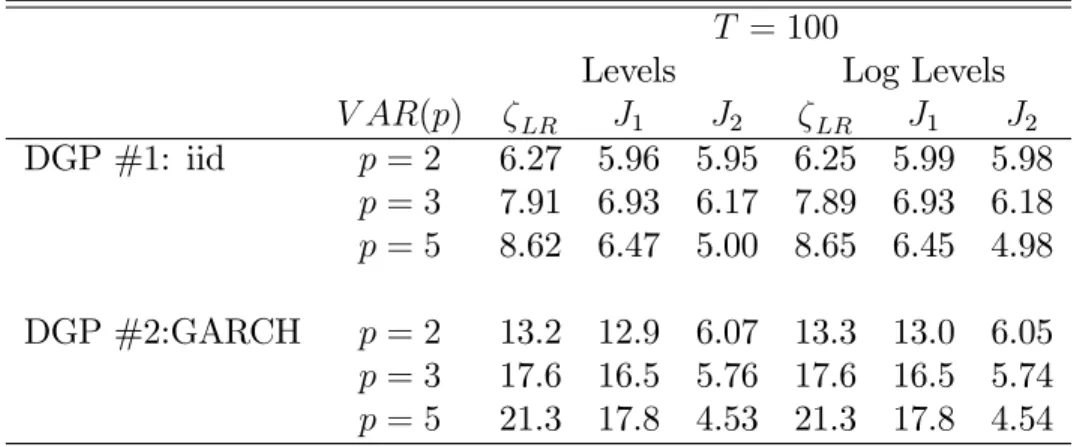
Table 14: Empirical size (nominal set to 5statistic

T = 100

Levels Log Levels

V AR(p) _LR J1 J2 LR J1 J2

DGP #1: iid p= 2 6.27 5.96 5.95 6.25 5.99 5.98

p= 3 7.91 6.93 6.17 7.89 6.93 6.18

p= 5 8.62 6.47 5.00 8.65 6.45 4.98 DGP #2:GARCH p= 2 13.2 12.9 6.07 13.3 13.0 6.05

p= 3 17.6 16.5 5.76 17.6 16.5 5.74

p= 5 21.3 17.8 4.53 21.3 17.8 4.54

We considered two types of error terms for the VECM above: in the …rst DGP, labelled DGP # 1 in Table13, the disturbance term is bivariate normal with a unit variance and a correlation of 0:5;in the second process, labelled DGP # 2, the dis-turbance terms are governed by a bivariate GARCH process (CCC) with a yesterday news coe¢cient of 0:25, a coe¢cient of persistence of 0:74, and a long run variance equals 0:01. Note that yesterday’s news coe¢cient is larger than what is usually found empirically (between 0:10 and 0:15). The theoretical coe¢cients in the rela-tionship Yt= 1 yt+ 2St 1+ut are 1 = 0 and 2 = 1 :Here, for simplicity,

we set ₁ = 1 in the DGP but the cointegrating vectorYt ^yt is estimated using

Johansen’s approach.

Table 13 reports the empirical rejection frequency at the 5% signi…cance level (nominal size). In the iid case, the behavior of the tests is rather similar. Results get much more worse in the presence of time varying conditional variances. With heteroskedastic data, the robust-White GMM test has proper size.

In the last three columns of Table 14 we report the rejection frequencies of the same three tests applied to the logarithms of the variablesYtandytbut for the same