Common factors in Latin America's business cycles

(1)

•

• _•

•

,.

,

• SEMINARIOS DE ALMOÇO

•

FUNDAÇÃO

DA EPGE

•

GETUUO VARGAS

•

• Common factors in Latin America's

• business cycles

•

• _•

• LUIS CATÃO

•

• (lGIER, Bocconi University)

• _•

•

• _•

Data: 19/08/2005 (Sexta-feira)

•

• Horário: 12 h 15 min

•

• _•

Ｌｾ＠

Local:

•

Praia de Botafogo, 190 - 11 o andar

• FGV

Auditório nO 1

•

, EPGE

Coordenação:

•

Prof. Luis Henrique B. Braido

•

e-mail: [email protected]

•

• _•

(2)

•

• _•

•

• S

5

•

• _•

5

•

• _•

•

• _•

•

• _•

•

• _•

•

• _•

Common Factors in Latin America's Business Cycles

Marco Aiolfi

a ,

Luis

ｃ｡ｴ￣ｯ｢ｾ＠

Allan Timmermann

c

aIGIER, Bocconi University

bResearch Department, International Monetary F\md

CUC San Diego This Draft: 15 August 2005

Abstract

This paper constructs new business cycle indices for Argentina, Brazil, Chile, and Mexico based on common dynamic factors extracted from a comprehensive set of sectoral output, external trade, fiscal and financial variables. The analysis spans the 135 years since the insertion of these economies into the global econ-omy in the 1870s. The constructed indices are used to derive a business cyc1e chronology for these countries and characterize a set of new stylized facts. In particular, we show that ali four countries have historically displayed a striking combination of high business cyc1e volatility and persistence relative to advanced country benchmarks. Volatility changed considerably over time, however, being very high during early formative decades through the Great Depression, and again during the 1970s and ear1y 1980s, before declining sharply in three of the four countries. We also identify a sizeable common factor across the four economies which variance decompositions ascribe mostly to foreign interest rates and shocks to commodity terms of trade.

Keywords: Business Cyc1es, Factor Models, Latin America

JEL classification: E32, N10

(3)

1 Introduction

Wbat gives rise to the business cycle and how it evolves over time is a key question in

macroeconomics. Since business cycle volatility can arise from various sources and be

exacerbated by clistinct economic policy regimes, slowly-evolving institutional factors

(Acemoglu et alo 2(03) and degrees of financial and trade openness (Kose et al. 2(05),

a better understanding of it requires taking a long view at the phenomenon so as to

cover a range of distinct policy and trade regimes and institutional settings. Yet there is

a striking dearth of systematic work along these lines for most countries outside North America and Western Europe.

One region that is particularly under-researched is Latin America. This gap is

somewhat surprisiing not on1y because the region is deemed as highly volatile and the

question of what drives such volatility is of interest in its own right; it is also surprising because the region comprises a large set of sovereign nations which have gone through a number of dramatic changes in policy regimes and institutions over a long period

of time and re1ative to other developing countries in Africa and Asia (many of which

only became independent nations in recent decades), thus providing a rich context for assessing business cyc1e theories. Indeed, Latin America is notoriously absent in the well-lmown historica1 business cycle studies by Sheffrin (1988) and Backus and Kehoe

(1992), and on1y Argentina is covered in more recent work along similar lines

(Basu

and Taylor, 1999). Instead, recent research on Latin American business cyc1es has been either country-specific and covered only short periods of time (e.g. Kydland and Zarazaga, 1997) or focused on specific transmission mechanisms and limited to post-1980 data (Hoffmaister and Roldai, 1997; Neumeyer and Perri, 2005).1 A coro11ary of this gap in the litR..rature is the absence of any formal attempt to establish a reference cyc1e dating for these countries similar to those available for others-such as the United

States and the Euro area-on the basis of a variety of coincident and leading indicators

(Moore, 1983; Gordon, 1986; Artis et al., 1997; Stock and Watson, 1999).

This paper seeks to fill some of this lacuna. Unlike previous work, we go back as

1 A notable exception is Engle and Issler (1993) who use a multivariate version of the

Beveridge-Nelson trend-cycle decomposition to test for the existence of common trends and common cycles in the real GDP of Argentina, Brazil, and Mexico during 1948-86. They do not provide evidence, however, of what drives the common regional cycle they extract, Dor do they look at key variables such as terms of trade or fiscal and monetary shocks that might help explain the observed country-specific movements. Furthermore, their analysis is entirely univariate and is conducted at the country leveI.

2

• _•

•

• _•

•

• _•

•

• _•

•

• _•

•

• _•

•

• _•

•

• _•

•

(4)

•

• _•

•

• _•

•

• _•

•

• _•

•

• _•

•

• _•

•

• _•

•

• _•

•

• _•

•

far as available macroeconomic data permits and jointly focus on fOUI of the largest Latin American economies - Argentina, Brazil, Chile, and Mexi.co. Together, these countries have accounted for some 70 percent of the region's GDP over the past half century (Maddison, 2003, pp.134-140) , thus clearly setting the tone for the region's overall macroeconomic performance. At the same time, data availability for this subset of countries permits us to provide a long-run cbaracterization of the business cycle in these economies similar to that conducted for advanced countries.

The construction of new indices of economic activity and the identification of

volatil-ity SOUICes over such long period allows us to address fOUI main questions. First, how

volatile has Latin America been relative to other countries? In particular, has economic

activity in Latin America been more or less stable in periods of greater trade and

finan-cial integration with the world economy, such as during the pre-1930 gold standard and

the post-1980 period? Second, has this volatility been the result of sma1l and frequent

shocks, giving rise to smooth patterns of output ftuctuations around trend, or has it been dominated by large and infrequent but persistent shocks? Third, do we observe

similar stylized facts as those documented for other economies that feature in the

ex-isting business cycle literature? Finally, is there an identifiable regional business cycle

and, if so, what drives it?

As discussed further below, a key requirement for answering these questions is to

obtain a measure of economic activity that is expected to be reasonably accurate and

consistent over such a long period. We provide this by constructing a new index of eccr nomic activity for each of the fOUI countries using a dynamic common factor methodol-ogy which, to the best to OUI knowledge, is for the first time applied to build a business cycle index for this set of countries. This methodology is applied to a uniquely large set of macroeconomic variables compiled from a wide range of historical SOUIces. The data span key sectors such as agricultura!, manufacturing, mining and cement production,

fiscal expenditUIes and revenues,

externaI

variables such as terms of trade, the real

exchange rate and import and export volume, as well as a host of financiaI indicators

including interest rates and monetary aggregates.

Our

index of economic activity is

shown to track very closely the existing real GDP data from the full set of national

of economic activity is constructed as the common factor that underlies a wide set of macroeconomic and sectorial indicators - thus filtering out idiosyncratic components

(5)

(including possible measurement errors) - it provides a measure that is germane to the

very concept of the business cycle as defined in the work of Burns and Mitchell (1946)

- which still forms the backbone of the widely used NBER reference cycle indicator for

the United States.

The paper's main findings are as follows. Over the full sample ＱＸＷｾＲＰＰＴＬ＠ the

average business cycle volatility in ali four countries has been considerably higher than

in the advanced eeonomies-albeit with important differences over sub-periods. Latin

American ｶｯｬ｡ｴｩｬｩｾ＠ was highest in the pre-1930 era, during the formative years of key

national institutioDS. It then dropped sharply during the four decades following the Great Depression - an apparent significant pay-off of the inward-looking growth and highly interventionist policy regimes at a time when volatility in advanced countries rose to ali-time highs. Cyclical instability in Latin America bounced back again in the

1970s and 1980s - when it was more than twice as high as the advanced country average

- before declining sharply more recently to unprecedented low levels. Throughout the

period, cyclical persistence has been high, with large shocks giving rise to a striking

combination of high cyclical volatility and long business cycle durations relative to advanced country standards.

We also find evidence of a number of regularities high1ighted in the existing business

cycle literature. In particular, external terms of trade have been strongly procyclical,

the trade balance counter-cyclical, and fixed investment has been several times more

volatile than output. Using the simple gauge proposed in Karninsky,

Reinhart,

and

Végh (2004), we also find that fiscal policy has been strongly procyclical in these

coun-tries. In contrast with evidence more directly supportive of Phillips curve trade-offs

among advanced rountries, we find that inHation has been historically counter-cyclical in ali four Latin American economies. Compared with the more mixed cross-country

evidence in other regions, real wages have also been broadly procyclical. Once again,

a main contrast with advanced economies lies in the strikingly large volatility of these individual variables.

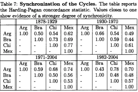
Concordance indices along the lines of Artis et al (1997) and Harding and Pagan

(2002) indicate that business cycles in these economies have been reasonably correlated.

This raises the question of whether there has been a common Latin American business

cycle and, if 80, what drives it? Pooling data from ali four countries, the common

factor methodology we employ permits the identification of a common regional factor.

4

•

• _•

•

• _•

•

• _•

•

• _•

•

• _•

•

• _•

•

• _•

•

• _•

•

(6)

•

• _•

•

_ｾ＠

s

•

• _•

•

• _•

•

• _•

•

• _•

•

• _•

•

• _•

•

• _•

This provides the basis for a more robust test of the hypothesis that global shocks

(notably shocks to key foreign interest rates such as UK and US Treasury bond rates) have been important in driving capital flows and business cyeles in Latin America

-an issue with salient practical implications that has previously been addressed using

more restrictive empirical approaches and limited data (Calvo et alo 1993;

Fernandez-Arias, 1994; Agénor et al., 2000; Neumeyer and Perri, 2(05). Using a VAR framework

that also allows for the roles of world primary commodity terms of trade and foreign

output shocks and using generalized variance decompositions, we show that shocks to

global interest rates, terms of trade, and foreign output account for between 40 to 70

percent of forecast error variance in the regional common component across the various sub-periods and policy regimes.

The remainder of the paper is divided into four sections as follows. Section 2 lays

out the econometric framework and discusses the main estimation issues. Section 3

provides a brief description of the variables and presents initiaI estimates. Section 4 places our results in an economic context and presents a business cyele chronology for the four countries. Section 5 examines the extent of regional co-movements and the role of common shocks. Section 6 coneludes.

2 Econometric FraIllework

The idea that a cross-section of economic variables share a common factor structure has

a long tradition in economics, dating back at least to the attempt by Burns and Mitchell

(1946) to construct an aggregate measure of economic activity. There are two chief motivations for common factor models. One is that economic theory suggests strong linkages between economic activityacross different sectors due to common productivity, preference, policy shocks but since some of these shocks unobservable, information

about them can only be extracted once one has access to a sufliciently large

cross-section of economic variables that are at least in part driven by these shocks. Hence, a

critical requirement that needs to be met in our analysis is the availability of broad and a

diverse enough set of variables that bear sufliciently elose relation to aggregate business cyele behavior. Natural candidates inelude capital formation, government revenue and

expenditures, sectorial output series, as well as a externaI trade figures and a host of

financiaI variables. The fact that the Latin American economies have historically been

(7)

highly dependent on global capital markets and demand from outside trading partners suggests that interest rates and cyclical output in advanced countries also be included in the analysis.

The second motivation for using dynamic factor analysis is related to the presence of measurement erroIS. Activity leveis in many sectors are measured with considerable error. Provided that measurement errors are largely idiosyncratic, cross-sectional in-formation can be used to construct more robust common factors that are not similarly sensitive to the impact of such errors. Here one has to make assumptions on the

expo-sure of such ohservable variables to common shocks in order to identify the underlying

driving factors.

Stock and Watson (1989, 2002) and Forni, Hallin, Lippi and Reichlin (2000) have shown that the application of dynamic common factor models to a suflicient1y rep-resentative set of macroeconomic and sectorial indicator provides superior forecasting

performance for a target variable such as real GDP or indeed any broad index of

eco-nomic activity. This methodology turns out to be particularly useful when some of the

constituent series that add up to a target variable (such as monthly GDP) are

lack-ing, or when such series are suspected to be mismeasured (as commonly deemed to be

the case for certain service activities). An important requirement is that such

mea-surement errors are sufficiently idiosyncratic or that the cross-section of available time series be sufficiently large and/or representative. This methodology is clearly suitable when interest lies in reconstructing (backcasting) historical measures of the cycle.

2.1 Dynamic

Factor Models

In the following we explain how information on the unohserved factors can be extracted.

Let Xt be a vector of de-meaned time series ohservations on N economic variables

observed over the sample t = 1, ... , T. Assllroing that X admits a dynamic factor

representation we can write

(1)

(2)

6

• _•

•

• _•

•

• _•

•

• _•

•

• _•

•

• _•

•

• _•

•

• _•

•

• _•

•

(8)

•

• _•

••

•

5

•

6

•

• _•

•

• _•

•

• _•

•

• _•

•

• _•

•

• _•

•

• _•

where ft

=

(llt,

... ,

fqt)' is a vector of

q

common dynamic factors, A (L) is an

Nxq

matrix

of filters of length s, ｾ＠ is an N x 1 vector of idiosyncratic disturbances, F t =

(r;, ... ,

fLs)

is an r x 1 vector of stacked factors with r = q x (s

+

1). Notice that while q identifies the

number of common shocks, the dimension of F t

(r)

dependa on the lag structure of the

propagation mechanjsm of those shocks. We refer to (1) as the dynamic representation

and to (2) as the static representation. Similarly, ft is the vector of q dynamic factors

and Ft the vector of r static factors, while the

A

matrices contain the factor loadings.

In practice the factors are typically unobserved and extraction of them from the

observables (Xt ) requires making identifying econometric assumptions. It is common

to assume that the errors, ｾＬ＠ are mutually orthogonal with respect to ft although

they can be correlated across series and through time. In addition the factors are only

identified up to an arbitrary rotation-we explain in the empirical section how we choose a particular rotation using the idea that the factors are only identified indirectly via the factor loadings.

When applied to a broad cross-section of economic variables, this model is ideally suited to extract information on common components of economic activity. The extent

to which information in the q common factors provides a broad-based measure of ･｣ｾ＠

nomic activity dependa crucially on the quality and representativeness of the underlying

economic variables, 50 successful implementation of the approach must be preceded by

careful construction of a data base comprising information on sectorial output variables,

govemment activity, external trade, financiaI variables and 50 forth.

2.2 Factor Estimation

The standard estimation method of dynamic factor models involves maximizing the

likelihood function by means of the Kalman filter. This technique has been employed

for low-dimensional systems by Stock and Watson (1991) and for higher dimensional systems (N=60) where the maximization is undertaken using the EM algorithm. When

N is large, non-parametric methods such as static principal components (Stock and

Watson (2002)), weighted static principal components (Boivin and Ng (2003)) and dynamic generalized principal components (Forni, Hallin, Lippi and Reichlin (2000)) are available for consistent estimation of the factors in approximate dynamic factor models.

(9)

Under the assumed orthogonality between the dynamic factors and the idiosyncratic

disturbances, we c.an consider a spectral density matrix or covariance matrix of the X_t

decomposition and the common component can be approximated by projecting either

on the first r static principal components of the covariance matrix (Stock and Watson,

2002) or the first q dynamic principal components (Forni, Hallin Lippi and Reichlin,

2000), possibly after scaling the data by the covariance matrix (Boivin and Ng (2003)).

In the following we briefly deserihe these approaches.

Stock and Watson (2002) proposed a principal component estimator of the factors as the solution to the following least squares problem:

subject to the restriction A'A = I. The solution to this problem takes the form

(3)

where v is an r x 1 vector of eigenvectors corresponding to the r largest eigenvalues of

the variance-covariance matrix of the X-variables,

:E

xx . The resulting estimator of the

factors,

FF,

is the fi.rst r static principal components of Xt .

Forni et al (2000) exploit dynamic structure in the factors by extracting principal components from the frequency domain. Their approach permits efticient aggregation of

variables that may be out of phase. In this case the common componen.t is estimated by

projecting the X-variables on present, past and future dynamic principal components. The factors and their loadings are the solution to the following non-linear least squares

problem that weights the idiosyncratic errors by their variance covariance matrix,

n

=

E[(Xt - AFt ) (Xt -

AFd):

again subject to A' A

= I. Forni et al (2oo3b) consider a two-step weighted principal

components analysis where they estimate n as the difference between the sample

co-8

• _•

•

• _•

•

• _•

•

• _•

•

• _•

•

• _•

•

• _•

•

• _•

•

• _•

•

(10)

•

• _•

•

6

•

• _•

_.,

• _•

•

• _•

•

• _•

•

• _•

•

• _•

•

ｾ＠

variance matrix, Exx, and the dynamic principal components estimator of the spectral

density matrix of the common components.2

The resulting estimators of the loadings and common factors are

ｾ＠

A - vg

FfHLR

-

ｾｘｴ＠ =

v'X

t ,

(4)

where vg are the generallzed eigenvectors associated with the largest generalized

eigen-values of the estimated covariance matrices of common and idiosyncratic components

and the resulting estimator of the factors is the vector consisting of the first r

gen-erallzed principal components of Xt . This can be seen a the first r static principal

components of the transformed data

X

t =

(fi)

-1/'2 Xt . An advantage of this approach

is that it exploits the dynamic structure in the variance covariance matrix of the data, accounting for leading or lagging relationships among variables which can be out of

phase by deriving an estimate of

n

through dynamic principal components methods.3

An important requirement when applying these estimators is that all the variables

entering the dynamic common factor specification are stationary. With the exception of

the inflation rate, real interest rates, and the ratios of export to import value which are

stationary by construction, we employ two alternative approaches to ensure stationarity.

One is the standard Hodrick-Prescott filter, with the smoothing factor

(À)

set to 100,

as is common practice with annual data (c.f. Backus and Kehoe, 1992). The second

approach to detrending considered here is the symmetric moving average band-pass

filter advanced by

Baxter

and King (1999). Following common practice with annual

data, we set the size of the symmetric moving average parameter K=3 but use a

larger-2Specifically, let Xt denote the standardized values of Xt . The estimated spectrum of Xt, Szz(w),

is computed at 101 equally spaced ordinates using a Bartlett kernel applied to p = Tl/2 sample

autocovariances. The estimated spectrum ofthe dynamic factor components, SJf(w), is computed for each of the 101 frequencies using q dynamic principal components of Szz(w). The estimated value of

n

is computed as n = Ezz - Eff' where Ezz is the sample second moment matrix of x and EIf is the inverse fourier transform of Sff(w).

31n their empirical forecasting comparison D'Agostino and Giannone (2004) find that weighted procedures generally produce better forecasting performance. Similarly, Boivin and Ng (2003) find that weighted principal components improve on the forecasts of the standard principal components methods applied to the static factor model. Stock and Watson (2005) report that forecasts based

on factors estimated with static principal components and those estimated with weighted principal components tend to be high1y correlated.

(11)

than-usual bandwidth ranging from 2 to 20 years so as to avoid filtering out the longer

(12-20 year)

pre-war cycles first documented by Kuznets

(1956)

for the United States

and found to be present in severa! advanced countries (Solomou,

1987). As

shown below,

both detrending methods yield very similar results. Finally, since we are concemed with

a real economic aggregate, all variables are measured in real terms (deflated by the

consumer price index or by the GDP deflator) with the obvious exceptions of inflation,

the ratios of exports to imports, and country spreads (as measured by the difference

between the yield on a sovereign foreign-currency denominated bond and the respective

UK or US yields). We employ the commonly used of defining the real interest rate as

the difference between the nominal interest rate and current inflation. Since all interest

rate series used in the estimation refer to short-term instruments, discrepancies arising

from possible mismatches between current and expected inflation are les.s criticaI than

in the case of long bonds.4

2.3 Backcasting Historical Activity Measures with Dynamic

Factors Model

The common factors derived above,

Frv

or

Ff

H LR, are of interest in their own right

since they provide broad-based measures of economic activity. However, often particular

interest lies in ana1yzing a particular time-series such as GDP growth over long periods

of time. This immediately poses two problems. First, data on this variable may only

be available over a more recent sample. Second, even when available, the series may be subject to considerable measurement error.

The common factor approach is ideally suited to handle these problema provided

that the variable of interest lends itself to a similar dynamic factor representation as

assumed above. In particular, let GDP growth be represented by the variable Yt. Under

the assumption that Yt is driven by the common factors ft =

(flt, ... ,

fqt)' derived above,

we have

(5)

Our interest lies in. backcasting values to create a new historicaI time-series of output

growth so we estimate the following backcasting equation using contemporaneous factor

4We also checked the robustness of our results to the use of the US 10-year bond yield and found that this did not have any effect on inferences made in the paper.

10

•

• _•

•

• _•

•

• _•

•

• _•

•

• _•

•

• _•

•

• _•

•

• _•

•

• _•

(12)

•

• _•

•

• _•

•

• .,

•

• _•

•

• _•

•

• _•

•

• _•

•

• _•

•

• _•

•

values:

Yt =

a

+

f3'F

t

+

Et·

Data of sufficient quality on Yt is only available over a much shorter (recent) sample

than data on the variables used to construct estimates of the factors. However, under

the maintained mode! (5), we can estimate the parameters () =

{a,,B}

over a (recent)

sample period for which quality data is available on output growth, y. We can then

backcast output growth over the longer sample for which estimates of the factors are

available. In the following we explain details of how we set up the data and implement

these ideas .

3 Reconstructing Broad Measures of Economic

Ac-tivity in Latin America

A full set of national income account data for Argentina, Brazil, Chile and Mexi.co is onlyavailable from the mid-1930s (Argentina) or starting at some point in the 1940s for

the other three countries.5 _{Previous researchers have tried to overcome this limitation}

by constructing proxy measures of economic activity for the earlier period. The quality

of these constructs is, however, very uneven due to the lack and/or the very poor

quality of output data for broad sectors of the economy. In the case of Argentina and

Brazil, for instance, offi.cial output data in agriculture, manufacturing, construction, and services only become available from 1900 onwards and, even then, with serious gaps particularly in the case of Brazil (c.f. Haddad, 1978). With regard to Chile and

Mexico, sectorial output data stretching back to the 19th century are more readily

available but, again, often spanning a small subset of the universe of firms and of

questionable quality (see the Appendix). Insofar as previous researchers tried to derive an aggregate measure of economic activity from averages of these production data

(resorting to linear interpolation to fill gaps in some discontinuous annual series), the

resulting indices are bound to be highly inaccurate. While two other attempts have

been made to overcome these problems, they have clear drawbacks. One is that of

5Even for Argentina, full-fledged information underpinning national account estimates is not avail-able before 1950 (see Banco Central de Argentina, 1976). In the case of Mexico, a GDP series con-structed solely on the basis of sectoral output information-and not based on expenditure and income data-has been reported by Banco de Mexico since 1921.

(13)

backcasting Argentine GDP based on a handful of production and trade variables by means of linear OL8 regressioDS (della Paolera, 1988, p.189)j the other is the use of static common components to backcast 19th century Brazilian GDP on the basis of foreign trade data (Contador and Haddad, 1975).6 Despite this very limited variable

span, the latter series has been (misleadingly) compiled by Maddison (1995, 2003) and

Mitchell (2003) as a re1iable indicator of pre-war Brazilian GDP.

Our paper addresses these data limitatioDS by substantially broadening the number

of variables from which one can derive valuable information on the pare of aggregate

economic activity. We take into account not only production or forei.gn trade variables, but al.so monetary and financiaI indicators that economic theory suggests should be

cor-related with the business cyele. As discussed. in the Appendix, the data was obtained

from an extensive compilation of both primary and secondary data sources. In some

cases this resulted in entirely new series being createdj once combined with their

coun-terparts from the !ater 20th century, these series span the entire ＱＸＷｾＲＰＰＴ＠ period. 8till,

as one might expect from country specific idi06yncrasies in data collection (especially

before the standardization of national account and balance of payments methodolo-gies), the availability of macroeconomic and financial indicators varies somewhat across countries. For example, for Mexico very few variables were measured prior to 1877, so our business cycle index for that country only starts in 1878. Likewise, it proved impossible to obtain any meaningful series for manufacturing and agriculture output

in Brazil before 1900, although we were successful in :filling the gap regarding domestic

cement consumption (a proxy for coDStruction activity) as well as output in the trans-portation and communication sectors. A similar gap was filled for pre-1900 Argentina

which also benefitted from the use of a new proxy indicator of manufacturing activity

starting in 1875 and recently compiled by della Paolera and Taylor (2003). Overall, we

were able to put together a pane! of between 20 to 25 time series per country which, as shown below, appears to provide an excellent gauge of the respective national business cyeles. The Appendix provides a detailed discussion of measurement issues underlying the various series and the respective data sources.

6 A cruder attempt of reconstructing 19th century Brazilian GDP can be found in Goldsmith (1986),

who derives a GDP growth series based on an unweighted average of government expenditure, revenues, wages, exports and imports.

12

• _•

•

• _•

•

• _•

•

• _•

•

• _•

•

• _•

•

• _•

•

• _•

•

• _•

•

• _•

(14)

•

• _•

•

• t;

5

•

5

•

• _•

.,

•

• _•

•

• _•

•

• _•

•

• _•

•

• _•

•

• _•

• _S

3.1 Empirical Results

Factors extracted from a dataset comprising information on a variety of variables are not typically straightforward to interpreto Nevertheless, the estimated eigenvectors do offer important clues in this respect. While factors are only identified up to an arbitrary

rotation, it becomes clear from the individual factor loadings that the first factor bears

a strong positive correlation with the GDP cycle during periods for which actual GDP data is available.

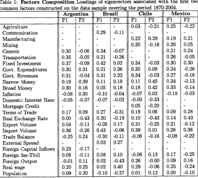
Table 1 shows the estimated factor loadings for the first two factors extracted using

the Stock and Watson procedure and the HP-detrending since·the results using other

methods yield very similar estimates, as shown below. We report only the first two

factors since the addition of further factors only contributes marginally to the total variance of the panel with the exception of one country (Brazil) for which the third factor is important (more on this below). The first factor (labeled FI) can be interpreted as a broad measure of cyclical activity since it loads positively on indicators that are well-known to be procylical such as sectorial output, fixed capital formation, import

quantum and real money, aIl measured in deviations from their respective long-term

trends. The interpretation of the second factor (F2) is less clear-cut. For Argentina, Brazil and Chile, this factor assigns large loadings to money, the domestic interest rate and the real exchange rate (also entered in deviations from trend). Thus, it can

be broadly interpreted as an index of monetary conditions. In the case of Mexico,

the largest loadings are observed on the variables capturing externallinkages such as the term of trade, the real exchange rate or import volume. This is suggestive of an important difference between the economies, possibly indicating that Mexico's linkage

to the US economy is of special relevance - a hypothesis that is corroborated by further

evidence presented below.

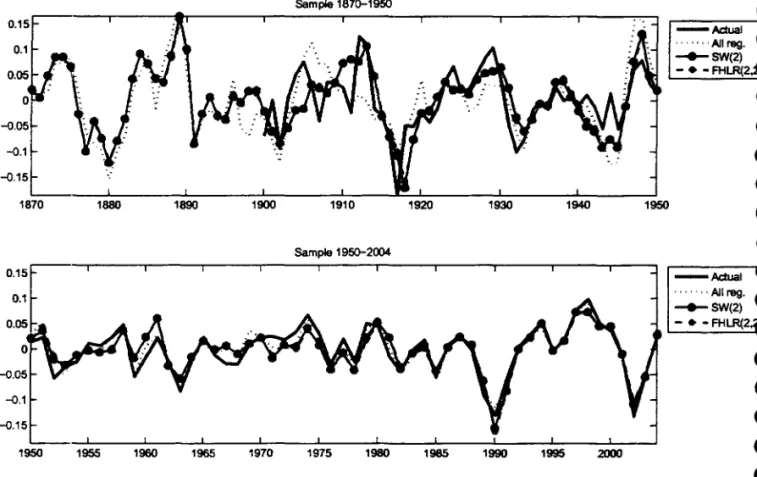
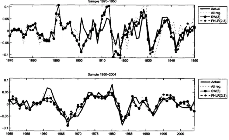
Figure 1 plots the two SW factors for each of the countries using the HP detrending

as reported in Table 1. For comparison, we also plot the same factors using band-pass

filter detrending. Since the two approaches yield very similar results, and given that the

HP-detrending does not entailloosing three annual observations on each extremes of the

sample and has been more extensively used in related studies (Backus and Kehoe, 1992;

Kydland and Zarazaga, 1997; Neumeyer and Perri, 2(05), we maintain this detrending

method through the remainder of the paper.

(15)

l

•

,

'.

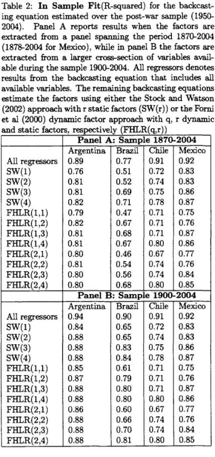
While the factors are of interest in their own right, ultimately our interest lies in reconstructing a measure of cyclical activity in the Latin American economies. To this end, Table 2 reports the R-value of regressions of de-trended actual GDP on the factors across a range of factor model specifications. The results cover the period ＱＹｾ＠ 2002, when full national account estimates are available for all four countries. As with the bulk of the series entering the alternative factor specifications, actual GDP is also expressed in deviations from an HP trend - a widely used measure of the output gap. Correlations in Table 2 thus gauge the extent to which the various factor models span

the real GDP cycle. To indicate the sensitivity of the results to the adopted econometric methodologies, we present results both for the all regressor approach-which maximizes the

R

2 by projecting cyclical GDP on all variables-and a range of alternative factor approaches such as the Stock and Watson approach using between one and four common factors and the Forni et al (2000) approach estimated with up to two dynamic factors and up to four static factors. As we shall see later, the high in-sample fit of the all-regressor, 'kitchen sink' approach comes at the cost of overfitting the data and producing poor out-of-sample performance.

Over the period 1870-2004, the linear projections of GDP growth on the various factors yield a tight fit for Argentina, with

.R

2_-values_varying_{from 0.89 for the}

all-regressor approach to around 0.80 for the two factor approaches Correlations are also generally high for Chile and Mexi.co, with ＷｾＸＵ＠ percent of the variance of the real GDP cycle explained by the first two factors. The fit for Brazil is relatively WOISe, as indicated

by

.R

2_{-values in the}_{ＰＮｾＰＮＷＰ＠} _{range. Only by including the series on agricultural and}

manufacturing output (both of which are onlyavailable from 1900 onwards), can one raise the fit of the regressions for Brazil to above 70 percent using the SW and the FHLR approaches, c.f. panel B of Table 2.

F\rrther evidence that the various approaches tell a simjlar story can be gleaned from Figures 2-5, which show the backcast estimates of cyclical GDP in the four economies.

In each case the upper panel plots the estimates and (where available) actual values of cyclical GDP over the period 1870-1949, while the bottom panel shows the correspond-ing values for the remaincorrespond-ing part of the sample. The close proximity between the fitted and actual values for the post-war period is clear from these plots-visual dilferences onlyemerge during rare and extremely large spikes such as in Brazil in 1961-62 and

14

• _•

•

• _•

•

• _•

•

• _•

•

• _•

•

• _•

•

• _•

•

• _•

•

• _•

•

(16)

•

• _•

• _s

•

• _s

.,

•

• _•

•

• _•

•

• _•

•

• _•

s

1980.7 Overall, however, it is pIain that: (i) the estimated values dosely track actual

cyclical GDP whenever this is available; (ü) the various factor approaches generate quite

similar estimates of the cyde and

(ili)

factor estimates often differ substantially from

estimates based on the all-regressor least squares approach whicb. in turn is furthest

away from the actual value. This strongly cautions against the use of "kitchen sink"

approach by previous researchers in the reconstruction of earlier GDP data.!l

3.2 Robustness Analysis: Parameter Instability

and

Fador

Specmcation

It is important to investigate whether our estimates are robust to potential instability of the factor loadings and to changes in the factor specification. The common factor projections were built under the assumption that factor loadings remain constant over

time. In the same way that out-of-sample forecasts rely on an implicit assumption

that certain relationships between predictor variables and the target variable remain constant over the forecasting period, backcasting economic activity measures without this assumption is infeasible.

An advantage of our approach is that the use of common factoIS can be expected

to be reasonably robust against the structural instability that plagues low-dimensional forecasting regressions. Stock and Watson (2002) provide both theoretical arguments and empirical evidence tbat principal component factor estimates are consistent even in

the presence of temporal instability in the individual tim&series used to construct the

factoIS provided that this instability averages out in the construction of the common

factoIS. This occurs if the instability is sufficiently idiosyn.cratic to the various series.

To evaluate the robustness of our results for the backcasted GDP values, Figure 6

plots the rojnjroum and maxim.um value across different specifications of the backcasting

7The gaps between the "actual" values and our backcast estimates for Brazil before 1930 should not been seen as misses since what is denoted as actual is the Haddad (1978) estimate which, as noted above, is constructed with incomplete sectoral data and relies extensively on interpolation and use of regression analysis to fill gaps in the actual output series. Given the reasonably tight fit between our index and the oflicial GDP data after 1950, we suspect that such apparent misses reflect the inaccuracies of the Haddad index rather than of our index, which relies on information across a wider spectrum of variables.

8 As mentioned above, this approach has been used by della Paolera (1988) to backcast Argentine

GDP during 1884-1899. It has also been used by Braun et a!. (2000, p.20) to backcast Chilean GDP for much of the 19th century.

(17)

equation. In particular we consider:

• Two different estimation samples for the backcasting equation, 1915-2004 and

1950-2004 (GDP data for Chile and Mexico are available only after 1940 so for

these countries the backcasting equation is estimated only over the sample 1950-2004.)

• Sixdifferentfactorspecifications: SW(2), SW(3), FHLR(2,1), FHLR(3,1), FHLR(2,2), FHLR(2,3).

• Different samples for factor estimation, where a new sample occurs if new time

se-ries become available (Argentina: 2004, 1875-2004, 1900-2004;Brazil: 1870-2004, 1900-2004; Chile 1870-2004; Mexico: 1878-2004).

• Two different panels of data, one including the external variables while the other excludes these.

The sensitivity analysis produces 72 specifications for Argentina, 36 for Brazil and 12 for Chile and Mexico. With the exceptions of Brazil in 1890-91, 1986 and 1989, and Chile in 1929-32 and Mexico in 1916, the range is very narrow; and even at those outlier

observations, all estimates point in the same direction. .Ai:. it turns out, all indications

are that little has ebanged over time. This congruence would be unlikely to hold if the

factor loadings were subject to structural breaks or considerable instability.

Overall, the results above make a simple but important point. Even when the

common factors are extracted from a dataset containing limited information on output

growth, they track the real GDP cycle well. This may not be overly surprising since we

selected variables that economic theory suggests should be closely related to cyclical activity. Yet, tbis evidence underscores the robustness of backcasting inferences on the aggregate output cycle using simple combinations of a cross-section of fiscal, financiaI, sectorial and external variables.

3.3 Gains from Using Extended Data Set

Although our results do not appear to be sensitive to the particular choice of factor

estimation metbodology, number of factors or sample period used to estimate the factor

loadings, one might ask what the 'value-added' is of using as wide a set of variables as

16

• _•

•

• _•

•

• _•

•

• _•

•

• _•

•

• _•

•

• _•

•

(18)

•

• _•

•

5 S

•

• _•

•

• _•

•

that adopted here when constructing the common factors. To answer this, we compare

in Figure 7 plots of the first common factor constructed using our extensive data set

vs. that using only sectoral output variables. This comparison shows the value from

including information on financia!, fiscal and trade variables. The differences are not negligible. Common factors based exclusively on sectoral output data are far smoother than those based on the wider set of variables. This shows up in a failure of the more narrowly constructed common factors in fully accounting for the depth of the crises in Argentina in 1918 and 1990, in Brazil and Mexico following World War I and in Chile

following the Great Depression. In addition many of the smaller peaks and troughts

-such as the cycle around 1900 in Argentina - are entirely missed by the common factor

based on sectoral output information.

Notice also that this limitation of the smaller set is not exclusive to Argentina

for which we have only two sectoral variables going back to 1870. Adding industrial output for Argentina (a series that becomes available from 1875) does not overtum this

conclusion. Significant ｧ｡ｾ＠ also arise for Brazil, Chile, and even Mexi.co which has

a wider sectoral output data converage all the way back to the 1870s. F\rrther, the

discrepancies between the two series are not exclusive to the pr&-war period, and hence do not seem entirely attributable the poorer quality of earlier data; large gaps emerge, for instance, for post-l960 Brazil.

These plots vividly demonstrate the importance to the construction of broad

mea-sures of economic activity of using a wide and varied set of economic variables

repre-senting not just a few sectoral output series. As one might expect, fiscal, financiai and externaI trade variables have a non-negligible role in filling the gap.

4 Thacking

History

We next ask how well the backcasted series square with qualitative historical evidence on

events deemed to be major economic tuming points in these countries. Figure 8 relates

the two. Starting with pre-war Argentina, the index picks up all economic downturns

associated with well-known world events - notably the stock market crashes in Europe

and the US in 1873 and the ensuing global economic depression, the 1890 Barings crisis,

the 1907 financiai panic, the two world war8, and the Great Depression of the 19308.

Likewise, major pa:;t-WWII shocks are also conspicuously pick.ed up as turning points

(19)

!

• ,

t

I

,

r

!

.

_ｾ＠

in our index, notably the boom and bust in world commodity prices 8SSOCiated with

the Korean War in the early 1950s, the oi! price shocks of the 1970s, the early 1982-83

debt crisis, as well as the emerging market crises of the 1990s (the 1994-95 "Tequila"

crisis and the Asia and Russia crises of 1997-98). A glance at Figure 8 also indicates that such a juxtaposition of cyclical turning points in country indices with major world

economic events is broaclly corroborated for Brazil, Chile, and Mexico.9

In addition, the portrait of history provided by our index: is consistent with narrative

evidence about the macroeconomic repercussions of key country-specific events. In the

case of Brazil, the index: picks up the mini downturn associated with the 1888 political unrest (end of Slavery and the republican transition) as well as the subsequent boom (the "Encilhamento") stemming from a liberal monetary reform that brought about an unprecedented boom in domestic credit and asset valuations in 1889-90 (see llinner,

2(00). The Brazil index: tracks equally well what is deemed to have been one of Brazil's

most protracted recessions which Cl1]minated in the country's first sovereign default and the debt rescheduling arrangements under the auspices of the Rothchilds in 1898 (see

Fritsch, 1988).10 As for Chile, our index highlights the upturn of 1879-82 associated

with the "War of the Pacific" (against Peru), the downturn around the country's exit

from the gold standard in 1898 (Llona Rodriguez, 20(0), as well as the severity of the

1929-32 depression in Chile due to plummeting terms of trade (Diaz.-Alejandro, 1984). Both in Argentina and Chile as well as (to a lesser ex:tent) Brazil, the index: identifies clear turning points around the military coups of the 1960s and 19708.

Finally, the Mexico index: yields a picture of economic fluctuations that is

remark-ably consistent with that depicted by Mexican historiography starting with the 1879-82

upturn that is typically associated with the onset of the new regime headed by General

Porfirio Diaz (Cardenas, 1997). Likewise, the subsequent recession is clearly depictedj

with the 1885 trough coinciding precisely with the well-documented austerity plan

im-9In contrast with Argentina, Brazil and Chile were little affected by the 1994-95 Mexican crisis partly due to offsetting domEStic developments. In the case of Brazil, a singularly successful stabilization plan in 1994 and renewed political stability set off a domestic demand boom in the following year. In the case of Chile, stronger trade linkages with Asia, low public debt, and a significant improvement in externaI terms of trade limited the disruptive effects of Tequila crisis on the domestic economy (see Singh et aI., 2005).

lOUnlike severa! Latin American countries which defaulted on their externai debts (and some also on their domestic debts) more than once throughout the 19th century, Brazil copiously serviced its sovereign debt obligations until then (Summerhill, 2004).

18

• _•

•

• _•

•

• _•

•

• _•

•

(20)

•

• _•

••

•

• _•

•

• _•

•

• _•

•

• _•

•

• "

<..

posed by Diaz's finance minister Manuel Dublan that involved a temporary suspension

of payments on domestic public debt; this was followed by an upswing that coincided

with Mexico's renewed access to international capital markets in the wake of the ＱＸＸｾ＠

87 externaI debt settlement and the resumption of strong capital inflows in the late

1880s (c.f. Marichal, 2002). This strong upswing was brought to a ha1.t by a sharp

worldwide fall in silver prices (Mexico's main export item) coupled with a sudden stop

in capital fiows to emerging markets in the early 18908 (c.f. Catão and Solomou, 2(05)

Finally, our business cycle index also provides a new measure of the severity of the

economic downturn associated with the Mexican Revolution of 1911-20 identifying a trough around 1915-16-these were the years when the revolutionary confiict peaked and chaotic monetary conditions triggered a hyperinfiation (Cardenas and Manns, 1988).

4.1 Business

Cycle Dating

Armed with the business cycle indicators for the four countries, we turn to the task

of formally dating the respective turning points. A classic device to this end, which

is also consistent with our definition of the business cycle as output deviations from

a stochastic or deterministic trend, is the Bry and Boscham (1971) algorithmY It

consists of a sequence of procedures starting with the search for extreme values in order to e1iroinate (near-)permanent jumps in the series associated say with outliers, followed by the use of centered moving averages of the series and the search for local maxima

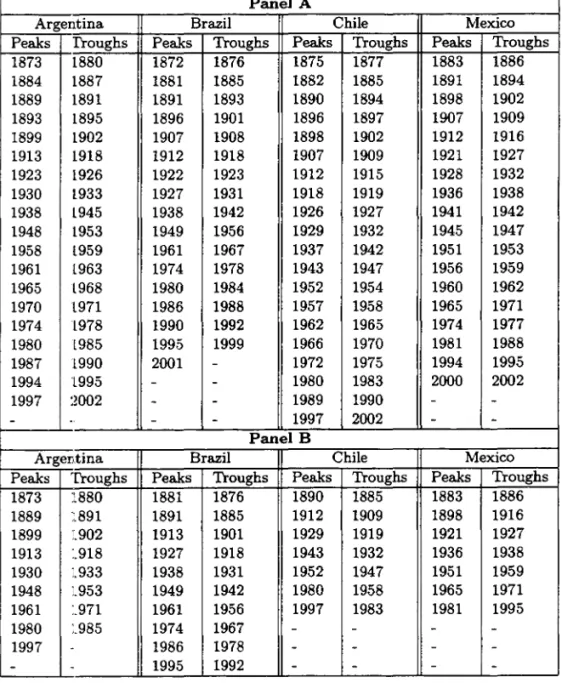
or roiniroa within a chosen window length.12 _Panels_A_and_B_{of Table}₃_{report results}

based on two-year and three-year windows, respectively. As expected., the algorithm

identifies peaks and troughs that are broadly consistent with a visual inspection of

Figures 2-8. When the narrower window is used, the average duration of the cycle is

11 A recent alternative dating procedure which al50 builds on the Bryand Boschan approach has been

advanced by Harding and Pagan (2004). Their procedure has been designed for use with quartely data and growth cydes rather than with measures of the output gap. As discussed in Marcellino (2005), measuring the cyde as deviations from trend as we do is a more suitable procedure in contexts where absolute declines in output are not 50 rare, as in our group of countries over the past century. Conversely, the concept of a growth cycle is more analytically relevant when absolute declines in output are very rare and growth rates are reasonably persistent, as in Western Europe in the early post-war decades. Most of the recent empirical literature on business cycle identification and measurement has focused on the classical cycle defined in terms of deviations from trend (stochastic or deterministic).

12See King and Plosser (1984) and Watson (1994) for further details and application to US data, for

which the algorithm closely replicates the dating by the NBER's panel of experts.

(21)

shorter overall, and the more so when one focuses on the post-war era. This finding is consistent with evidence of the shortening business cycle length among advanced

countries

(see,

e.g., Gordon, 1986) Using a longer window, Pane! B indicates that

the pre-cycle is dominated by the Kuznets or long swings, with similar tuming points

as those identified in the literature on Anglo-saxon economies (Solomou, 1987). This

evidence is further reinforced by spectral density function estimates of the individual

country indices, which point to a domjnant cyclicallength around 14 to 16 years during

the 1870-1930 period (a typical Kuznets-swing length), followed by a 10-12 year cycle

in pa;t-war data (Table 4).

In sum, both the Bry and Bosham algorithm and the spectral density function

estimates point to a reasonably long average cyclical duration in all four countries. The domjnant cyclical pattern was generally longer in the pre-1930 era, but even in the

pa;t-World War II period, cycles in Latin America were substantially more protracted

than in the United States and other advanced countries.13

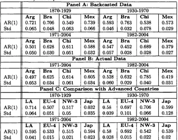
Against this background, Tables 5 and 6 report a set of descriptive statistics that

he!p characterize other stylized facts about Latin America's business cycles. First, standard deviations corroborate the perception that Latin America has been a more cyclically volatile region than both countries deemed advanced by today's definition as

well as countries such as Australia, Canada and Japan that were considered "emerging

economies" in the pre-war world. This volatility gap between the two groups has

changed over time, however. The four Latin countries were clearly far more volatile in

the early globalization period before the 19308 - characterized as it was by free capital

mobility and very limited quantitative restrictions on trade. Conversely, there is prima

facie evidence tha.t the inward growth policies did succeed in fending these countries oif global instability in the 1930-70 sub-period, when global volatility generally rose, partly due to the recovery from the 1929-32 depression and war shocks, which appear re.flected in the higher standard deviation of the output gap among advanced countries during the period. But as output gap volatility came down in advanced countries in the

pa;t-1960s period (notwithstanding two oil shocks and dramatic changes in economic

policies), cyclical volatility in Latin America remained relatively high; only in the

pa;t-I3To the extent tha.t the combination of large shocks and high cyclical persistence make the task of stabilization policies more difficult, this finding has interesting implications for the interpretation of the history of stabilization policies in Latin America.