A NEW CLASSIFICATION OF ROMANIAN COUNTIES BASED ON A COMPOSITE INDEX OF ECONOMIC DEVELOPMENT
Zaman Gheorghe 1, Goschin Zizi 1,2
1Institute of National Economy, Romanian Academy, Bucharest, Romania
2Departmentof Statistics and econometrics, Bucharest University of Economic Studies, Romania
[email protected] [email protected]
Abstract: This paper is dealing with the problems concerning the improvement of regional classifications by using a composite index of economic development which encompasses four individual indicators: GDP/capita, labour productivity, FDIs and life expectancy. Our aim is to offer a better methodology and a multi-sided image on the regional development,
from the perspective of two major factors of influence: Romania’s accession to EU and
the recent economic crisis. A special attention should be paid to the hierarchical position of each influence factor. Depending on the specific factor mix, we try to draw conclusions regarding the relationship between economic resilience and vulnerability of each regional
economy. The new approach based on the composite index’s computation has the
advantage of providing a unique answer on problems such as unclear hierarchies or even contradictory results emerging from different classifications that use separate indicators. The study is covering the 2001-2012 period, divided into two sub-periods: 2001-2006 (pre-accession) and 2007-2012 (post-(pre-accession).
Keywords: economic development, composite index, classification, regions, Romania
JEL classification: O18, R11
1. Typological categories of regional growth and decline
Regional science has imposed widespread use of rigorous methods for analyzing phenomena and processes where space plays a significant role. Analysis of territorial growth profiles for a medium-developed country like Romania raises different issues compared to developed countries (Barca et al., 2005; Dincă, 2005; Banciu, 2006; Constantin and Constantinescu, 2010; Ailenei et al., 2012; Antonescu, 2012). It is about the different stages of the process of sustainable economic growth, which in the case of Romania rather reflect the increase of relative and absolute gaps. It is important that these rising disparities take place in the context of economic performance increases, both regionally and locally. From the perspective of regional statistics, Romania is currently an assembly of eight development regions NUTS 2, of which seven are below 75% of the EU-28 level of GDP per capita. This requires a thorough multicriterial analysis of regions’ specificities and inter-regional disparities, although territorial disparities are lower in Romania than in many other European Union countries (Goschin et al., 2008; Nahtigal, 2013).
The theoretical and practical interest of the method applied in this paper consists in the possibility of combining the static and dynamic analysis for performing a comparative analysis of regional levels of one result variable against the average at national level at a certain moment (static aspect), as well as for comparing the evolution in time (growth rate) of regional levels against the national average (dynamic aspect).
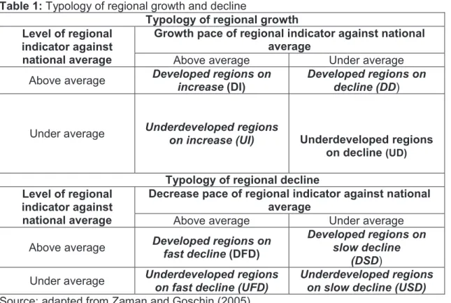
This typology of regional growth might be employed for any result indicator recorded at regional level by using the absolute level of the indicator at a certain moment, as well as the growth rate of the same indicator for a given period. Correlating this information, each region is included into a certain type of economic evolution (Table 1) depending on the position it holds in relation to the average level and dynamics of the national economy.
Table 1: Typology of regional growth and decline
Typology of regional growth Level of regional
indicator against national average
Growth pace of regional indicator against national average
Above average Under average
Above average Developed regions on increase (DI)
Developed regions on decline (DD)
Under average Underdeveloped regions
on increase (UI) Underdeveloped regions on decline (UD)
Typology of regional decline Level of regional
indicator against national average
Decrease pace of regional indicator against national average
Above average Under average
Above average Developed regions on fast decline (DFD)
Developed regions on slow decline
(DSD)
Under average Underdeveloped regions on fast decline (UFD)
Underdeveloped regions on slow decline (USD) Source: adapted from Zaman and Goschin (2005)
In order to characterise the economic development at regional and national levels a widely used indicator is the Gross Domestic Product, which represents a barometer for the favourable/unfavourable evolution of the economy. When the result indicator (GDP) is associated to population, at regional and national levels (for instance under the form of GDP per capita) we obtain a sui-generis image of the economic-social development level. When GDP is associated to an effort indicator (for instance employment, investments, fixed assets, research-development expenditures, etc.), we obtain an assessment of the regional and national efficiency and development level, useful for understanding the synthetic economic effects achieved as a result of resources consumption lato sensu. Applied to concrete data for various regional disaggregation levels, this method confers to decision makers information for designing the economic policy mix based on the ranking of each region into a certain type of economic evolution.
When the regional typology is defined as depending on the GDP per capita indicator, the level of the indicator on each region (GDPR/cap) is compared to the national average (GDP/cap), and the percentage growth of GDP per capita at regional level (RGDPR/cap) to
As result of corroborating the regional level and dynamics of GDP/capita against the national ones, we obtained four regional categories for which the main characteristics shall be presented in the following.
a) Developed regions on increase are placed above the national average as regards both the absolute level of the indicator (GDPR/cap >GDP/cap) and its dynamics (RGDPR/cap
> RGDP/cap.). These regions practically rise to economic decision making process the issue
of continuing to maintain the swift dynamic on different time horizons, so as to avoid the overheating phenomenon, as well as the risk of slow-down and decline. In this context it is necessary to take into account the possible impact of the business cycle, the determinants of which might be of economic-social nature, but of technological or environmental nature as well. As a rule, these regions have a strong driving effect and are regarded as growth “engines” for the overall economy.
b) Developed regions on decline have a GDP per capita level higher than the national average (GDPR/cap > GDP/cap), but their growth rate is below average (RGDPR/cap <
RGDP/cap). This slowness is caused by various factors whose action could no longer be
offset and lay in front of the decision makers the need to restructure the existing activities and to create some new competitive activities with positive effects.
c) Underdeveloped regions on increase are those aiming to recover the gaps against the mean level of GDP per capita by having a growth rate above the average one (GDPR/cap < GDP/cap and RGDPR/cap > RGDP/cap). Their future development strategy needs
to maintain a dynamic that allows to partially or entirely recover the gap and even to exceed the average level, which could allow them to enter the category of developed regions on increase.
d) Underdeveloped regions on decline have a GDP per capita level below average, but cannot diminish or recover this gap because their growth rate is lower than the national mean (GDPR/cap < GDP/cap and RGDPR/cap < RGDP/cap). As a consequence, the distance
separating them from the average is continuously growing, these regions representing the most unfavourable case, to which special attention should be paid, because the worsening of their economic-social situation might unfavourably influence the entire national economic complex. The problem of underdeveloped regions is chronic and requires state’s support at local and regional levels, as well as the creation of an attractive business climate for foreign investments, through economically developed areas, technological parks, free zones, etc.
These underdeveloped regions are a priority to the macroeconomic decision board from the viewpoint of stimulating private business, and avoiding possible critical crisis situations and social tensions. In addition, the issue of investments in education and social fields emerges, and it cannot be solved but by means of some efficient public-private partnership schemes, taking into account that the private sector usually is targeting only the profit.
An absolutely special interpretation, in the frame of the depicted regional typology, would require the cases in which the growth level and/or rhythm from a region is equal to the national one, resulting some particular situations: average level regions on increase (GDPR/cap =GDP/cap and RGDPR/cap > RGDP/cap) or on decline (GDPR/cap =GDP/cap and
RGDPR/cap < RGDP/cap) that reached an average level of GDP per capita either by climbing
up the regional hierarchy from the position of underdeveloped region, or downgrading from the category of developed region; stagnant developed regions (GDPR/cap > GDP/cap and RGDP/cap= RGDP/cap) that maintain their relative advantage comparatively to
the average without recording either progress or decline in the regional hierarchy; underdeveloped stagnant regions (GDPR/cap < GDP/cap and RGDPR/cap = RGDP/cap)
In the above mentioned cases, a particular practical importance has the quality of economic growth. If the national average growth is high enough, then we might qualify as satisfactory the evolution of regions placed around this average. To the contrary, if this average is low, the regions coming close to it cannot be regarded as finding themselves in a favourable economic-social situation. A case with obvious negative connotations for regions close to the average is when the growth rhythm at national level is negative. A particular situation within this methodology emerges when the economy is on decline at regional and national levels, and we need to reinterpret the typology under new circumstances. From the perspective of economic recovery strategy and in view of solving economic crises’ problems, the identification and monitoring of various cases of economic decline are also important (Table 1).
Since a single indicator is not enough for characterising and classifying complex entities such as the regional economies, we are further going to put together four regional variables in order to build a composite index of economic development. In view of compatibility between the selected variables, a normalization procedure should be applied first. Original data on each indicator is transformed as follows:
)
min(
)
max(
)
min(
jt jt jt ijt ijtx
x
x
x
y
-=
, (1)
where:
yijt - the normalized value of indicator j for region i in year t;
xijt - initial value of indicator j, region i and year t.
Converted values range from 0 (worst case) to 1 (best case) for each region/county and for all four indicators.
The composite index of economic regional development (CED) is computed using the weights pj for normalised values on each variable j.
.
100
3 1å
=×
=
j j ijt itp
y
CED
(2)The weights of the four standardized variables included in the composite index are as follows: GDP per capita-30%, labour productivity – 20%, FDI -15%, life expectancy -35%. These weights are not exclusive, they might be changed according to different priority settings or preferences.
2. Typological categories of Romanian counties
of variation can range between 0 and
n
-
1
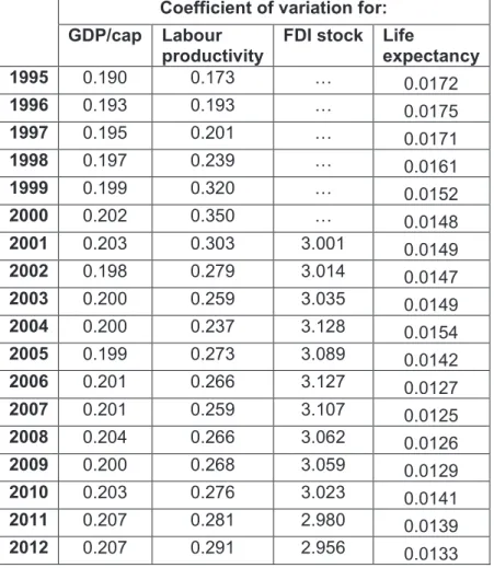
, n being the number of terms in statistical series (number of territorial units in our case). The higher is CV, the more dispersed is the variable. Above unit values, less frequent in the case of economic variables, are indicating a high level of dispersion. Percentage expression of the coefficients of variation can be misleading because the value of CV may exceed unity, resulting percentages higher than one hundred. Therefore we prefer the adimensional form of CV.Table 1: Annual coefficients of variation for GDP/cap, labour productivity, FDI stock and life expectancy, 1995-2012
Coefficient of variation for:
GDP/cap Labour productivity
FDI stock Life
expectancy
1995 0.190 0.173 … 0.0172
1996 0.193 0.193 … 0.0175
1997 0.195 0.201 … 0.0171
1998 0.197 0.239 … 0.0161
1999 0.199 0.320 … 0.0152
2000 0.202 0.350 … 0.0148
2001 0.203 0.303 3.001 0.0149
2002 0.198 0.279 3.014 0.0147
2003 0.200 0.259 3.035 0.0149
2004 0.200 0.237 3.128 0.0154
2005 0.199 0.273 3.089 0.0142
2006 0.201 0.266 3.127 0.0127
2007 0.201 0.259 3.107 0.0125
2008 0.204 0.266 3.062 0.0126
2009 0.200 0.268 3.059 0.0129
2010 0.203 0.276 3.023 0.0141
2011 0.207 0.281 2.980 0.0139
2012 0.207 0.291 2.956 0.0133
Source: authors’ computations.
Calculations of coefficients of variation for GDP/capita, productivity, life expectancy and the stock of FDI, on an annual basis, in the period 1995-2012 (Table 1) reveal the following:
· changes in territorial per capita GDP are less marked than the variation in productivity and have higher stability, which can be explained by higher territorial variability of employment against total population, mainly as a result of external migration; the dispersion of GDP/capita follows a slightly upward trend, indicating steady increase in disparities at the county level during 1995-2012;
reversed in the next period, amid strong economic growth in 2001-2007, but resumed since 2008;
· the large values of the annual coefficients of variation calculated for the foreign direct investments stock over 2001-2012 show an extremely high level of territorial inequalities; CV enrolled on a slightly downward trend since 2006, the decrease being more pronounced in recent years in the context of severe decline in FDI inflows as a result of the economic crisis; it is worth mentioning that the variations in FDI inflows depend not only on domestic fluctuations, but also, to a larger extent, on numerous external factors of influence.
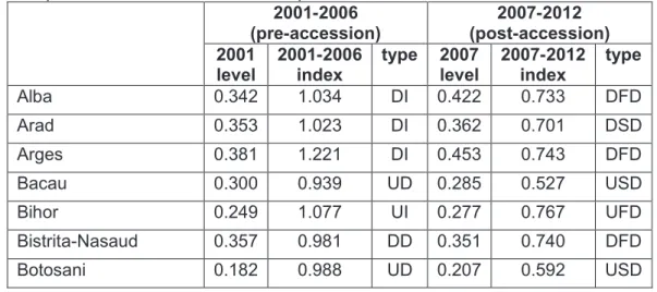
The level and dynamic of the composite index of economic development calculated for the Romanian counties over 2001-2012 showed that Bucharest Municipality was constantly placed on the first position. The typological categories of the Romanian counties for the period 2001-2006 (pre-accession) are as follows (Table 2):
· Developed counties on increase (DI): Alba, Arad, Arges, Cluj, Constanta, Ilfov, Prahova, Sibiu, Timis;
· Developed counties on decline (DD): Bistrita- Nasaud, Brasov, Buzau, Covasna, Galati, Gorj, Harghita, Bucharest Municipality, Mures, Suceava and Valcea;
· Underdeveloped counties on increase (UI): Bihor, Braila, Dambovita, Ialomita, Iasi, Maramures, Neamt, Tulcea, Vrancea;
· Underdeveloped counties on decline (UD): Bacau, Botosani, Calarasi, Caras-Severin, Dolj, Giurgiu, Hunedoara, Mehedinti, Olt, Salaj, Satu Mare, Teleorman, Vaslui represent the largest group.
The typological categories of the Romanian counties for the period 2007-2012 (post-accession) are:
· Developed counties on slow decline (DSD): Prahova, Iasi, Gorj, Arad, Covasna, Constanta;
· Developed counties on fast decline (DFD): Alba, Suceava, Bistrita-Nasaud, Arges, Sibiu, Vrancea, Cluj, Ilfov, Dambovita, Timis, Brasov, Valcea, Bucharest Municipality;
· Underdeveloped counties on slow decline (USD): Tulcea, Braila, Bacau, Ialomita, Mehedinti, Satu Mare, Botosani, Vaslui, Teleorman, Neamt, Galati, Buzau, Salaj, Calarasi, Mures;
· Underdeveloped counties on fast decline (UFD): Harghita, Dolj, Hunedoara, Caras-Severin, Bihor, Maramures, Olt, Giurgiu.
Table 2: Typological categories of the Romanian counties over 2001-2012 according to the composite index of economic development
2001-2006 (pre-accession) 2007-2012 (post-accession) 2001 level 2001-2006 index
type 2007 level
2007-2012 index
type
Alba 0.342 1.034 DI 0.422 0.733 DFD
Arad 0.353 1.023 DI 0.362 0.701 DSD
Arges 0.381 1.221 DI 0.453 0.743 DFD
Bacau 0.300 0.939 UD 0.285 0.527 USD
Bihor 0.249 1.077 UI 0.277 0.767 UFD
Bistrita-Nasaud 0.357 0.981 DD 0.351 0.740 DFD
Braila 0.321 1.025 UI 0.345 0.520 USD
Brasov 0.505 1.006 DD 0.534 0.825 DFD
Buzau 0.350 0.897 DD 0.333 0.692 USD
Calarasi 0.201 0.826 UD 0.183 0.701 USD
Caras-Severin 0.254 0.929 UD 0.248 0.748 UFD
Cluj 0.466 1.025 DI 0.529 0.767 DFD
Constanta 0.343 1.258 DI 0.394 0.725 DSD
Covasna 0.432 0.765 DD 0.350 0.704 DSD
Dambovita 0.315 1.022 UI 0.354 0.777 DFD
Dolj 0.289 0.947 UD 0.295 0.741 UFD
Galati 0.375 0.862 DD 0.334 0.660 USD
Giurgiu 0.244 0.686 UD 0.150 0.999 UFD
Gorj 0.416 0.985 DD 0.448 0.674 DSD
Harghita 0.375 0.890 DD 0.334 0.739 UFD
Hunedoara 0.282 0.947 UD 0.288 0.746 UFD
Ialomita 0.268 1.022 UI 0.254 0.533 USD
Iasi 0.327 1.043 UI 0.366 0.658 DSD
Ilfov 0.499 1.304 DI 0.595 0.771 DFD
Maramures 0.180 1.200 UI 0.225 0.783 UFD
Mehedinti 0.289 0.809 UD 0.242 0.567 USD
Bucharest Municipality 1.000 1.000 DD 1.000 0.957 DFD
Mures 0.348 0.936 DD 0.332 0.712 USD
Neamt 0.274 1.116 UI 0.323 0.631 USD
Olt 0.280 0.665 UD 0.216 0.905 UFD
Prahova 0.384 1.161 DI 0.460 0.654 DSD
Salaj 0.222 0.990 UD 0.253 0.694 USD
Satu Mare 0.099 0.943 UD 0.087 0.576 USD
Sibiu 0.415 1.054 DI 0.455 0.760 DFD
Suceava 0.342 1.005 DD 0.359 0.734 DFD
Teleorman 0.294 0.671 UD 0.227 0.599 USD
Timis 0.441 1.160 DI 0.515 0.796 DFD
Tulcea 0.128 2.103 UI 0.248 0.285 USD
Valcea 0.433 0.950 DD 0.428 0.954 DFD
Vaslui 0.222 1.000 UD 0.241 0.592 USD
Vrancea 0.296 1.189 UI 0.352 0.763 DFD
Average 0.335 1.008 0.349 0.729
As it results from the comparative approach of the two sub-periods, the main conclusion which could be drawn is that the global impact of the economic crisis that hit the Romanian economy could not be countered by the expected benefits of integration and advantages of the enlarged EU market. Even worse, some state that the impact of crisis and integration is overlapping in the same negative direction because, as it is revealed by the experience of new-comers to EU, there is an period of accommodation and difficult interface between the new members and EU market rigours, resulting in initial economic decline as the price paid for integration.
It is not less important to acknowledge the territorial variation in the severity and duration of economic decline under the circumstances of a different set of vulnerabilities and resilience. The best example of resilience is the Bucharest Municipality, owing to its relatively high level of economic and social development. On the opposite, weaker resilience and higher vulnerabilities are specific for most counties in North-East and South-East of Romania because of their lower level of development. A factor having important impact on lower robustness for the developing areas of Romania is the negative influence of labour force emigration, especially from less developed zones, having scarce business and employment opportunities and low-paid jobs.
The main advantage of using a typology based on this composite index of development, instead of individual indicators, consists in a more complex, multi-sided approach of regional classification of economic and social development, but it is also noteworthy the potential loss of information, as bringing together several indicators may partially level the differences between counties.
4. Conclusion
The paper offered a new approach of regional classifications, based on a composite index of economic development which encompasses four individual indicators: GDP/capita, labour productivity, FDIs and life expectancy. The method has the advantage of providing a unique answer on problems such as unclear hierarchies or even contradictory results emerging from different classifications that use separate indicators. The study covered the 2001-2012 period, divided into two sub-periods: 2001-2006 (pre-accession) and 2007-2012 (post-accession). The results revealed that the two sub-periods display distinct trends, as the pre-accession period recorded a clear trend of overall economic growth, although the underdeveloped counties on decline represented the main group, while the second period was impacted by the effects of the global economic and financial crisis. The main conclusion which could be drawn is that the global impact of the economic crisis that hit the Romanian economy could not be countered by the expected benefits of integration in the EU market.
Bibliography
Ailenei, D., Cristescu, A., Vişan, C. (2012). ”Regional patterns of global economic crisis shocks propagation into Romanian economy”, Romanian Journal of Regional Science, 6(1), pp. 41-52.
Antonescu, D., (2012) "Identifying Regional Economic Disparities and Convergence in Romania," Journal of Knowledge Management, Economics and Information Technology, ScientificPapers.org, vol. 2(2).
Barca, F., Brezzi, M., Terrible, F., Utili, F., (2005) ”Measuring for Decision Making: Soft and Hard Use of Indicators in regional Development Policies”, OECD, http:/www.oecd.org/ oecdworldforum.
Constantin, D.L., Goschin, Z., G. Drăgan, (2010) “Implications of EU Structural Assistance to New Member States on Regional Disparities: The Question of Absorption Capacity”, capitol în R. Stimson, R.R. Stough, P. Nijkamp (editori), Endogenous Regional Growth, Edward Elgar Publishing Ltd., Cheltenham, UK, Northampon, MA, USA, pp. 182-203.
Constantinescu, M., D.L. Constantin, (2010), Dinamica dezechilibrelor regionale în
procesul de integrare europeană: modelare, strategii, politici, Editura A.S.E., Bucureşti
Dincă, C., (2005), Regionalizarea sau dilemele guvernării regionale, Editura Sitech, Craiova
Goschin, Z., D.L. Constantin, Monica Roman, Bogdan Ileanu, (2008), ”The Current State and Dynamics of Regional Disparities in Romania”, Romanian Journal of Regional Science, vol.2, no 2, pp. 80-105
INS, (2013), Baza de date online TEMPO, https://statistici.insse.ro/shop/
McCann, P. and Sheppard, S. (2003) ”The Rise, Fall and Rise again of Industrial Location Theory”, Regional Studies, 37 (6-7). pp. 649-663.
Myrdal, G., (1957), Economic Theory and Under – Development Regions, London, Duckworth.
Nahtigal M. (2013) ”European Regional Disparities: the Crucial Source of European Un -sustainability”, Evropska unija, no.4,
http://matjaznahtigal.com/wp-content/uploads/2013/04/SSRN_European-regional-disparities_March2013.pdf
Perroux, F., (1981) Pour une philosophie de nouveau development, PUF, Paris.
World Bank, (2009) World Development Report- Reshaping Economic Geography, New York
Zaman, Gh., Goschin, Z., Vasile, V. (2013) ”Evoluţia dezechilibrelor teritoriale din România în contextul crizei economice”, Romanian Journal of Economics, 2(46), pp. 20-39.
Zaman G., Georgescu G. (2009), ”The Impact of Global Crisis on Romania’s Economic Development”, Annales Universitatis Apulensis Series Oeconomica, 11(2).
Zaman, Gh., Goschin, Z. (2005) ”Tipologia şi structura creşterii economice regionale”,