Ensaios Econômicos
Escola de
Pós-Graduação
em Economia
da Fundação
Getulio Vargas
N◦ 769 ISSN 0104-8910
The Long-term Effects of Conditional Cash
Transfers on Child Labor and School
Enroll-ment
Marcel Peruffo, Pedro Cavalcanti Ferreira
Os artigos publicados são de inteira responsabilidade de seus autores. As
opiniões neles emitidas não exprimem, necessariamente, o ponto de vista da
Fundação Getulio Vargas.
ESCOLA DE PÓS-GRADUAÇÃO EM ECONOMIA Diretor Geral: Rubens Penha Cysne
Vice-Diretor: Aloisio Araujo
Diretor de Ensino: Carlos Eugênio da Costa Diretor de Pesquisa: Humberto Moreira
Vice-Diretores de Graduação: André Arruda Villela & Luis Henrique Bertolino Braido
Peruffo, Marcel
The Long-term Effects of Conditional Cash Transfers on Child Labor and School Enrollment/ Marcel Peruffo,
Pedro Cavalcanti Ferreira – Rio de Janeiro : FGV,EPGE, 2015 39p. - (Ensaios Econômicos; 769)
Inclui bibliografia.
The Long-term Effects of Conditional Cash Transfers on
Child Labor and School Enrollment
Marcel Peruffo
∗and Pedro Cavalcanti Ferreira
†August 11, 2015
Abstract
This paper investigates the long-term effects of conditional cash transfers on school attainment and child labor. To this end, we construct a dynamic heterogeneous agent model, calibrate it with Brazilian data, and introduce a policy similar to the Brazilian
Bolsa Fam´ılia. Our results suggest that this type of policy has a very strong impact on educational outcomes, sharply increasing primary school completion. The conditional transfer is also able to reduce the share of working children from 22% to 17%. We then compute the transition to the new steady state and show that the program actually increases child labor over the short run, because the transfer is not enough to completely cover the schooling costs, so children have to work to be able to comply with the program’s schooling eligibility requirement. We also evaluate the impacts on poverty, inequality, and welfare.
1
Introduction
This paper examines the long-term general equilibrium effects of conditional cash trans-fers (CCTs) on human capital accumulation and child labor. To this end, we construct a dynamic heterogeneous agent model that includes key determinants of child labor
∗Graduate School of Economics, Funda¸c˜ao Get´ulio Vargas
(e-mail: mcperuff[email protected]).
†Graduate School of Economics, Funda¸c˜ao Get´ulio Vargas, FGV Crescimento & Desenvolvimento (e-mail:
and school enrollment and then assess the effects of the Brazilian Bolsa Fam´ılia, an extensive conditional cash transfer program adopted in 2002. We calibrate the model using Brazilian data from various sources, including the Brazilian Household Survey
PNAD, and then compare two steady states: before and after the introduction ofBolsa
Fam´ılia. We also evaluate the transition across steady states and provide an alternative policy experiment.
Our model features a closed economy whose overlapping generations of dynasties care about consumption and child leisure. Idiosyncratic shocks to productivity induce families to save through a riskless asset, while borrowing constrains prevent them from investing optimally in human capital accumulation. As a result, a share of households is locked in a poverty trap, choosing to have their children work due to the very high marginal utility of consumption. In this environment, a conditional cash transfer policy can potentially alleviate poverty, induce school enrollment and discourage child labor. We model a conditional cash transfer program as a schedule of transfers and
school-ing requirements. Specifically, our transfer policy mimics the Bolsa Fam´ılia, whose
incentives depend on both income thresholds and on school enrollment. The schedule is set such that it matches the program’s coverage and budget (as a share of GDP) in 2012. Our model is calibrated to match main features of the Brazilian economy in 1997, before the widespread implementation of any conditional cash transfer program
in Brazil1.
Our results suggest that theBolsa Fam´ılia has a great impact on educational
out-comes: over the long-term, the program increases the share of children who complete at least primary school from 52% to approximately 90%. Additionally, the share of children who complete secondary school increases by 30% (from 33% to 41%), child la-bor hours are reduced by 20.4%, and the share of working children decreases by 22.5% (from 22% to 17%).
However, it is surprising to see that, during the transition to the new steady state,
the share of working children increases slightly over the short-term, reaching a peak
of 23% immediately after the intervention, compared to 22% before the introduction of Bolsa Fam´ılia. This happens because the transfer is not large enough to completely cover schooling costs, so children have to work more to be able to pay for their educa-tions and, thus, be eligible to receive the conditional transfer. As these children will become highly educated adults, their own children will not need to work. We observe that, after a time gap corresponding to one generation, the share of working children decreases to 17%, which is near the share working in the new steady state. This result
1
is not only consistent with the existing literature based on micro-evidence (Cardoso
and Souza (2004), Rocha and Soares (2009)2) but also suggests that the impacts of
Bolsa Fam´ılia on child labor reduction are forthcoming.
We also provide insights into the macroeconomic and distributional influences of such a transfer program. For instance, in spite of some sluggishness over the short run, the simulations predict that total output could increase by nearly 20% over the long-term. The initial sluggishness can be attributed to the “insurance effect” of a conditional cash transfer, but the benefits of an increasing workforce quality gradu-ally overcome the weaker precautionary motives. There is also a decrease in income inequality, as measured by the Gini coefficient of household income (5 points over the long-run).
Finally, we perform a welfare analysis. Our results suggest that only 33% of the population is better off immediately after the introduction of the new policy, with the welfare of the whole population decreasing by 2.26%. We then provide a counterfactual transfer policy using the same schedule except for a small amount of cash transferred to the very poorest families regardless of their decisions to send their children to school. In this case, the long-term benefits of the cash transfer program are slightly smaller in comparison with the benchmark policy, but the new policy is also able to reduce child labor over the short run and to increase welfare.
There is no lack of studies that examine the effects of conditional cash transfers programs on education, child labor, and poverty. With regard to the Brazilian case,
Barros et al. (2006) find that theBolsa Fam´ılia was responsible for 50% of the reduction
in inequality between 2001 and 2005. Additionally, Soares and S´atiro (2009) estimate
that this policy was responsible for a reduction of 8% in the poverty headcount ratio (1.7 percentage points), while Barros et al. (2010) claim that it was responsible for 15% of the observed reduction in extreme poverty between 2001 and 2008. In contrast,
Cardoso and Souza (2004) and Rocha and Soares (2009) find that theBolsa Escola had
no effect on child labor but increased the chances that a poor child attended school3.
In this work we focus on the impacts of the Brazilian CCT on child labor and ed-ucation. In our long-term analysis, comparisons with existing works should be made
carefully. For instance, many studies note that the Bolsa Fam´ılia slightly increased
educational attainment (Souza (2011)), but, to the best of our knowledge, there are
2
Duryea and Morrison (2004) also observe that a conditional cash transfer in Costa Rica had no impact on child labor.
3
no previous studies that investigate the future effects of the increase in human capital
accumulation on the Brazilian economy as a whole4. Our work fills this gap, as it looks
at differences in the economy across steady states equilibria.
Our work is related to the vast literature that measures the impacts of public poli-cies using simulations with heterogeneous agent models. Our model specifically builds on Restuccia and Urrutia (2004) and Krueger and Donohue (2004). We chose a general equilibrium framework to account for the price movements caused by a continuously
implemented new policy, which may play an important role in the programs effects5.
Our calibration makes use of data that precede the program’s existence. We then simulate a conditional cash transfer schedule that approximates the existing policy in terms of income threshold, schooling requirements, total coverage, and total budget.
In this spirit, Zilberman and Berriel (2012) inquire about the impacts ofBolsa Fam´ılia
on savings, inequality and adult labor supply. Our work differs from theirs because we focus on the effects on human capital accumulation and on child labor over the life cycle, features that are absent from their paper. Our work is closer to Cespedes (2010), who develops a life-cycle model that includes human capital accumulation, calibrating the model with data from Mexico and introducing a conditional cash transfer similar to the Mexican program, PROGRESA.
Another group of studies uses structural estimation to evaluate the effectiveness of public policies and to test them against counterfactual policies. In this context, the work by Todd and Wolpin (2002) stands out as particularly influential.
Bour-guignon et al. (2003) also perform a micro simulation of Bolsa Fam´ılia. An advantage
that these types of works share with ours is that they do not require experimental or quasi-experimental designs. However, our work differs from theirs not only due to the differences in the models used but also because their analysis abstracts from general equilibrium effects. Instead, in our work, price movements driven by aggregate human and physical capital have a considerable influence in the policy’s impacts over both the short and the long run.
The remainder of this paper is organized as follows: section 2 presents the model, section 3 describes our calibration strategy, section 4 features the results and provides a counterfactual experiment, and section 5 concludes.
4
With respect to this issue, Souza (2011) states that the existing studies find no effect on human capital accumulation. In fact, asBolsa Fam´ılia has only been recently implemented, the data generated until now is insufficient for a definitive analysis (Fiszbein et al. (2009)).
5
2
Model
2.1
Economic Environment
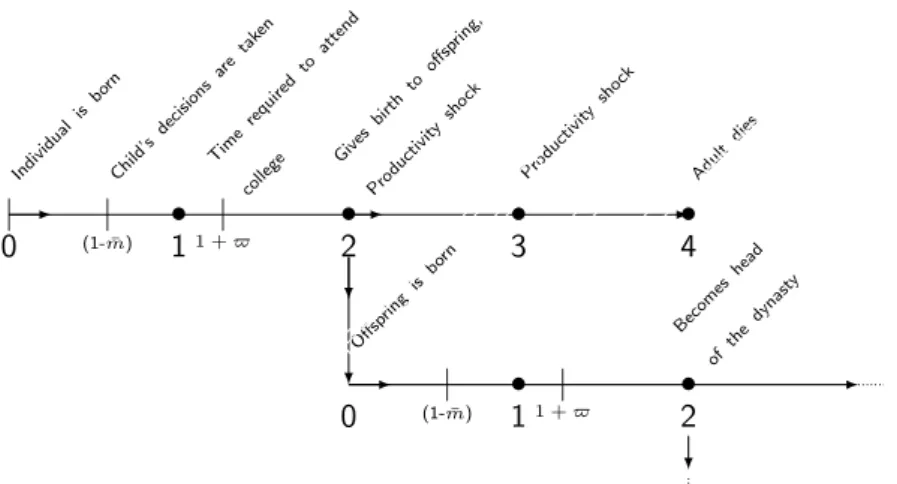
The economic environment consists of overlapping generations with discrete time and no population growth. Individuals live for four periods, one as a child, one as a young adult and two as adult parents. At the beginning of their third period of life, individuals give birth to a child. Thus, each household consists of an adult parent and either a child or a young adult. The dynasty is the relevant agent in this economy. Following Basu and Van (1998), we assume that all decisions are jointly taken within the dynasty, so there is no conflict among its members. Additionally, an individual dies at the end of the fourth period. Figure 1 provides a representation of the life cycle in this economy.
A model period consists of 17 years. However, during his first 9 years of life6, an
individual cannot work. During the other eight years, the child can work, go to school or allocate his time to leisure. It is possible to choose among three levels of schooling in this period: no schooling at all, only primary schooling, and secondary schooling. Schooling has not only explicit costs but also a cost in terms of time endowment, which also depends on the educational level chosen. A young parent of the same dynasty supplies all of his time (which is normalized to one) to the representative firm, in exchange for wages.
At the end of the first period of life, a child becomes a young adult and a young parent becomes an old parent. If a young adult has completed secondary schooling, he can choose to continue to college, which takes 4.5 years of his time time endowment and costs a certain amount of resources. The remainder of a young adult’s time is fully devoted to work (an old parent also devotes his full time endowment to work). At the end of this period, a young adult becomes a young parent as the old parent dies. In this way, the dynasty continues as generations overlap.
A dynasty can spend its resources on consumption, schooling or precautionary savings (which, in the second period, take the form of bequests). In this economy, there is is only one way to directly transfer resources over time, which is by lending to the representative firm. The representative firm faces no uncertainty, and thus, in the following period, always pays interest to its lenders.
6
Figure 1: The Life Cycle • • • • • • | | | | | 0 Indi vidu alis born
(1-m¯)
Child ’sde cisio ns are take n
11 +̟
Tim ere quire dto atte nd colle ge 2 Giv esbi rth to offsp ring, Prod uctiv ity shoc k 3 Prod uctiv ity shoc k 4 Adu ltdi es Offs prin gis born
0 1 2
Bec omes head ofth edy nast y
1 +̟
(1-m¯)
2.2
Preferences
We divide the dynasty’s life cycle into two periods. In the first period the dynasty consists of a child and a parent living through its third period of life. In the second, it consists of a young adult and an adult who is living through its fourth period of life.
Each dynasty seeks to maximize its discounted expected utility. In the first period, the utility function is:
u1(c, m) = log(c) +φlog(1−m) (1)
The first term of the r.h.s represents the perceived utility from household consumption,
while mrepresents the amount of time a children works, and φ >0 weights the utility
obtained from child leisure. Note that leisure and schooling time are perfect substitutes in the utility function. The reason is that we assume that households care about their
children’s education and leisure and dislike child labor7.
In the second period, there is no child labor decision. Hence, the dynasty utility function is simply represented by:
u2(c) = log(c) (2)
7
2.3
Age-Earnings Profile
The effective units of labor an individual can supply to the market are given by his productivity, which depends on his human capital level and on an exogenous shock.
There are four levels of human capital, hi ∈ {h0, h1, h2, h3}, which refer,
respec-tively, to no schooling8, primary schooling, secondary schooling and college education.
The total supply of labor efficiency units of an individual who is living through histth
period of life and whose level of human capital is h is given by zξ(t, h), where z is a
productivity shock.
Productivity shocks only affect adults. Letzi be a shock that affects the adult of a
household i. We assume thatzi follows a lognormal distribution.
log(z′i) =−(1−ρ)σ
2
2 +ρlog(zi) +ǫi, ǫi ∼N(0, σ
2), (3)
where ρ ∈ (0,1). Note that we normalize the unconditional average of this AR(1)
process to be−σ2
2 , so we haveE(z) = 1. There are two underlying assumptions behind
this exogenous process. First, the persistence of productivity is considered within
household, not within individuals. That is, the productivity of the parent who is living through his fourth period of life affects the productivity his son will have in the next period in the same way that the productivity of a parent living through his third period
of life affects his productivity during his last period of life9. Second, the productivity
variance is the same regardless of an individual’s age or education.
2.4
Production Technology
The representative firm has the usual constant returns to scale technology:
F(Kt, Lt) =AKtαL1t−α, (4)
whereKtdenotes the aggregate level of capital,Ltthe aggregate level of labor efficiency
units and Ais the TFP. All levels of human capital (including child labor) are perfect
substitutes (as in Basu and Van (1998)). The firm pays an interest rate r and wages
8
For calibration purposes, “no schooling” should be considered “incomplete primary schooling”. The reason is that, in the calibration procedure, we consider the share of the adult population that hascompleted each level of schooling (primary, secondary, and college). Therefore, the first level of human capital (h0)
includes individuals who did not complete primary schooling. See section 3.1 for more on this issue.
9
w for its inputs.
Since capital depreciates at rate δ, the firm’s problem becomes:
max {Kt,Lt}≥0
AKtαL1t−α−wLt−(r+δ)Kt (5)
The firm’s problem yields the following competitive labor and capital prices:
wt=A(1−α)
Kt
Lt
α
(6)
and
rt=Aα
Kt
Lt
α−1
−δ (7)
2.5
Schooling Technology
To invest in human capital accumulation, dynasties send their children and young
adults to school and college, respectively. We denote by κ(h) the cost of obtaining h
units of human capital.
Attending school also requires a fraction of an individual time endowment, which cannot be allocated to working. In the first period, this fraction is strictly increasing in the level of education. In the second period, young adults who attend college also
forgo a fixed fraction of their time endowment. We will use the function ς(·) and the
parameter̟to denote the time required to acquire a certain level of human capital10.
2.6
The Government
The government maintains a balanced budget in each period. Its revenues consist of
income taxes, denoted as τ. It rebates its revenues through conditional transfers,
sub-sidies, or both. The transfers may be conditioned on (i) school enrollment and (ii)
income thresholds. The transfer is denoted by η and I ∈ {0,1} denotes the eligibility
indicator. Finally, the government also determines a subsidy schedule, which is
repre-sented by the function S(h).
We assume throughout this paper that the government is fully credible and that its policies are fully observable. Hence,in a steady state equilibrium, policies are constant over time. We also assume that government policies are fully enforceable at no cost.
10
2.7
The State Space
The state space of a dynasty that is in the first period consists of the bequest it received
a, the human capital accumulated by the young adult h, and the productivity shock
that affects him z. Let the state space of period one be denoted by x1 ={z, h, a}.
For families that are living through the second period, the state space consists of
the parent’s level of human capital (still denoted byh), the education the young adult
has acquired in the first period, denoted byhc, the parent’s observable shock, and their
initial level of asset holdings are considered. We define the state space of the second
period dynasty as x2 ={z, h, hc, a}.
2.8
The Dynasty’s Recursive Problem
To begin, we’ll divide the dynasty’s problem into three parts. First, we follow the distinction made in section 2.2 and separate two periods of a dynasty: we denote period one as the period during which the parent is living through his third period of life and the child is living through his first period. Period two is defined as the period during which the head of the dynasty is going through his last period of life.
For simplicity, we also divide the dynasty’s problem in period two into two parts, depending on whether the dynasty’s young individual has completed secondary school.
2.8.1 Period 1
In the first period, the household’s problem can be defined as:
V1(x1) = max
c,m,h′,a′log(c) +φlog(1−m) +β
X
z′
Prob(z′|z)V2(z′, h, h′, a′) (8)
subject to:
0≤m+ς(h′)≤m¯ (9)
c+ (1− S(h′))κ(h′) +a′ =a+ (1−τ)[zξ(3, h)w+ra] +ξ(1, h′)mw+ηI (10)
h′ ∈ {h0, h1, h2} (11)
a′ ≥a (12)
where β is the discount rate, ¯m is the child’s available time endowment, a is an
ex-ogenous credit constraint, and I equals one if the household is eligible to receive the
transfer and 0 otherwise. Note that the argumenthreappears in the continuation value
of the dynasty, because the adult parent can no longer invest in education, and thus, his current level of human capital is carried into the next period.
Constraint (9) is the fraction of the child’s time that can be used to attend school and work (the remainder is implicitly allocated to leisure). Equation (10) represents
the dynasty’s resource constraint. On the right-hand-side, the expression [(zξ(3, h) +
ξ(1, h′)m)w] represents the gross labor income of the family - we assume that only the
adult wages are taxed. The term zξ(3, h) represents the efficiency units of labor
sup-plied by the adult parent, and ξ(1, h′) represents the efficiency units of labor supplied
by the child. On the left-hand-side, the term [(1− S(h′))κ(h′)] represents the net cost
of acquiring the level of human capital h′, a′ is the quantity of the assets that will be
carried into the next period, andc is consumption.
Constraint (11) represents the human capital investment possibilities in period 1, which are no schooling, primary, or secondary schooling, while equation (12) repre-sents the credit constraint. Finally, expressions (13) represent time feasibility and consumption non-negativity.
2.8.2 Period 2 - Dynasties whose children attended secondary school
In the second period, a household whose young adult has completed secondary schooling and can thus still attend college, solves:
V2,s(x2s) = max
c,g,a′log(c) +β
X
z′
Prob(z′|z)V1(z′, h′, a′) (14)
subject to:
g∈ {0,1} (15)
h′ =h3g+h2(1−g) (16)
c+g(1− S(h3))κ(h3) +a′ =
a+ (1−τ)[(zξ(4, h) +ξ(2, h2)(1−g) +g(1−̟)ξ(2, h3))w+ra] +ηI
(17)
c≥0, (19)
wherex2s= (z, h, h2, a),̟represents the time required to attend college, andgequals
one if the young adult attends college and 0 otherwise. As before, restrictions (18) and (19) refer to the credit constraint and to the non-negativity of consumption, respec-tively.
Equation (17) is the household’s resource constraint. On the left-hand-side, (1−
S(h3))κ(h3) is the net cost of attending college. On the right-hand-side, [(zξ(4, h) +
ξ(2, h2)(1−g)̟+g(1−̟)ξ(2, h3))w] is the total gross labor income of the dynasty,
zξ(4, h) is the efficiency units of labor supplied by the adult parent,ξ(2, h2) the total
labor efficiency units supplied by the young adult who does not attend college, and
ξ(2, h3) represents the efficiency units supplied by the young adult who attends college.
Notice that ξ(2, h3) will be supplied only during a fraction (1−̟) of a period.
2.8.3 Period 2 - Dynasties whose children did not attend secondary school
In the second period, the household whose young adult did not complete secondary schooling and thus cannot attend college solves:
V2,n(x2n) = max
c,a′ log(c) +β
X
z′
Prob(z′|z)V1(z′, h′, a′) (20)
subject to:
c+a′ =a+ (1−τ)[(zξ(4, h) +ξ(2, hc))w+ra] +ηI (21)
h′ =hc (22)
a′ ≥a (23)
c≥0, (24)
where x2n = (z, h, hc, a) and hc ∈ {h0, h1}, which, along with (22), states that the
2.9
Definition of Equilibrium
A stationary recursive competitive equilibrium consists of:
D1 Three groups of functions: (i) {V1, gc1, gh1, g1m, g1a}, (ii) {V2,n, g2c,n, ga2,n}, and (iii)
{V2,s, g2c,s, gh2,s, g2a,s} defined as follows:
i The value function, consumption, the human capital, child’s labor supply, and asset holdings policy functions, which all correspond to the first period.
ii The value function, consumption, and asset holdings policy functions, which all correspond to the second period when the young adult cannot attend college.
iii The value function, consumption, human capital (college), the asset holdings policy functions, which all correspond to the second period when the young adult has previously attended secondary school.
D2 Factor prices{w, r}.
D3 A government policy{τ,S(h), η} and an eligibility criterion.
D4 A pair of time-invariant measures over statesλ1 andλ2 that refer to periods one
and two, respectively, and whose laws of motion are:
λ2(z′, h, h′, a′) =
X
{(z,h,a):h′=gh
1,a′=g
a
1}
P rob(z′|z)λ1(z, h, a) (25)
and
λ1(z′, h′, a′) =I(hc < h2)
X
{(z,h,a):h′=hc,a′=ga
2,n}
P rob(z′|z)λ2(z, h, hc, a)
+
I(hc=h2)
X
{(z,h,a):h′=gh
2,s·h3+(1−g2h,s)·h2,a′=ga2,s}
P rob(z′|z)λ2(z, h, hc, a)
(26)
where,
1 Given [D2] and [D3], the group of functions [D1] maximize the household problems defined in the previous section.
3 The government operates with a balanced budget:
Γ = X
z,h,a
λ1(z, h, a)κ(g1h)· S(g1h) +
X
z,h,hc,a
λ2(z, h, hc, a)g2h,sκ(h3)S(h3)
+η
X
z,h,a
Iλ1+
X
z,h,hc,a Iλ2
,
(27)
where Γ represents the government revenues andI(eligibility) is a function of the
households’ states and choices. As child labor is not taxed:
Γ =τ(rK+wL)− X
z,h,a
h
ξ(1, g1h)mwi, (28)
whereL and K will be defined below.
4 Market clearing and consistency conditions hold:
X
z,h,a
λ1g1c+
I(hc < h2)
X
z,h,hc,a
λ2g2c,n
+
I(hc =h2)
X
z,h,hc,a
λ2gc2,s
=C, (29)
which is total consumption;
X
z,h,a
λ1κ(g1h) +
I(hc =h2)
X
z,h,hc,a
λ2κ(h3)·gh2,s
=E, (30)
which represents the total education expenditures;
X
z,h,a
λ1g1a+
I(hc< h2)
X
z,h,hc,a
λ2ga2,n
+
I(hc =h2)
X
z,h,hc,a
λ2ga2,s
=K, (31)
which represents the aggregate level of capital, and
X
z,h,a
λ1(ξ(3, h)zh+ξ(1, g1h)g1m) +
I(hc < h2)
X
z,h,hc,a
λ2(ξ(4, h)zh+ξ(2, hc)hc)
+
I(hc =h2)
X
z,h,hc,a
h
λ2(ξ(4, h)zh+ (1−g2h,s)ξ(2, h2)h2+gh2,s(1−̟)ξ(2, h3)h3)
i
=L,
(32)
which represents the aggregate level of labor supply measured in efficiency units. Finally, the resource constraint is:
3
Calibration
This section describes how we choose the model parameters and functions, which
in-clude A,a,β,α,δ,ξ(·), κ(·),ς,̟,σ2,ρ,S(·), andφ.
First, we normalizeA= 1. We also set the annual rate of depreciation to 0.06, as is
standard in the business cycles literature, so δ= 0.6507, and the borrowing constraint
toa= 0.
The time required to attend school is chosen as follows. First, we suppose that schooling takes one-half of the child’s non-sleeping daytime. Moreover, we assume that,
consistent with Brazilian legislation at the time11, the minimum number of school days
is 200. Dividing this number by the number of non-weekend days means that a child
must attend school over 75% of a year’s week days12.
In Brazil, secondary school lasted three years while primary lasted eight in 199713.
We assume that every child completes at least the third grade of primary school. Hence,
completing primary schooling requires 12·0.75·175 = 11%14of a child’s time endowment
in that period. Recall that the child’s effective time endowment in the first period is
only 178 , because we only have data for children 10 years or older. Likewise, attending
primary and secondary school requires 12 ·0.75·178 = 17%15 of a period’s time.
We also assume that college and work are mutually exclusive and that attending
college requires 4.5 years16. Hence, the young adult who chooses to attend college
works for the remaining time, which corresponds to 1217.5 = 73.5% of a period time
endowment.
3.1
Age-Earnings Profile
The data source used to estimate ξ(t, h) is the 1997 Pesquisa Nacional por Amostra
de Domic´ılios17. In order to calculate the age efficiency profile, we restrict the data to
11
Law 9394/96.
12
The same legislation states that these days should incorporateat least 800 hours of classes, excluding examinations. We also include other transaction costs, such as transportation and exam time, in the time required to attend school; thus, we found it reasonable to assume that schooling requires 50% of a child non-sleeping hours.
13
According to Law 11274/2006, the number of years of primary schooling increased to nine in 2010.
14
One-half of the child’s daytime multiplied by 75% of the year’s days for 5 of 17 years.
15
One-half of the child’s daytime multiplied by 75% of the year’s days for 8 of 17 years.
16
Restuccia and Urrutia (2004) assume that college takes 4 years while Bohacek and Kapicka (2012) assume that it takes 5 years.
17
white males who work 40-48 hours per week.
First, to obtain the values of ξ(1, h′), we need to take into account the dynasty’s
decision about the child education. For example, if a child only attends primary school and then works the remaining time, at the end of the period he will have worked part-time over five years with no investment in human capital and full part-time for three more years, after primary school is completed.
With this fact in mind, our hypothesis is that the (potentially) working child divides his labor hours proportionately to his available time in each condition. In the example above, the child’s labor efficiency corresponds to a weighted average of five years of working part time in addition to three years of working full time.
With regard to the remaining values of ξ(t, h), we take the average wages in each
age range, conditional on the educational level. We then normalize ξ(2, h0) = 1 and
calculate all other productivities relative to this value18.
Table 1: Age-earnings profile.
ξ h0 h1 h2 h3
t= 1 0.49 0.56 0.54
-t= 2 1 1.37 2.28 5.42
t= 3 1.41 2.3 4.12 7.94
t= 4 1.29 4.17 4.47 9.26
To calibrate the exogenous productivity process, we approximate a continuous
AR(1) process using ten grid points, following Tauchen (1986). To estimate σ, we
estimate a static log-wages regression, whose residual variance19equals σ2
1−ρ2. Thus, by
finding a value for ρ (see section 3.3), we are able to identify the value ofσ.
3.2
Fiscal Policy
In Brazil, schooling is heavily subsidized, at all levels. For instance, in 2000, public ex-penditures on education, including federal, state and municipality spending, accounted
It has been performed since 1967 on a nearly annual basis, with the exception of census years. In 1997, it surveyed 346,269 individuals out of an estimated population of 163,470,521.
18
In each human capital category, we only take into account the average wages of individuals who have
completedthat level of schooling. Therefore,h0 should be seen as “incomplete primary schooling”, rather
than “no schooling”.
19
for 3.9% of GDP20. In order to estimate the fraction of public education expenditures per student, we use information from two databases: the National Institute for Edu-cational Research and Policy (INEP) and the Brazilian household expenditures survey
(POF)21.
First, the INEP provides an estimate of public expenditures as a fraction of per capita GDP. We use the 2002 estimates, to match the data from the expenditures
survey. In 2002-2003, for each student in the fifth through eighth grades of primary
schooling (10-14 year olds), the expenditures per student corresponded to 12.3% of per capita GDP. The same ratio for secondary students was 8.9%, while for tertiary students it was 121%.
Given these ratios, we estimated the private expenditures in education per student. We use the 2002-2003 POF. For each family in this survey, we have information on education expenditures divided into six categories: (i) expenses for regular courses, which are defined as primary or secondary education expenses, (ii) expenses for ter-tiary education, (iii) total expenses for other courses, (iv) total expenditures on books and scientific publications, (v) total expenditures on school articles, and (vi) other expenses.
We then separate the families that spend exclusively on either college or regular courses. Therefore, we assume that a family that spends only for one category devotes all other education expenditures to activities or goods linked to that category, which are also considered education expenditures in our model. Finally, to assess the average expenditure per student, we assume that every family has two adults, and hence, we divide the average expenditures for each category by the average household size minus two. Finally, because we do not have separate data for primary and secondary educa-tion, we suppose that average private expenditures on both are the same.
Finally, we divide the estimated values by 2002 per capita GDP. We found that each tertiary education student has private costs of 32.9% of the per capita income, while a
student in a regular course costs, on average, 11.9%22. We use these values to estimate
the subsidy function, obtaining S(h1) = 53.4%, S(h2) = 50.0% andS(h3) = 54.73%.
20
Source: INEP/MEC
21
The Pesquisa do Or¸camento Familiar is a Brazilian household survey that gathers information about household expenditures on a wide range of items. In 2002, this survey included 48.470 households.
22
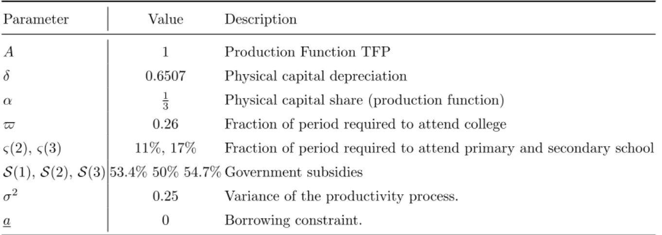
Table 2: Literature and Data Parameters.
Parameter Value Description
A 1 Production Function TFP
δ 0.6507 Physical capital depreciation
α 13 Physical capital share (production function)
̟ 0.26 Fraction of period required to attend college
ς(2),ς(3) 11%, 17% Fraction of period required to attend primary and secondary school
S(1), S(2),S(3) 53.4% 50% 54.7% Government subsidies
σ2
0.25 Variance of the productivity process.
a 0 Borrowing constraint.
3.3
Simulated Method of Moments
Thus far, we have estimated 26 parameters (some of which are part of the same func-tions) from the literature or using Brazilian data. The remaining six parameters are jointly calibrated using the model to simulate a set of six exactly identified empirical moments. Let the parameter vector be:
Θ = [φ κ(h1) κ(h2) κ(h3) β ρ]′ (34)
The model generates six moments, which are denoted by M(Θ). The vector of targets
is denoted byMs and summarized in table 3. We find the estimate for ˆΘ by:
ˆ
Θ = arg min Θ
[M(Θ)]−Ms]′W[M(Θ)−Ms] (35)
where W is a weighting matrix. Here, we set W =I, because there is no clear choice
of W.
As for the targets, we choose statistics that have a direct relationship with each
identified parameter. Initially, we identifyφ, the parameter that governs the preference
for child labor, using PNAD data for the share of children between 10 and 17 years
old who were working. To identify the costs of schooling (κ(·)) we match the shares
of the population that have completed each educational level, taking into account only
individuals who were 25 to 34 years old. To identifyβ in this model, we use Brazilian
gross fixed capital formation, taking the average from 1992 to 2002. Finally,ρ is
Table 3: Empirical Moments.
Ms,i Model Data Description
i=1. 22.05% 21.95% Fraction of children who work (PNAD 1997).
2. 18.81% 19.22% Fraction of adults who completed only primary education (PNAD 1997). 3. 25.39% 24.92% Fraction of adults with secondary education but not college (PNAD 1997). 4. 8.39% 7.78% Fraction of adults who completed tertiary education (PNAD 1997). 5. 17.71% 17.86% Gross capital formation (IBGE)
6. 0.69 0.69 Intergenerational elasticity of earnings (Dunn (2007))
Table 4: Parameters Obtained through the Simulated Method of Moments.
Parameter Value Description
φ 1.13 Marginal disutility of child labor.
κ(h1) 0.66 Gross cost of primary schooling.
κ(h2) 1.60 Gross costs of obtaining both primary and secondary schooling.
κ(h3) 6.61 Gross costs of college education.
β171 0.97 Preference rate of discount (annual).
ρ 0.66 Persistence of the exogenous productivity shock process.
4
Results
4.1
Benchmark Policy
We construct the transfer schedule for our benchmark policy by defining a basic trans-fer and a basic income threshold. The basic income threshold includes net capital and net labor earnings, but excludes child labor earnings. The basic transfer is treated as a
normalization, and corresponds to what an extremely poor23family would receive if its
children finished secondary schooling. All other transfers are proportional to the basic transfer, and we use the same ratios defined by the Brazilian Ministry of Social
Devel-opment for theBolsa Fam´ıliaProgram in 2013. Every household whose income is below
the basic threshold that complies with the schooling requirement receives a transfer (in the case of attending only primary school, 5/8 of the basic transfer). Moreover, every household whose earnings are less than two times the basic threshold receives another
23
transfer, also conditional on schooling, as doBolsa Fam´ılia beneficiaries. The transfer schedule is summarized in table 5. We then set the basic transfer and thresholds such that, in the new steady state equilibrium, the program’s total budget corresponds to 0.55% of total output and the program’s coverage corresponds to 20.7% of families,
following the 2013 figures for Bolsa Fam´ılia.
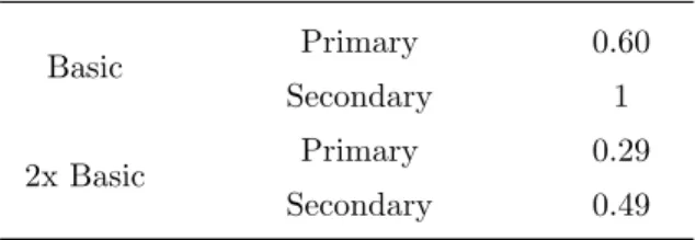
Table 5: Summary of the Transfer Policy
Threshold Schooling Conditionality Transfer
Basic Primary 0.60 Secondary 1
2x Basic Primary 0.29 Secondary 0.49
Note: The values displayed in the third column corre-spond to the total transfer received, relative to the trans-fer received by families below the basic threshold and whose children complete secondary schooling.
Due to the policy design, it is possible that some mistargeting occurs. Mistargeting, in the context of this model, happens when a family whose income is below the threshold does not receive the transfer for some reason. In this model, mistargeting occurs if the transfer is so small that it does not compel a family to bear schooling costs, so the
family optimally decides not to accept the transfer. Because we have set a transfer
coverage goal of 20.7%, the existence of mistargeting means that the very poorest families do not receive the transfer, but some middle income families do. In fact, in the post-CCT steady state equilibrium, 19% of the families that are eligible choose not to accept the transfer. This number is not insignificant, but it is below existing estimates
for the Bolsa Fam´ılia program (see Soares et al. (2009)). In section 4.5 we consider an
experiment in which mistargeting is not a concern.
4.2
Long Run Results
The most notable influence, by far, of the Bolsa Fam´ılia program is on human capital
schooling dramatically increases from 19% to nearly 50%, while the share of the adult population that has completed up to secondary school increases from 25% to 32%. Finally, there is virtually no modification on the tertiary enrollment rate. In fact, be-cause the families whose young adults enter college are among the richest ones (their average incomes are nearly four times the per capita income and ten times greater than the average income of the transfer beneficiaries), the new policy can only affect their decision through general equilibrium effects. For instance, wealthier families maybe benefit from higher interest rates (see table 7). However, equilibrium effects are not so strong, as they only cause a slight increase in tertiary school enrollment (by 5% or 0.45 percentage points).
The new policy’s impacts on human capital accumulation can be explained by two
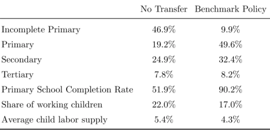
Table 6: Educational and Child Labor Outcomes (Long Run)
No Transfer Benchmark Policy
Incomplete Primary 46.9% 9.9% Primary 19.2% 49.6% Secondary 24.9% 32.4% Tertiary 7.8% 8.2% Primary School Completion Rate 51.9% 90.2% Share of working children 22.0% 17.0% Average child labor supply 5.4% 4.3%
mechanisms: direct and indirect. First, the transfer directly affects school enrollment through its eligibility requirements. By itself, this channel is responsible for the largest share of the increase in human capital accumulation - the school eligibility requirement induces the vast majority of children to complete at least primary school. Second, the direct impact on workforce quality increases the marginal return to physical capital and thus induces its accumulation. A higher level of physical capital implies that a given quantity of working hours is able to produce more, which in turn encourages more investment in human capital. In fact, this indirect effect is responsible for the
majority of the increase in secondary schooling investment24.
Over the long run, increased human capital accumulation has important macroe-conomic impacts, as shown in table 7. The aggregate labor efficiency units increase
24
by 22%, while the aggregate physical capital increases by 15.6%, resulting in a nearly 20% increase in per capita output.
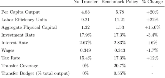
Table 7: Macroeconomic Indicators
No Transfer Benchmark Policy % Change
Per Capita Output 4.83 5.78 +20% Labor Efficiency Units 9.21 11.21 +22% Aggregate Physical Capital 1.32 1.53 +15.6% Investment Rate 17.9% 17.3% -3.4% Interest Rate 2.67% 2.83% +6% Wages 0.349 0.343 -1.7% Tax Rate 15.4% 17.3% +12% Transfer Coverage 0% 20.7% -Transfer Budget (% total output) 0% 0.55%
-To understand the magnitude of these results, we examine the incentives to accumulate physical capital. The conditional transfer serves as insurance, weakening precautionary
motives, even for families whoare not eligible. This happens because every household
in the economy has a chance of being affected by a series of negative productivity shocks leading to poverty. As a result, all else equal, every family has some incentive to save less. However, the schooling requirements are able to fully offset the perverse effects implied by weakened precautionary motives. For the sake of comparison, if we
kept the transfer schedule but eliminated any schooling requirement25, the new total
labor efficiency units in the steady state would decrease by 17.5%, compared with a 22% increase in the proposed schedule. This difference illustrates the importance of introducing schooling requirements along with a conditional cash transfer policy. As workforce quality increases, the marginal return on physical capital increases, encour-aging investment in education, increasing the marginal return on physical capital, and thus increasing physical capital accumulation.
25
Higher workforce quality has a direct effect on child labor. The larger share of parents with higher education and, thus, higher labor incomes, means that there is less need for child labor, as shown in table 6. The share of working children decreases from 22% to 17% and total child working hours decrease by 20%. However, one-half of working children also complete primary schooling, contrary to the non-CCT case, wherein the share of children who work and complete any schooling was less than 1%. Over the long run, we observe a decrease in net wages, due to higher taxes and the increase in the supply of labor efficiency units. In fact, this could be the driving force of the observed reduction in child labor supply, rather than the human capital accu-mulation channel. To evaluate the magnitude of the wage reduction effect over child labor, we simulated a version of the model where we provided the same transfer sched-ule but held the (gross) wages constant at the pre-CCT level, which is higher than the post-CCT equilibrium wages. The share of working children was 16.1%, showing that
higher wages actually reduced child labor. The reason is that higher wages increased
household income overall, alleviating the need for child labor. Therefore, we infer that human capital accumulation is indeed the driving force reducing the share of working children.
4.2.1 Poverty and Inequality
Child labor and education are directly related to poverty, and one of the main goals of the Bolsa Fam´ılia program is precisely to reduce poverty. So far, we have observed that the Bolsa Fam´ılia effectively increases schooling and reduces child labor over the long run. We now evaluate the program’s performance regarding poverty and inequality, which is presented in table 8. We define the poverty line based on the income dis-tribution generated by the model. In 1997, the Brazilian headcount ratio was 20.5%, according to the World Bank. We then set the poverty line to correspond to the 20.5 quantile of the income distribution of the calibrated pre-CCT model.
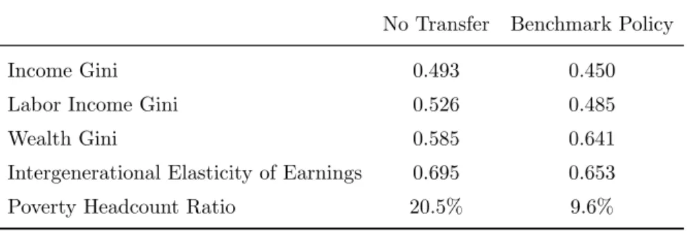
The CCT policy is able to reduce poverty by 10.9 percentage points from the bench-mark, from 20.5% to 9.6%, which represents a 53% decrease. The driving force here is human capital accumulation, a fact that will become even clearer when we analyze the transition. Additionally, there is a decrease in the degree of persistent of earnings, as the intergenerational elasticity of labor earnings falls from 0.695 to 0.653. Thus, in the long run, our results suggest that conditional cash transfers are effective in improving social mobility
Table 8: Poverty and Inequality Outcomes
No Transfer Benchmark Policy
Income Gini 0.493 0.450 Labor Income Gini 0.526 0.485 Wealth Gini 0.585 0.641 Intergenerational Elasticity of Earnings 0.695 0.653 Poverty Headcount Ratio 20.5% 9.6%
result differs from Cespedes (2010), who predicts that the long-term effects of the Mexican PROGRESA program on inequality are small. A possible explanation is that
Bolsa Fam´ılia represents 0.55% of Brazilian output, while in contrast PROGRESA represents only 0.1% of Mexican output. Finally, it is interesting to see that wealth inequality is exacerbated by the new policy. This fact is due to the asymmetric dis-tortion of precautionary motives implied by the conditional cash transfer. Specifically,
because there is a positive correlation between asset holdings and total income26, less
wealthy families are relatively more insured than richer ones. This asymmetry causes the poorest families to reduce their savings relatively more than the wealthy, which aggravates wealth inequality.
4.3
Transitional Dynamics
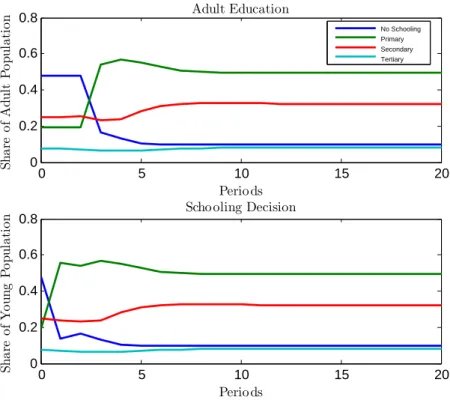
In this section, we evaluate the transitional dynamics between the pre-CCT equilibrium and the post-CCT equilibrium. We start by looking at the human capital accumula-tion dynamics (figure 2). First, note that there is an immediate sharp increase in the share of children that complete up to primary school, from 19% to 54%. However, this increase is not accompanied by secondary enrollment, which even slightly decreases at the beginning of the transition. To understand why this happens, we must examine the price movements (figure 3).
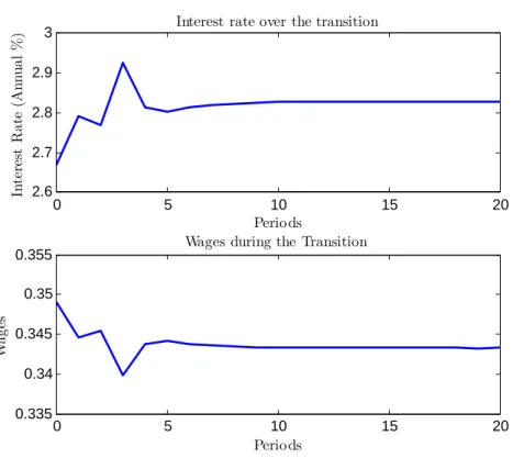
In the first period of the transition, the relative return on human capital invest-ment falls remarkably as wages decrease and the interest rate rises. Because the labor supply (measured in efficiency units) remains constant over the short run (see figure 4), we conclude that the weakened precautionary motives drive this price movement. The reduction of the investment rate corroborates our conclusion (figure 5). There
26
Figure 2: Evolution of Education
0 5 10 15 20
0 0.2 0.4 0.6 0.8 Periods S h a re o f Ad u lt P o p u la ti o
n Adult Education
No Schooling Primary Secondary
Tertiary
0 5 10 15 20
0 0.2 0.4 0.6
0.8 Schooling Decision
Periods S h a re o f Y o u n g P o p u la ti o n
Note: The top graphic displays the share of the adult population that has completed (up to) a certain level of education. The bottom graphic displays the share of the young population that completes a certain level of schooling.
is an overall disincentive to education over the short run, especially in the first and second periods of transition. On the other hand, the conditional transfer also provides an incentive to increase schooling, although only for targeted families. Because the schooling requirements of the transfer policy in the first period are only sufficient to induce households to enroll their children in primary school, secondary school attain-ment decreases.
Figure 3: Evolution of Wages and Interest Rates
0 5 10 15 20
2.6 2.7 2.8 2.9
3 Interest rate over the transition
Periods
In
te
re
st
R
a
te
(An
n
u
a
l
%
)
0 5 10 15 20
0.335 0.34 0.345 0.35
0.355 Wages during the Transition
Periods
W
a
g
es
During the fourth period of the intervention, the growth of physical capital stock not only reduces interest rates but also reverses the downward wage trend, attracting investments in human capital. It is also at that point that investments in secondary and tertiary schooling begin to increase, giving a final boost to physical capital ac-cumulation. The complementarity between human and physical capital accumulation continues to take place during the smooth convergence to the new steady state equi-librium.
The dynamics described above emphasize the role of a general equilibrium approach to evaluating the impacts of a conditional cash transfer. Price movements play a cru-cial role during the first periods of the intervention, but diminish until convergence. As a result, the interest rate is higher than before, but it remains much lower than its peak during the third period of intervention. However, wages remain lower than in the pre-CCT steady state, and not far from their lowest value during the transition.
Figure 4: Evolution of Macroeconomic Variables
0 5 10 15 20
9 9.5 10 10.5 11
11.5 Aggregate Labor Efficiency Units
Periods
L
a
b
o
u
r
E
ffi
ci
en
cy
Un
it
s
0 5 10 15 20
1.3 1.4 1.5
1.6 Aggregate Physical Capital
Periods
P
h
y
si
ca
l
C
a
p
it
a
l
extensive (from 22% to 23%) and intensive margins (an increase of 26% of total hours supplied). This pattern persists during the second period, reversing only after three intervention periods. The transitional dynamics concerning child labor are displayed in figure 6.
During the first two periods of the transition, the majority of parents do not have sufficient income to pay for schooling, even with the conditional transfer. There-fore, families whose income is below the basic threshold find it optimal to receive the transfer and, at the same time, increase their child labor supply to pay the schooling costs. Moreover, there are some families (approximately 21% of eligible households in the first transition period) whose income is below the basic threshold but choose not to accept the transfer. As a result, these families become even more impoverished as taxes increase and wages decrease, increasing their need for child labor.
Figure 5: Evolution of Macroeconomic Variables (II)
0 5 10 15 20
4.5 5 5.5
6 Output during Transition
Periods
O
u
tp
u
t
0 5 10 15 20
0.16 0.17 0.18 0.19 0.2
0.21 Investment Rate
Periods
In
v
es
tm
en
t
(%
o
f
G
D
P
)
subsidies and transfers, decrease. Second, the new generation of adults is more edu-cated, which, along with increasing wages, provides higher labor income and alleviates poverty. Finally, the number of mistargeted families (those who decide not to accept the transfer) falls to its steady state value (19%), as the most impoverished families are increasingly able to comply with the schooling eligibility. Subsequently, the poorest families are less deprived as before, which reduces their need for child labor.
By the end of the transition, the level of child labor supply reaches its lowest, as
only 17% of children work. Therefore, our results suggest that the impact of Bolsa
Fam´ılia on child labor occurs mostly through its long-term general equilibrium effects. The fact that a conditional cash transfer, over the short run, is inefficient in address-ing child labor is already documented (see Cardoso and Souza (2004) and Rocha and Soares (2009)). Thus, we provide a possible explanation for that fact: Families need child labor in order to be able to afford schooling costs. However, as new generations of educated children become adults, labor income increases overall and child labor is no longer necessary.
Figure 6: Evolution of Child Labor
0 5 10 15 20
0.16 0.18 0.2 0.22
0.24 Total Child Labor
Periods
S
h
a
re
o
f
w
o
rk
in
g
ch
il
d
re
n
0 5 10 15 20
0.02 0.025 0.03 0.035
0.04 Total Child Labor Supply (Share of Available Time)
Periods
W
o
rk
in
g
Ho
u
rs
and inequality outcomes (figures 7 and 8). The Gini coefficient of labor income remains constant during the first period of transition, which is consistent with the existing
data27. However, if we consider the Gini coefficient on total earnings (which includes
capital rents and conditional transfers) we observe a reduction of 1.4 points. The
re-duction is fully driven by the transfer, because the Gini coefficient of capital income also remains constant over the short run. When the generation born in the first year of the intervention reaches adulthood, inequality is sharply reduced, and the new steady state income distribution is reached within one generation. With regard to poverty, the effects of the new policy arise during the first period of intervention. Therefore, the policy is able to alleviate poverty both directly - through the transfer itself - and indirectly - through the incentives to increase human capital accumulation.
27
Figure 7: Evolution of Inequality
0 2 4 6 8 10 12 14 16 18 20
0.46 0.48 0.5 0.52 0.54 0.56
Periods
Gini coefficient of Labour income
0 2 4 6 8 10 12 14 16 18 20
0.4 0.42 0.44 0.46 0.48 0.5
Periods
Gini coefficient of Total income
4.4
Welfare Evaluation
In this section we evaluate the impacts of the transfer policy on welfare. We measure welfare in terms of consumption equivalent units, as is usual in the literature. Let
Wi(xi) be the period i consumption equivalent welfare of a household whose state is
xi. So:
W1(x1) = 1
1−β [logg
c
1+φlog(1−gm1 )] , (36)
for the first period and
W2(x2) =
1
1−β logg
c
2, (37)
for the second period, where that g1c and gc2 are the consumption policy functions,
while gm
1 is the policy function for child labor supply. To obtain the total welfare of
the economy we simply integrate over the possible states, using the invariant measure
The results are shown in column (2) of table 9. Only 33% of individuals are better off immediately after the introduction of the policy, while total welfare decreases by 2.26%. This result is driven by the burdens imposed by higher taxes, lower wages, and reduced incentives for physical capital accumulation during the first years of the
transition28. Over the long run, however, as individuals become more educated and
thus increase their labor earnings, the initially heavy burdens translate into massive welfare gains (18.7%). Therefore, the transfer policy imposes a burden on the current generation in exchange for large welfare gains in the future, as we could expect from the long-term results presented in section 4.2.
28
If we compute the average welfare gains by asset holdings level, we see that those who hold no assets at all and those who hold a medium-level amount of assets (say, the middle class) are the segments of the population that mostly dislike the new policy. These are precisely the households that rely on labor income butdo notreceive transfers. The very poorest households choose not to receive the transfer because it would require school enrollment, which imposes costs that surpass the transfer benefits.
Figure 8: Evolution of the Poverty Headcount Ratio
0 5 10 15 20
8 10 12 14 16 18 20 22
Periods
He
a
d
co
u
n
t
R
a
ti
o
(%
Table 9: Welfare Analysis
Benchmark Policy
% better-off 33% % targeted better-off 87% Total Welfare -2.26% Total Welfare in new SS +18.7%
Note: Welfare is measured in consumption equivalent units. The first row presents the percentage of the entire population that is better off immediately after the intro-duction of the policy (in comparison to the steady state where no conditional cash transfer policy takes place). The second row presents the share of households who receive the transferduring the first period of transition that are better off right after the changing. The third row presents the total welfare modification right after the initiation of the new policy. The fourth row presents the total welfare modification after achieving the new steady state.
4.5
Counterfactual Experiment
In the last section, we have observed that the introduction of a conditional cash transfer
policy similar toBolsa Fam´ılia creates vast benefits in the long run, increasing human
and physical capital accumulation, while reducing child labor, poverty and inequality. However, in the short run, a large share of the population is hurt by higher taxes, lower wages and decreased incentives to accumulate physical capital. Based on this scenario, a natural question arises: could we provide a similar transfer scheme that maintains these long-term benefits while reducing the short-term costs?
Thus, we introduce a new policy that maintains the previous thresholds and trans-fers and introduces an extra transfer that does not require school enrollment and is
provided to any29 household whose total net earnings are below the basic threshold.
The extra transfer corresponds to 50% of the basic transfer.
In the long run, the effects are similar to the benchmark policy, but slightly weaker. This fact can be attributed both to the relatively lower incentive to schooling and to
29
the relatively higher insurance promoted by the transfer that does not require school enrollment. The impacts on educational attainment and child labor are presented in table 10. The transfer raises primary school completion to 83% and reduce the share of working children to 18%. In addition, the macroeconomic impacts of this policy are
quite similar to the benchmark case30, as are the results regarding inequality, which
are displayed on table 11.
In the short run, however, there are important differences with respect to the
Table 10: Educational and Child Labor Outcomes (Long Run) - Counterfactual Policy
No Transfer Counterfactual Policy
Incomplete Primary 46.9% 16.9% Primary 19.2% 45.6% Secondary 24.9% 29.8% Tertiary 7.8% 7.7% Primary School Completion Rate 51.9% 83.1% Share of working children 22.0% 18.0% Average child labor supply 5.4% 4.0%
Table 11: Poverty and Inequality Outcomes - Counterfactual Policy
No Transfer Counterfactual Policy
Income Gini 0.493 0.460 Labor Income Gini 0.526 0.485 Wealth Gini 0.585 0.664 Intergenerational Elasticity of Earnings 0.695 0.628 Poverty Headcount ratio 20.5% 10.8%
previous case. Figure 9 shows that the share of working children falls monotonically
towards the new steady state, with a 1.5 percentage point decrease in the first year of
30
the transition. This fall cannot be explained by differences in price movements, which
essentially follow the same path as in the benchmark policy31.
In fact, because the transfer is able to reach everyone below the threshold
regard-Figure 9: Evolution of Child labor - Counterfactual Policy
0 5 10 15 20
0.16 0.18 0.2
0.22 Total Child Labour
Periods
S
h
a
re
o
f
w
o
rk
in
g
ch
il
d
re
n
0 5 10 15 20
0.015 0.02 0.025
0.03 Total child labour supply (share of available time)
Periods
W
o
rk
in
g
Ho
u
rs
less of school enrollment, the very poorest also have a slight increase in their income,
contrary to what happened in the previous case. This leads to immediate poverty re-duction, which discourages child labor right after the intervention. This result suggests that a policy that prescribes a transfer and does not require school enrollment end up being effective in tackling child labor in the short run.
Finally, we examine the welfare impacts of the counterfactual policy. In the counter-factual intervention, 60% of households are better off, with 99% of targeted households benefiting from the new policy, and total welfare increasing by 3.86% immediately after the intervention. The increase in the share of households that are better off is because the new transfer is able to reach, right after its introduction, many households that
31
were not covered in the benchmark specification, including families whose members are only adults (young and old).
In the long run, however, total welfare only increases by 14.5%. This result shows that, as the economy gets richer, it is preferable, from a welfare point of view, to have a transfer program that requires school enrollment. In fact, we observe a trade-off between short-term and long-term welfare. In the counterfactual experiment, a trans-fer that was less strict in terms of conditionalities achieved less long-term benefits, in exchange for less welfare costs (in fact more welfare gains). On the other hand, the the “stricter” schedule achieves more long-term benefits, but at a high (welfare) cost to most households.
5
Conclusion
In this paper, we evaluate the long-term effects of conditional cash transfer programs,
such as the Brazilian Bolsa Fam´ılia, on human capital accumulation and child labor.
In the long run, we find out that a transfer policy that mimics theBolsa Fam´ıliais able
to sharply increase school enrollment and reduce the share of working children. School attainment rose significantly in the primary level, whose completion rate reaches 90% in the long run, as opposed to a previous 53% rate. On the other hand, the program had a smaller effect on secondary school completion (32.7% to 40.6%) and almost no effect on college attainment. The observed impact on child labor is more modest, al-though far from insignificant - the share of working children decreased from 22% to 17%.
By computing the transition to the new steady state, we are able to both evaluate the short-term welfare impacts stress the importance of considering general equilibrium effects in the analysis. Wage and interest rate movements have substantial impacts over the short run, affecting physical and human capital accumulation, and even increasing
child labor. This result suggests that the benefits ofBolsa Fam´ılia with regard to child
labor are still forthcoming. Additionally, we show that, in the mid-run, the incentives to schooling provided by the transfer are able to overcome the weakened precautionary motives implied by the conditional transfer. As a result, most of the benefits of the new policy are felt within the time gap corresponding to one generation.
that the transfer represents only 0.55% of the total output. All in all, we show that
Bolsa Fam´ılia can be a strong poverty alleviating policy that does not only benefit the targeted families, but is also able increase welfare and boost per capita income in the long run.
References
Barros, R. P. d., M. CARVALHO, S. FRANCO, and R. MENDONC¸ A (2006). Recente
da Desigualdade de Renda no Brasil. In: BARROS, R. P. de; FOGUEL, M. N.; ULYSSEA, G. Desigualdade de Renda no Brasil: Uma An´alise da Queda Recente., Volume 1.
Barros, R. P. d., M. Carvalho, S. Franco, R. Mendon¸ca, and R. A. (2010). Sobre a evolu¸c˜ao recente da pobreza e da desigualdade no brasil. Mimeo.
Basu, K. and P. H. Van (1998). The economics of child labor. The American Economic
Review 88(3), pp. 412–427.
Bohacek, R. and M. Kapicka (2012). A quantitative analysis of educational reforms in
a dynastic framework. Manuscript, University of California Santa Barbara.
Bourguignon, F., F. H. G. Ferreira, and P. G. Leite (2003). Conditional Cash Transfers, Schooling and Child Labor : Micro-Simulating Bolsa Escola. Technical report.
Cardoso, E. and A. P. Souza (2004, April). The Impact of Cash Transfers on Child La-bor and School Attendance in Brazil. Technical Report 0407, Vanderbilt University Department of Economics.
Cespedes, N. (2010, February). General equilibrium analysis of conditional cash trans-fers. Tecnhical report.
Chioda, L., J. M. P. de Mello, and R. R. Soares (2012, February). Spillovers from Conditional Cash Transfer Programs: Bolsa Fam´ılia and Crime in Urban Brazil. IZA Discussion Papers 6371, Institute for the Study of Labor (IZA).
Dunn, C. E. (2007). The intergenerational transmission of lifetime earnings: Evidence
from brazil. The BE Journal of Economic Analysis & Policy 7(2).
in Costa Rica. Research Department Publications 4359, Inter-American Develop-ment Bank, Research DepartDevelop-ment.
Erosa, A., T. Koreshkova, and D. Restuccia (2010). How Important Is Human Capital?
A Quantitative Theory Assessment of World Income Inequality. Review of Economic
Studies 77(4), 1421–1449.
Fiszbein, A., N. Schady, F. H. Ferreira, M. Grosh, N. Keleher, P. Olinto, and E. Skoufias
(2009, March). Conditional Cash Transfers : Reducing Present and Future Poverty.
Number 2597 in World Bank Publications. The World Bank.
Krueger, D. and J. T. Donohue (2004, March). On the Distributional Consequences of Child Labor Legislation. NBER Working Papers 10347, National Bureau of Eco-nomic Research, Inc.
Lichand, G. (2010, November). Decomposing the Effects of CCTs on Entrepreneurship.
World Bank - Economic Premise (41), 1–4.
Medeiros, M., T. Britto, and F. V. Soares (2008, June). Targeted Cash Transfer Pro-grammes in Brazil: BPC and the Bolsa Familia. Working Papers 46, International Policy Centre for Inclusive Growth.
Restuccia, D. and C. Urrutia (2004, December). Intergenerational Persistence of
Earn-ings: The Role of Early and College Education. American Economic Review 94(5),
1354–1378.
Restuccia, D. and G. Vandenbroucke (2008, October). The Evolution of Education: A Macroeconomic Analysis. Working Papers tecipa-339, University of Toronto, De-partment of Economics.
Rocha, R. and R. R. Soares (2009, April). Evaluating the Impact of Community-Based Health Interventions: Evidence from Brazil’s Family Health Program. IZA Discussion Papers 4119, Institute for the Study of Labor (IZA).
Soares, S., R. P. Ribas, and F. V. Soares (2009). Focaliza¸c˜ao e cobertura do programa bolsa-fam´ılia: qual o significado dos 11 milh˜oes de fam´ılias? Technical report, Texto
para Discuss˜ao, Instituto de Pesquisa Econˆomica Aplicada (IPEA).
Soares, S. and N. S´atiro (2009). O programa bolsa fam´ılia: Desenho institucional,