Effects on school enrollment and performance of a conditional transfers program in Mexico

,

~I;.,

. .

.

>-, ~ "~ ,

P/EPGE SPE

FUNDAÇÃO GETULIO VARGAS

'-0

FGV

EPOE

SEMINÁRIOS DE PESQUISA

ECONÔMICA DA EPGE

Effects on school enrollment and

performance of a conditional transfers

program in Mexico

PIERRE DUBOIS

(Université de Toulouse)

Data: 29/01/2004 (Quinta-feira)

Horário: 16h

Local:

Praia de Botafogo, 190 - 11

0

_andar

Auditório nO 1

Coordenação:

Effects on School Enrollment and Performance of

a

Conditional Transfers Program in Mexico

Pierre Dubois*, Alain de Janvry! Elisabeth Sadoulet

t

First Version: July 2000, This Version: April 2003+

Abstract

We study the effects of a conditional transfers program on school enrollment and perfor-mance in Mexico. We provide a theoretical framework for analyzing the dynamic educational decision and process inc1uding the endogeneity and uncertainty of performance (passing grades) and the effect of a conditional cash transfer program for children enrolled at school. Careful identification of the program impact on this model is studied. This framework is used to study the Mexican social program Progresa in which a randomized experiment has been implemented and allows us to identify the effect of the conditional cash transfer program on enrollment and performance at school. Using the mIes of the conditional program, we can explain the different incentive effects provided. We also derive the formal identifying assumptions needed to provide consistent estimates of the average treatment effects on enrollment and performance at school. We estimate empirically these effects and find that Progresa had always a positive impact on school continuation whereas for performance it had a positive impact at primary school but a negative one at secondary school, a possible consequence of disincentives due to the program termination after the third year of secondary school.

Key words: education demand, schooling decisions, school performance, dynamic decisions, treatment effects, transfer program, randomized experiment, Mexico.

JEL Classification: C14, C25, D91, H52, H53, 121, 128, J24.

'Corresponding author:

University of Toulouse (INRA, IDEI) Manufacture des Tabacs

21 allée de Brienne 31000 Toulouse France d ubois@toulouse.inra.fr

tUniversity of California, Berkeley.

c

-1

Introduction

In 1998, the Education, Health, and Nutrition Program, known by its Spanish acronym as Pro-gresa 1, was introduced in rural Mexico. The purpose of the program is to provi de resources and incentives to increase the human capital of the children of poor rural households, thus attempting to break the inter-generational inheritance of poverty. The program provides cash transfers as well as in kind health benefits and nutritional supplements to poor households, conditional on the child's school attendance and on regular visits to health centers. On average, these cash transfers represent 22% of the income of beneficiary families. The program has grown rapidly and was cov-ering 2.6 million rural families in extreme poverty in 2000, corresponding to about 40 percent of all rural families in Mexico. Progresa operates in 50,000 localities in 31 states, with a budget of approximately one billion dollars for 2000.

In Mexican rural communities, children tend to begin their labor force participation at early ages in order to contribute to family income. One of the main objectives of Progresa is to reduce this early labor force participation of children and thereby increase their enrollment and attendance at school. The program is made up of three closely linked components, education, health, and nutrition based on the idea that positive interactions between these three components enhance the effectiveness of an integrated program over and above the separate benefits from each of these components. The educational component of Progresa provides monetary educational grants conditional upon attendance at school and constitutes the main part of monetary benefits.

The purpose of this paper is to evaluate the impact of Progresa on the educational behavior of children. We develop a dynamic education demand model incorporating incentive effects of the edu-cational system on the behavior of students. The model incorporates the eduedu-cational grants system introduced by Progresa and shows that such a program does not only affect enrollment decisions but also behavior at school in terms of incentives to pass to higher grades, a crucial point which is not addressed in most education demand models. The most recent developments of education de-mand models embody the dynamics and uncertainty associated with wages and returns to schooling as well as liquidity constraints (De Vreyer, Lambert, Magnac, 1999; Magnac and Thesmar 2002a, 2002b; Cameron and Heckman, 1998, 2001; Cameron and Taber, 2000; Rosenzweig and Wolpin 1996; Eckstein and Wolpin, 1999, Keane and Wolpin, 1997, 2001). But, most models assume that schooling decisions allow households to choose with certainty the leveI of school attainment reached by each child or at least that the decision to continue revised each year does not involve any un-certainty in grade progression. Once the decision to enroll at school has been taken, the previous

1 Programa de Educación, Salud y Alimentación.

,

literature assumes that the child will pass the grade and benefit from the expected return of one additional year of schooling. This issue is addressed in Magnac and Thesmar (2002a) where grade completion is stochastic. They show in an application to France that one of the reasons for the rise in educationallevels observed in France between 1980 and 1993 is the decreasing selectivity of the education system. Cameron and Heckman (1998) model the transitions from one grade to the next as random processes depending on a number of characteristics without distinguishing whether non progression comes from school drop out or repetition. To our knowledge, there is no theoretical model where both the endogeneity and uncertainty in successfully passing grades are explicitly modelled. Here, we want to explicitly take these features into account because both school enroll-ment and school performance determine educational attainenroll-ment and the true developenroll-ment value of education. Understanding the determinants of school performance is particularly important in our case because the repetition of classes is quite frequent in Mexico.

We use data from the Progresa program to empirically estimate effects on the discrete choices of school continuation and successfully completing grades. This estimation faces the usual identifica-tion problems in estimating discrete choice models due to unobserved heterogeneity generating for example the dynamic selection problem (Cameron and Heckman, 1998) but also the fundamental problem of program evaluation given that individuals participating in a program cannot be simul-taneously observed in the alternative state of non participation. However, Progresa implemented a randomized experiment which helps solve the evaluation problem. Under the corresponding re-alistic assumptions, we study the identification of the average parameters of interest. With the available panel data, we observe continuation decisions and the students' cognitive achievements through their performance (success or failure of a grade). The theoretical model shows that if cog-nitive achievement is endogenous, the transfer program can have either positive or negative effects on performance. Hence, it may be possible that the program increases enrollment but that average learning does not increase. On the contrary, the Progresa program may not be able to increase enrollment if transfers are insufficient to cover the opportunity cost of time spent at school by chil-dren preferring to drop out in the absence of the program, while it can increase the learning effort of children going to school just because they want to receive future Progresa transfers that increase with grade. Therefore, empirical evaluation is needed in arder to sort out the positive ar negative impacts of the programo The results show that students actually internalize incentives in their educational behavior since the program affects not only enrollment decisions but also performance. In section 2, we characterize the related problems of low enrollment and poor performance in secondary schools in rural Mexico, describe the Progresa transfers with the incentive effects they create and present the data. In section 3, we then develop a life cycle model of education demand

c

where the program impact is explicitly modeled in order to derive how the program design affects individual education decisions. Section 4 studies identification of the program impact in school continuation and performance probabilities. Identification of different averages of heterogeneous treatment effects is studied. Estimation results are presented in Section 5. Section 6 presents the results of a semi-structural estimation of the model based on stronger parametric identifying assumptions. Section 7 concludes.

2

Education in Rural Mexico and the Progresa Program

The Progresa program has three general components: health, nutrition, and education. The health component offers basic health care to all members of the family through services provided by the Ministry of Health and by IMSS-Solidaridad, a branch of the Mexican Social Security Institute. The nutrition component includes a fixed monetary transfer for improved food consumption, as weIl as nutritional supplements principally targeted at children between the ages of four months and two years, and at pregnant and breast-feeding women. They are also given to children between 2 and 5 years old if any signs of malnutrition are detected. Families must complete a schedule of visits to health care facilities in order to receive monetary support for improved nutrition. Education is by far the most important component of the program in terms of cash transfers. It consists in payments to poor families with children attending school in grades 3 to 6 of primary school and 1 to 3 of secondary school. After three years in the program, families may renew their status as beneficiaries, subject to a reevaluation of their socio-economic condition.

2.1

School Attendance and Performance

Although educational leveIs are improving over time, current leveIs in poor rural communities remain very low. Primary education is now almost universal, but there are still only 36% of 18 years old that have gone beyond primary schoo1.2 _{The major breaking point in school attendance} occurs at entry in secondary school (Table 1). In primary school, continuation rates reach at least 95% in every grade, with the result that 85% of the children that start primary school complete the cycle. However, only 72.4% of the children that successfully complete primary school emoll in the first year of secondary school. The gender difference is very pronounced at this decisive step, with 75.1% of the boys going on to secondary school and only 69.4% of the girls.3

2These values include a downward bias in the educational achievement of the population of rural communities if the more educated are more likely to leave the poor communities. A careful examination of exit behavior would be necessary to properly assess the trend in education.

~

•

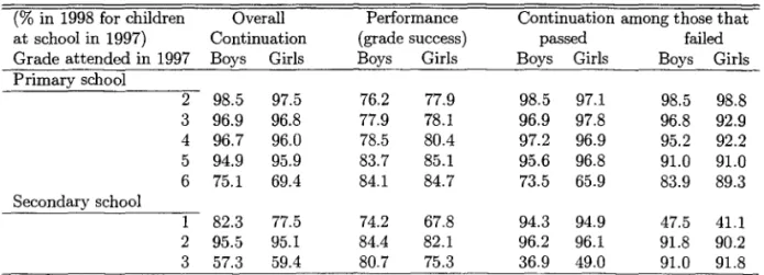
Table 1: Continuation and Performance Statistics4

(% in 1998 for children Overall Performance Continuation among those that

at school in 1997) Continuation (grade success) passed failed

Grade attended in 1997 Boys Girls Boys Girls Boys Girls Boys Girls Primary school

2 98.5 97.5 76.2 77.9 98.5 97.1 98.5 98.8

3 96.9 96.8 77.9 78.1 96.9 97.8 96.8 92.9

4 96.7 96.0 78.5 80.4 97.2 96.9 95.2 92.2

5 94.9 95.9 83.7 85.1 95.6 96.8 91.0 91.0

6 75.1 69.4 84.1 84.7 73.5 65.9 83.9 89.3

Secondary school

1 82.3 77.5 74.2 67.8 94.3 94.9 47.5 41.1

2 95.5 95.1 84.4 82.1 96.2 96.1 91.8 90.2

3 57.3 59.4 80.7 75.3 36.9 49.0 91.0 91.8

Table 1 illustrates the key role of school performance in the decision to continue. There is here again a striking discontinuity at entry into secondary school. The continuation rate at the end of primary school is much lower than the one at any other grade leveI (except after third year of secondary school}. The performance rate is the lowest at the first year of secondary school and there are very high dropping rates after a first year of trying secondary school without success. Table 1 also shows that at the fourth and fifth year of primary school dropping out of school is much more important if the child did not complete his grade. Continuation among those that succeeded is more than 95%. Looking at these statistics, one would like to know if children drop out of school because they failed in their last year of primary school and have to repeat or if this is only due to selection on unobservables. Actually, the policy effect of an educational program and the policy implications can be very different according to what are the causes of school continuation. Is it heterogeneity of students (for example in terms of ability unobserved to the econometrician) that drives dropping out behavior and performance at school or is it only random failure at the end of primary school that causes their drop out? If observed heterogeneity of education paths is due to heterogeneity in unobserved ability or due to unobserved individual random shocks, the policy tools that could effectively improve educational attainment could be very different.

Consequently, there is a clear problem of school continuation in the absence of Progresa, espe-cially at entry into secondary school, and it is intertwined with a problem of performance. Hence, the challenge facing Progresa is to address both issues, i.e., to change the incentives to enroll chil-dren and to improve their performance in school. As we will see in the next section, the design of the program has the potential of effectively addressing both issues.

4Statistics for ali households (eligible and non eligible according to poverty index) in control villages only .

2.2 Incentive Scheme of the Program

The educational component of the program consists in conditional cash transfers to families (given directly to the mother of children) for each eligible child going to school between the third grade of primary school and the third grade of secondary school upon attendance at school. Eligibility for the educational transfers is at the individual leveI for students from poor households in randomly selected treated localities (the poverty status Df the household defines a household levei eligibility criterion for the whole Progresa program). The levei of the grants increases as children progress to higher grades, in order to match the rising income children would contribute to their families if they were working. Additionally, the grants are slightly higher for girls than for boys at secondary school. All monetary benefits are given directly to the female (mother) in the family. Specifically, the rules of the educational program are (Progresa, 2000):

- unconditional annual transfer (almost always in cash) for school materials.

- bimonthly cash transfers depending on gender and grade, conditional on presence at school (at least 85% of school days, i.e., not more than 3 missings a month) from third year of primary school to third year of secondary school. Amounts are reported in Table 2.

- an upper limit for household leveI cash transfers such that if the sum of all individual educational cash transfers and food transfers for a household exceeds some given amount, then educational monthly grants are proportionally adjusted such that total transfers equal the maximum. If a student misses school, the household loses the corresponding proportional receipt.

- students lose eligibility if they repeat a grade twice.

Given these program rules, we can identify several incentive mechanisms potentially affecting the behavior of treated households:

1. All transfers, conditional or unconditional, create an income effect.5

2. The conditionality of educational transfers on school attendance creates both static and dy-namic incentives to enroll. The static incentive is related to the current transfer payment, which reduces the foregone income in going to school. The option of receiving future trans-fers if one stays in school creates the dynamic effect. Rising transtrans-fers with grade leveI further enhance the dynamic incentives.

3. Incentive to perform better at school:

(a) Increasing school attendance may raise students' knowledge and reduce grade repetition.6

(b) Rising transfers with grade give an incentive to perform in school, as repeating the grade Ieads to a Iower transfer than if the student passes to the next grade.

( c) Threat to Iose eligibility if repeats a grade twice.

(d) Negative effect of program termination. In the third year of secondary school, students could prefer to repeat their grade rather than losing the transfer. 7

Table 2: Monthly Progresa Transfers in PesosB Educational Grant by Student 1997 1998 1999 Primary School (Boys and Girls)

1 st and 2rd year O O O

3Td year 60 70 80

4th year 70 80 95

5th year 90 100 125

6th year 120 135 165

Boys in Secondary School

1 st year 175 200 240

2nd year 185 210 250

3rd year 195 220 265

Girls in Secondary School

1 st year 185 210 250

2nd year 205 235 280

3Td year 225 255 305

Further Schooling O O O

Cash Transfer for Food 90 100 125

Household leveI maximum benefit 550 625 750

Denote as T (l, g, 1) the transfer received for gender 9 and completed grade l. T(l,g,l)is

increasing in l until the end of the third year of secondary school after which the program stops: that is program benefits drop to zero very sharply. Note that with the cap on total household transfer and the ruIes on repetition, direct incentives to attend school are a function of family structure and performance in school, giving us variation in the value of transfers across children. In addition, the net incentive depends on idiosyncratic labor market opportunities of children.

6 At the individual levei, more school attendance is expected to improve learning. However, there may be negative

externalities on those students which, in any case, would have attended school regularly if the increased number of children in a classroom lowers the quality of the school. As the data do not indicate the exact attendance in class, we cannot test the presence af these kinds of externalities.

7To get an order af comparison, in Rural Mexico, the average daily wage af a 16-18 years old boys with completed junior high school in the sample was 25 pesos in 1997. A full time work af 20 days per month would generate an income of 500 pesos per month, compared to a maximum of 255 pesos from Progresa transfers. Therefore, heterogeneity of individuais and of labor market expectations and opportunities implies that it is likely that some students will prefer to repeat their third year of secondary school.

BNominal values corresponding to the secand semester af the year (changes occur every semester). Approximately 10 Pesos = 1 US$.

2.3 A Randomized Experiment

The Progresa program operates in ali poor communities (defined by a national marginality index developed from the 1995 census) that have minimal access to primary school and primary care facilities, and all households characterized as poor in these communities are eligible (see Skoufias, Davis, and Behrman, 1999). Poverty status of the household was established at the household leveI prior to the start of the program on the basis of a household census run in October 1997.

Because of the large scale of Progresa, it was decided to implement the program progressively and to design the first years of implementation in order to facilitate evaluation by experimental methods. A subset of 506 of the 50,000 eligible communities was selected to participate in the evaluation. Each of these communities was randomly assigned either to the treatment group where Progresa was implemented starting in 1998, or to the control group where Progresa would be introduced three years later (Behrman and Todd, 1999}. On average, 78% of the population of the selected communities was deemed in poverty and hence eligible for the programo All households (eligible and non-eligible) of both types of communities were then surveyed twice a year during the three years of the evaluation. These experimental communities are located in seven states (Guerrero, Hidalgo, Michoacan, Puebla, Queretaro, San Luis Potosi, and Veracruz). There are 320 treatment localities and 186 control localities in the experimento Program benefits began in May 1998. The unbalanced sample, including all individuaIs present at some point in time between October 1997 and November 1999, is of 152,000 individuaIs from 26,000 households. Because transfers are generous, almost ali eligible families chose to participate (97%).

Two factors make the study design especially rigorous. One is the random assignment of commu-nities into treatment and controIs. The other is the paneI dimension of data collected on househoIds and their members before intervention of the program and subsequently every 6 months throughout the two-year experimental period. We use data from the first two years of evaluation, which include a baseline survey in October 1997 and the follow up surveys in October 1998 and November 1999. We thus have information on enroliment during three consecutive school years 1997-98, 1998-99, and 1999-2000, and on performance in school during academic years 1997-98 and 1998-99.

A first look at statistics contrasting control and Progresa communities in Table 3 show that enroll-ment and passing rates are higher in the Progresa than in the control communities, although this effect is small when all grades are combined.

Overall Performance Continuation among those that

Grade attended Continuation (grade success) passed failed

in 1997 ControI Treatment Control Treatment ControI Treatment Control Treatment

Primary school

2 98.0 98.6 77.1 77.6 97.8 98.8 98.6 98.1

3 96.8 98.1 78.1 83.1 97.4 98.3 94.9 97.3

4 96.4 97.6 79.4 82.7 97.1 98.1 93.9 95.3

5 95.4 97.3 84.4 85.9 96.3 97.8 91.0 95.0

6 72.4 79.9 84.4 85.8 69.8 78.1 86.5 91.2

Secondary school

1 80.1 87.3 71.2 75.2 94.6 96.5 44.2 59.7

2 95.3 94.9 83.3 85.3 96.2 96.1 91.0 87.7

3 53.0 56.4 78.2 78.9 42.4 49.0 91.4 83.9

The population of interest is that of poor people who are designated as eligible for Progresa. Those in the treatment group can receive the Progresa benefits and those in the control group cannot. The average household size is around 7 people. A little less than one third of individuaIs in the sample are indigenous. 15% of household heads have an educational leveI less than primary school, 30% completed primary school, and 52% completed secondary school.

3

A Dynamic Educational Model with Schooling, Effort, and

Per-formance

In order to study the effect of the program on education, we elaborate a dynamic schooling model able to show that it may affect both enrollment and learning behavior. The modelling of schooling decisions is generally done by assuming that the household decision maker maximizes the net expected income of a child. In this calculus, earnings are increasing with education, but education has a cost charged against this income which includes the opportunity cost of the time spent studying instead of working. As we have seen in the descriptive statistics, failure to pass a grade is a serious problem in Mexico's poor rural communities. To face up to this problem, Progresa was purposefully designed to be conditional not only on grade leveI but also on school performance. Moreover, the role of class repetition in the decision to drop out of school can be very important and the analysis of schooling decisions can be very misleading if one does not account for this phenomenon.

conditional on a set of exogenous characteristics that could affect the wage or costs of schooling. All these characteristics are removed from the theory to simplify notations but do appear in the econometric specifications.

Assume that the decision maker is the household beneficiary, in this case the mother, and that she maximizes the discounted lifetime expected utility of the child. For a child, Iet l be the grade completed at the beginníng of an academic year and g hís gender. A chiId who has completed grade l is assumed to be automatically accepted in grade l

+

1 if he enrolls at school. Then, according to Progresa ruIes, if the household is eligible, the household beneficiary (generally the mother) is entitIed to an educational transfer of T (l,g,p). For poor people, p = 1 in randomly seIected treatment villages and p = O otherwise (with T (l, g, O)

==

O). Let s be a variabIe equal to one if

the child is actually going to school and zero otherwise. Let 7r, the educational performance of the chíld, be a function of his schoollevell, and an individual Iearning effort choice e: 7r (l,

e).

This effort variable is meant to represent individual actions of the student such as attention in classes, being late at school, and studying at home. As educational learning and skills are not perfectly observable by the teacher, we assume that the student wíll complete grade l

+

1 if and only if s

=

1 and 7r Cl, e) ~ é, where ê is a random variable with c.d.f. F and p.d.f.

f.

7r depends on l because

the leveI of performance required to pass varies with grade leveI. This function will depend on the selectivity of the educational system settled by the government. We will later consider two cases: one where e is exogenous, and the other where e is endogenous. The function 7r can also depend on characteristics x of the student (a vector including individual and other characteristics like for example distance to school) but we don't need to explicitly introduce them in the theoretical model as long as they are exogenous.

Grade progression is determined by the following rule:

lt

+

1 if St = 1 and 7r Clt, et) ~ êt (1)

with the following assumptions:

Assumption 1 The probability of success P(lt+l = lt

+

Ilet, St = 1) = F o 7r (lt, et) is increasing and concave in effort et.

This assumption is satisfied when the performance function 7r (1, e) is increasing and concave in

..

Assumption 2 The earnings function w (g, l) is increasing in the acquired leveI of education l.

All these variables refer to year

t

when the index

t

is used. We assume that the cost for a child for going to school in year t, denoted c (et) depends on the learning effort et (plus the cost of transportation, and other costs of enrollment).

Assumption 3 The cost function

c( e)

is increasing and convex in

e,

the leve} of learning effort at school.

Then, sending a child to school in year t costs c (et) -r(lt, g,p), while not sending him generates earnings w(g, lt), the opportunity cost of enrolling the child in school. Assuming that the decision process in the household results in the maximization of the intertemporal expected benefits for the child w(lt, g, p, St), the value of enrolling a child at the beginning of year t (St = 1) or that of not enrolling him (St

= O)

knowing his completed grade lt, his gender g and eligibility p can be written recursively as follows:

w(lt,g,p,l)

w(lt,g,p,O)

max{ r (lt, g,p) - c (et)

+

,BE[ max w(lHl, g,p, St+Ü I St

=

In

et 8t+1 E{O,l}

W (g, lt)

+

,BE[ max W(ltH, g,p, St+l)

I

St

=

O]

st+1E{O,l}

with ,B the discount factor and ltH following the law (1).

(2)

(3)

Because of the uncertainty of grade progression, parents revise their expected optimal choice at the beginning of each schooling year.

The value function for a child of education lt, gender g, and eligibility p can be written:

cp(lt,g,p) = max w(lt, g,p, St)

StE{O,l} Substituting in expressions (2) and (3) gives

w(lt,g,p,l)

w(lt,g,p, O)

max{ r (lt, g,p) - c (et)

+

,BE[cp (lHl, g,p)

I

St =

In

et

w (g, lt)

+

,BE [cp (lHl, g,p) I St

=

OI

=

w (g, lt)

+

,Bcp (lt, g,p)

because P(ltH = lt

+

1

I

St = O)

= O.

This implies

(4)

cp (lt, g, p)

=

max{ T (lt, g,p)

+

max{,BE[ cp (lHl, g, p)

I

St

=

1] - c (et)}, w(g, lt}

+

,Bcp(lt, g, p)} (5) et

Then, we can show the following proposition:

Proof. See Appendix Gl. •

IntuitiveIy, we expect the value function cjJ to be increasing with completed grade. Though one could imagine that at the end of secondary school, when transfers stop, the vaIue function could drop, this is something our empirical observation in Mexico does not support. Being more educated is aIways vaIuabIe and the Progresa transfers, whatever their positive or nega tive effects on enrollment and Iearning efforts, did not change the monotonicity of the value of education. In the sequeI of this paper, we will suppose the following.

Assumption 4 The value function cjJ is always increasing with completed grade.

In Appendix B, we show which sufficient conditions on the primitives of the model ensure that the endogenous value function cjJ is always increasing with completed grade. However, rather than assuming these "reasonable" sufficient conditions we will simply assume that cjJ (l, g, p) is increasing in l.

3.1 Program Impact on Efforl and Performance

The theoretical impact of the conditional transfer program on the school performance of children will depend crucially on the assumption of whether students can adjust their Iearning effort or noto We could consider, as often done, that learning activity depends on the exogenous characteristics of children and cannot be adjusted once presence at school is required. On the contrary, some consider that higher returns to education (in a very broad sense) constitute an incentive for students to study and learn more. Introducing an endogenous learning effort, the maximization of the value function implies that learning effort is chosen conditional on enrollment so as to maximize

T(lt,g,p) - c(e)

+

(3E[cjJ(lt+1,g,p)

I

s

=

1].

Proposition 2 VVhen the learning effort e is a choice variable, it is zero if cjJ(l

+

1, g,p) ::; cjJ(l, g,p) and strictly positive if cjJ(l

+

1,g,p)

>

cjJ(l,g,p). In this latter case, learning effort can be either

increasing or decreasing with grade. The expected performance at school can also be either increasing

or decreasing with grade.

Proof. See Appendix C.2. •

When the optimallevel of effort is positive, it is given by the first order condition:

(3[cjJ(l

+

1, g, p) - cjJ(l, g,p)]f o n(l, e*)

~:

(l, e*) = c'(e*)

(6)

,

CorolIary 3 Ifcp(l+l,g,p)-cp(l,g,p)

(>0)

decreases inl and ~7

>

O thene* and P(lt+l = lt+ll St = 1) decreases in l i. e. when the value of education is an increasing concave function and the educational system is less and less selective for higher grades, the learning effort is decreasing and

the probability of failure increasing with l.

If cp(l+ 1, g, p) -cp(l, g,p)

(>0)

increases in l and ~7

<

O then e* and P(lt+l

= lt

+

1

I

St

= 1) increase

in l i. e. when the value of education is an increasing convex function and the educational system is more and more selective for higher grades, the learning effort is increasing and the probability of

failure decreasing with l.

These results call for taking into account heterogeneity of treatment effects since the theoretical impact of the program on performance depends on the sign of the difference ~ [cp(lt

+

1, g, p)

-cp(lt,g,p)] according to the following proposition. For notational ease we use ~ as the operator for

differencing functions

H(p)

as follows ~H(p) =

H(I) - H(O).

Proposition 4 When the learning effort is fixed exogenously, the performance at school or

proba-bility to pass a given grade do not depend on treatment

(&,;;

=

O and

~P(lHl

= lt+11 St

=

1)

=

O).

When the learning effort is a choice variable, treatment raises effort and performance at school in terms of probability to succeed in a given grade if cp(lt

+

1, g, 1) - cp(lt, g, 1)

>

cp(lt

+

1, g, O) - cp(lt, g, O)

and reduces effort and expected performance if cp(lt

+

1, g, 1) - cp(lt, g, 1)

<

cp(lt

+

1, g, O) - cp(lt, g, O).

It is constant if cp(lt

+

1, g, 1) - cp(lt, g, 1)

=

cp(lt

+

1, g, O) - cp(lt, g, O).

Proof. If the learning effort is fixed exogenously, then ~P (lHl

= lt

+

1

I

St

=

1)

=

O i.e. the eligibility has no effect on the probability to successfully complete the grade leveI on children going to school. If the effort is chosen endogenously, then et depends on p. As shown previously, if

cp (lt

+

1, g,p) - cp (lt, g,p) :::; O, then e;

=

O. If cp (lt

+

l,g,p) - cp (lt, g,p)

>

O, then e; satisfies (6). With assumptions 1 and 3, the implicit function theorem implies that e; is increasing in p if

cp (lt

+

1, g, 1) - cp (lt, g, 1) 2 cp (lt

+

1,g, O) - cp (lt, g, O) and decreasing in p otherwise. 7r (l, e) is an increasing function of e so the same applies for performance. _

,

The previous proposition gives us an empirical test of whether the learning effort is endogenous or exogenous which is of great importance for education policies. In the following corollary, we give the explicit identifying assumption required:

Corollary 5 Under random treatment and the unconfoundness assumption that treatment does not

affect the performance and evaluation technologies 1T and F (p Jl F o 1T is sufficient):

lf treatment affects the probability to pass a given grade then the learning effort is endogenous.

lf treatment does not affect the probability to pass a given grade then the learning effort is exogenous.

Hence, with the randomized experiment implemented by Progresa, we can test if the learning effort of students is indeed a choice variable affected by the transfer incentives.

3.2 Program Impact on the Enrollment Decision

The decision of enrollment is derived from the comparison of the value of going to school and not going. Define the decision to enroll the child at school by St = l{v(lt,g,p);?:O} (1 for school enrollment and O otherwise) where v(lt, g,p)

=

w(lt, g,p, 1) - w(lt, g,p, O) is the difference between the two conditional value functions.

The following proposition is straightforward and shows the derivatives of v(lt,g,p) with respect to the program treatment p which represents the effect of treatment on the propensity to choose schooling over working (with a slight abuse of notation because [)v(~~g,p) = v(lt,g, 1) - v(lt,g,O)).

Proposition 6 The program impact on the value of going to school compared to not going is:

ôv(lt,g,p)

=

( l I ) ôp T t,g,

ô

+

jJ{ [cp(lt+1,g,1)-cp(lt,g,1)] ôpP(lt+1=lt+1/St=1)

ô

+ P(lt+1

=

lt

+

1 / St

=

1) ôp[cp(lt

+

1,g,p) - cp(lt,g,p)] }

Proposition 6 shows that [)v(~:,p) is composed of several terms:

The first term, T( lt, g, 1) ~ O, is the direct incentives to go to school provided by the educational transfer to be received by eligible students going to school.

The second term is the discounted expected marginal value of program eligibility composed of: - The marginal increase of the probability of succeeding in grade progression times the marginal value of getting an additional year of education:

[<p(lt

+

1, g,p) -cp(lt, g,p)] ~P(lt+1

=

lt+ 1 / St = 1). It comes from the fact that higher incentives to succeed are given to eligible students. This term is zero if the learning effort is exogenous. If the con-ditions for Proposition 10 are valid in the case of Progresa, we have that cp(lt+1, g,p) -<p(lt, g,p) ~ O.

- The increase provided by treatment of the marginal value in getting one additional year of ed-ucation, given the probability of successfully completing the current grade, P(lt+l = lt

+

1

I

St = l)g,[4>(lt

+

1,g,p) - 4>(lt,g,p)].

Moreover, according to proposition 4, gpP (ltH

=

lt

+

11 St

=

1) and gp[4>(lt

+

l,g,p) - 4>(lt,g,p)]

are of the same signo This model clearly shows the implications of the program on the value for children of going to school compared to that of not going. In particular, it helps explain that the incentives provided by eligibility do not only depend on the reduction of the opportunity cost of schooling by the conditional transfers but also on the additional value provided by the expecta-tion to receive transfers the year after and the expected value of being more educated. Therefore, the program impact has no reason to be simply proportional to transfers received. According to this model, the treatment effect of the program should be heterogeneous across individuaIs with different grades, gender but also across all characteristics affecting future wages for example.

Another implication is that the incentives to go to school represented by 8v(~:,p) depend on the cash transfer corresponding to the current grade, the conditional cash transfers for upper grades but not that of lower grades, and on the probability of grade progression.

As the value functions depend on the design of the program, effort will depend on the pattern of potential future transfers corresponding to higher grades. When effort is fixed, we could show unambiguously that the program impact ought to be larger on the first year of implementation than on the second year because the end of the program is closer as time is running (even without any arguments relying on econometric estimation issues like selection on unobserved heterogeneity that we will address later). The impact of the program depends naturally on the year being evaluated. In the case of Progresa, the program being a fixed 3 year term, its impact in the first year will be different from that of the second year since the remaining years of transfers are different even if the transfer schedule by grades and gender is constant.

Note also that even if the transfer function for some grade L and gender 9 is zero, T(l, g, 1) =

T(l,g,O) = 0, we still have 8v(~,p) =I-

°

if for some grade L'

>

L, T((l',g,l)

>

O. Because of the expected benefit from transfers in higher grades, the cash transfer program also generates incentives in favor of schooling even if the student is not entitled to receive any grant in his current grade. In the particular case of Progresa, this indicates a possible incentive to schooling even in the first and second year of primary school for eligible students although they receive nothing in their current grade.

4

Identification and Econometric Evaluation

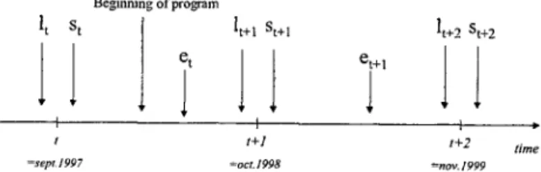
The theoretical model developed in the previous sections gives testable implications regarding the impact of the government sponsored cash transfer program on enrollment decisions and performance outcomes. We exploit this by estimating transition probabilities from grade to grade P(lt+1 = lt+1J St = 1) and enrollment decisions9• Figure 1 shows the time line of events and decisions. We can specify the structural econometric model by choosing parametric assumptions on functional forms and random terms and derive the corresponding reduced formo

Timing of School ResuIts and Enrollment Decisions

Beginning of program

It St

j

It+l St+l It+2 St+2

1 1

et

1

1

et+1

1

1

1

1

1+1 1+2 _time

=sept./997 =oct./998 =noy./999

It : approved grade at beginning ofperiod [t,t+ I] observed

just before t

St : enrollment decision for period [t,t+ I] takenjust after t

knowing It

Figure 1: Timing of the Dynamic Decision Process

4.1 Econometric Specification

Adding exogenous characteristics Xt to the grade progression model (1): P (lHl = lt

+

1 J St

=

1)

=

F o 7r (Xt, lt, et) where e; is endogenously determined and depends on Xt, lt, g, p. Therefore, we assume that the discrete grade progression follows:

(7)

where "Ilt,g' Bz"g are vectors of parameters specific to grade and gender, Xt is a vector of exogenous variables (including Xt, lt,

g),

and r.p is a c.d.f. (for example logistic or normal)10.

Assuming that some unobserved component

ç

of cost c

(eHd

or wage w(Xt+1' g,

lHd

is randomly

9Most estimation will be based on parametric maximum likelihood. Actually, as the observed outcome variables are binary, a fully non-parametric identification of this binary choice model is impossible. However, the semiparametric identification of binary choice models is possible with some assumptions like location and scale normalization (Manski, 1985, 1988) but given the number of explanatory variables used in our regressions we will use simple parametric estimation methods.

1 °This specification is consistent with the theoretical model for example (but not only) if the c.d.f. F of ê is normal

distributed with logistic or normal c.dJ. cp, we can get a semi-structural model of the probability of continuing school (see section 6). We first focus on the reduced form of the model, which does not allow to decompose the effect of the program on each incentive component identified in the theoretical model. However, it does allow to evaluate the total program impact an enrollment and performance at school and is more robust to mispecification than the semi-structural model. By linearization of the grade progression probability, we establish the following reduced form

where Zt+l is a vector of exogenous variables (left implicit in the set of conditioning variables for notational ease). Of course, since the design of the program is such that transfers are gender and grade specific, coefficients a' s will be allowed to be gender and grade specific (implicitly allowing the effect of future transfers expectations to affect this probability). Our model thus leads us to estimate the impact of the program on two equations of interest: the probability of continuing school P(St+1

=

1

I

St

=

1) and the prabability of progressing in grade P(lt+! =

lt

+

1

I

St = 1).

4.2 Identification of the Program Impact and the Dynamic Selection Problem

As shown by Cameron and Heckman (1998), the estimation of school transition mo deIs faces a problem of dynamic selection bias. Even if unobserved factors entering the schaol transition model are distributed independently of observable characteristics in the population enrolling in the first year of primary school (for example), the distribution of unobserved characteristics of students in the secand year af primary school will be truncated and not independent af the distribution of observable characteristics because of the educational selectian of students. This dynamic selection of the population of students introduces a bias in the estimation of transition models. Here, we would certainly meet this difficulty in the estimation af probabilities to enroll at school and probabilities to successfully pass a grade. However, we are interested in the impact of the program on these transition prababilities. With randomization of treatment, the evaluation of the average program impact will not be biased by this dynamic selection problem. We explicitly farmulate the necessary assumptions for identification in order to establish the relationship between randomization and the dynamic selection problem.

Transition probabilities conditional on the vector of observables Wt+1 = (Zt+1, Xt, lt+1,

sd,

the treatment dummy p E

{O,

I} and unobserved characteristics (j can be writtenl l

(9)

..

.

-where 'Ij; (o) a real valued function.12 It is to be noted that with these notations, t'lj;(wt+l,p,8) can be seen as corresponding to the marginal treatment effect defined by Heckman and Vytlacil (1999, 2000a, 2000b, 2002) since the unobserved variable

e

is likely to affect participation of an individual into the corresponding grade where treatment (Progresa program) is receivedo

As

8

is unobserved, we cannot identify E(St+l

I

Wt+l,p,8) but rather the average E(St+1

I

Wt+l,P) =

Eõ[E(St+1

I

wt+l,p,8)]0 The parameters of interest that we would like to identify are the average program impact

(10)

and the average effect of some covariates Wt+1

{)

-E7J[-!:)-E(St+l

I

Wt+l,p,e)]

UWt+l

(11)

Cameron and Heckman (1998) showed clearly that even if the distribution of

8

is independent of

Wo

(8

l i wo), this random effect assumption for the initial schooling stage will not be true for the subsequent ones because of the selection of students; that is, in general e

..JX'

Wt+lo This dynamic selection bias implies that

The value

~E

_VWt+l (St+l

I

Wt+l,p) is thus a biased estimator of

&()[~'Ij;(Wt+l,P,

_UWt+l

8)]

(the deriv-ative of the average E7J7fJ(Wt+1,p,8) is not equal to the average derivative)o In the schooling transition probabilities, we will have biases equal to B(Wt+l, 1) = 8w~+l [E7JE(St+l

I

Wt+l,

1,8)]

-E7J[8w~+l

E(St+1

I wt+l,

1,8)]

for the treatment population and to B(wt+l, O)

=

aW~+l

[E7JE(St+l

I

Wt+l,O,8)J -

~[8w~+l

E(St+l

I

Wt+1,

0,8)]

for the controI populationo Each bias being difficult to sign and quantify a priori (as in Cameron and Heckman, 1998), the only solution is then to model the unobserved component

8,

for exampIe by using the Heckman and Singer (1984) technique in-troducing a discrete non-parametric distribution for

80

However, this is still subject to an arbitrary choice in the modelling of

8

which could be multidimensional.

However, as proposition 7 shows beIow, we do not encounter the same problem when evaluating the average program impact

{)

op E(St+l

I

Wt+1,p)

=

E(St+l

I

Wt+l,P

=

1) -

E(St+l

I

Wt+l,P

=

O)

Actually, first note that randomization implies that treatment is orthogonaI to observed and unob-served characteristics

(12)

..

~~~~~~--~~~---which implies that

P lL

o

I Wt+l·

Proposition 7 lf treatment P E {D, I} is orthogonal to the distribution of unobserved

characteris-tics conditional on observables Wt+l that is

P lL O

I

Wt+l (13)

then

(14)

Proof. Proof in Appendix C.3. •

With the randomization of treatment, property (13} is satisfied and Proposition 7 applies. Recall that aW~+1 E(st+l I Wt+l,p) is not identifiabIe because of the dynamic seIection problem. However, we might still be interested in identifying the change in the effect of Wt+l on the tran-sition probability due to the program P or how the program impact depends on Wt+l which is

gpaW~+1

E(St+l

I

Wt+l,p) =

aW~+1

E(St+l

I

Wt+l, 1) -

aW~+1

E(st+l

I

Wt+l, O). The question is then to compare B(Wt+l, 1) and B(Wt+l, O) because if both biases are the same in the treatment and control groups then aa aw_{p t+1} a E(st+l

I

Wt+l,p)

=

aap&()[-a _Wt+1 a V;(Wt+l,P,

ê)]

would allow to identify the dependence of the average program impact on Wt+l. We have the following Proposition:

Proposition 8 The average treatment effect ~[g a ~ V;(Wt+l'p,O)] is identified and equal to

p Wt+1

g

a

~ E (St+l

I

Wt+l,p) if one of the following condition is satisfied13 p W t+1

ar

J

- 8

-

J

8

-E(st+l

I

Wt+l, 1, B ) - 8 k d>"(B

I

Wt+l) = E(st+l

I

Wt+l, O, B ) - 8 k d>"((}

I

wt+ú

wt

+

1 wt

+

1

(16)

Proof. See Appendix C.4. •

Condition (15) means that the distribution of O does not depend on wf+l i.e. that there is no dynamic seIection bias in the direction of

wf+l'

Condition (16) means that the marginal treatment effect lE(st+l

I

Wt+l'p,O) averages to zero when integrating with respect to a

~

d>"(O

I

Wt+l)

Ui' W_t+₁

which is always the case if aa E(st+l

I

Wt+l,P, O) is constant across O because

J

a ~ d>"(O

I

Wt+l) = O

p W_t+1

since

J

d>"(O

I

Wt+l)

==

1. Therefore, this is always true if the average treatment effect

~E(st+l

I

Wt+l,P, O) does not depend on Wt+l.

13T he notation À is used to designate cumulative distribution functions. For example À(Õ

I

Wt+d is the c.dJ. of Õ

conditional on Wt+1.

..

In the present case, neither assumption (15) nor (16) has to be valid given the randomization procedure. (15) will be wrong as soon as there is some dynamic selection which is now a widely accepted feature in education transition models and (16) is unlikely to happen as soon as the treatment effect gpE(St+l

I

WHl,p,O) depends on covariates Wt+l. Therefore, the randomization process insures only the identification of the average impact ~E(St+l

I

WHl,p).

The same argument can be applied to the performance probability

P

(IHl = It

+

11 St = 1). The randomization condition (13) is sufficient to ensure that the dynamic selection bias present in the estimation of the conditional probabilities P (SHl = 1

I

St = 1) and P (IHl = It

+

11 St = 1) will be the same for treated and untreated sample and will then cancel out in the estimation of the program impacto

Condition (12) requires that the joint distribution of observables and unobservables be independent of treatment i.e. be the same across treated and control samples. This condition cannot be tested but an implication of it on the marginal distribution of observables can be checked and is empirically validated for data in 1997 by Behrman and Todd (1999). However, we can assume safely that the randomization of the program placement in the case of Progresa is such that the condition (12) is true at the beginning of the program in 1997. Randomization provides an instrument which is orthogonal to all other variables and in particular to unobserved random variables affecting the conditional probabilities. However, in 1998, the program impact being probably non zero (as the empirical results will confirm) we can expect that this will not be true anymore and the dynamic selection bias wiU not cancel out across treatment and control groups. Therefore, we expect that the conditional probabilities estimates of the program impact between 1998 and 1999 wiIl be biased by a dynamic selection bias due to the dynamic impact of the programo Intuitively, we for example expect that the program having a positive effect on the propensity of continuing schooling, it will select individuaIs with (on average) lower unobserved factor also causing an increase in the individual propensity to go to school (like unobserved ability). This in turn would bias downward the probability to succeed in class and to continue the following year. Then one possible solution is to use the Heckman and Singer (1984) technique to estimate these conditional probabilities with discrete non parametric unobserved heterogeneity that one has to estimate jointly to the parameters of the mode!.

4.3 Identifying the Elasticity of the Program Impact to Cash Transfers

Until now we have investigated the estimation of the average program impacto However, one may be interested in the elasticity of the program impact to the amount of cash transfers defined by

where T is the transfer received by the student (the previously defined treatment dummy is p = l(T>o))·

To expIain the identification method, we show the following proposition:

Proposition 9 Assume that there exísts a random varíable w~+l such that the transfer ís T

r

(g, l, p, W~+ 1) and the followíng assumptíons are satísfied:

The average treatment effect trE(St+l

I

Wt+l, T) does not depend on w~+l i.e.

a a

- a ' (aTE(St+l1 Wt+l, T)) =

o

wt

+

1

The program rule reg, l, p, w~+l) ís such that

(Exclusion Restriction)

(Known Conditionality of Program Rule on ObservabIes)

and does not depend on unobservables

e

(Program Rule Independent of Unobservables}

The observed component w~+l ís independent of unobserved factors

e

condítíonally on Wt+l

(IV assumption)

Then trE(st+l

I

wt+l,T) is ídentified14 with

~[trE(St+l

I

wt+l,T,ê)J.

Proof. Proof in Appendix C.5 . •

In the Progresa program, this identification is provided by the maximum rule as follows15 . The Progresa ruIes stipulate that household transfers cannot exceed some given maximum amount of money and impose a proportional adjustment rule for individual benefits. Table 4 gives exampIes of this proportional adjustment in terms af transfers to be received. The last column shows what is the transfer due for each child given this adjustment for family A and B which otherwise would get more than the maximum amount allowed while family C does not reach this amount. This monthly amount corresponds to what is lost if a chiId misses school without justification.

Table 4: Example of the Maximum Rule

140f course only within the range of variation of T in the data observed.

15Without this rule, the value Df transfers T = 7(g,l,p) are conditional only on gender 9 and grade I which are observable characteristics very likely to be correlated with the individual unobservable components g (because Df the dynamic selection problem). Then, if transfers do not vary across individuaIs (conditionally on Wt+l), ;TE(St+l

I

Example of the Maximum Rule in 1997 Progresa Grant

Without With Proportional

Family A:

One Boy in Secondary School (1 st year) One Girl in Secondary School (2nd year) One Girl in Secondary School (3Td year) Total received by household

Family B:

One Girl in Secondary School (1st year) One Girl in Secondary School (2nd year) One Boy in Secondary School (3Td year) Total received by household

Family C:

One Girl in Primary School (6th year) One Girl in Secondary School (2nd year) One Boy in Secondary School (3Td year) Total received by household

Adjustment

175

205

225

605

185

205

195

585

120

205

195

520

Adjustment

175

x 550

=

159

~8g

x 550

=

186

!~!

x 550

=

205

550

185

x550

₌

₁₇₃

~ag

x550

₌

₁₉₃

~~g

x550

₌

₁₈₄

585

550

120

205

195

520

Noting T' = T(g, l,p) the total transfer that the household would receive for a child in absence of this maximum rule and Mt+l the maximum amount of money the household can receive at time

t

+

1, the actual transfer received is the known function

. {Mt+l }

T=T(g,l,p)mm -rr,1

The assumption needed for identification is that the random variable min { M

T

;! ,

1 } does not affect

the average treatment effect a~E(St+l

I

Wt+l, T) i.e. that given observables Wt+l the average effect of transfer T on schooling St+l is constant across values of T'. Cancretely, it means that the effect of transfer T on individual schooling can depend on observable characteristics of a student but that conditionally on these characteristics Wt+l there are other observable characteristics that affects

T' but not the treatment effect. For example, the number of children of the household which generates variation the individual transfer amount (because some reach the maximum and others not) may have a direct effect on the average treatment effect. However, conditionally on the number of children with for example equal number of boys and girls, it may be more reasonable to assume that the order of gender of children does not affect the average treatment effect directly while it provides some variation in the amount of transfers received. Table 4 shows examples of families with the same number of children, the same number of boys and girls but for which individual transfers of the girl in the second year of secondary school vary because of this rule of the maximum. The presence at school of a second year secondary school girl will not bring the same transfer if she belongs to family A, B or C in the example of Table 4.

We therefore exploit this kind of variation and assume that conditionally of wt+l (which in-clude the number of children) the fact that the household reaches the maximum of not is randam

and uncorrelated with the unobserved characteristics

7i

because it comes mainIy from the random distribution of genders within the children. The conditions of identification given by Proposition 9 are then pIausibIe even if not testabIe.

5

Empirical

ResuIts

and Policy Implications

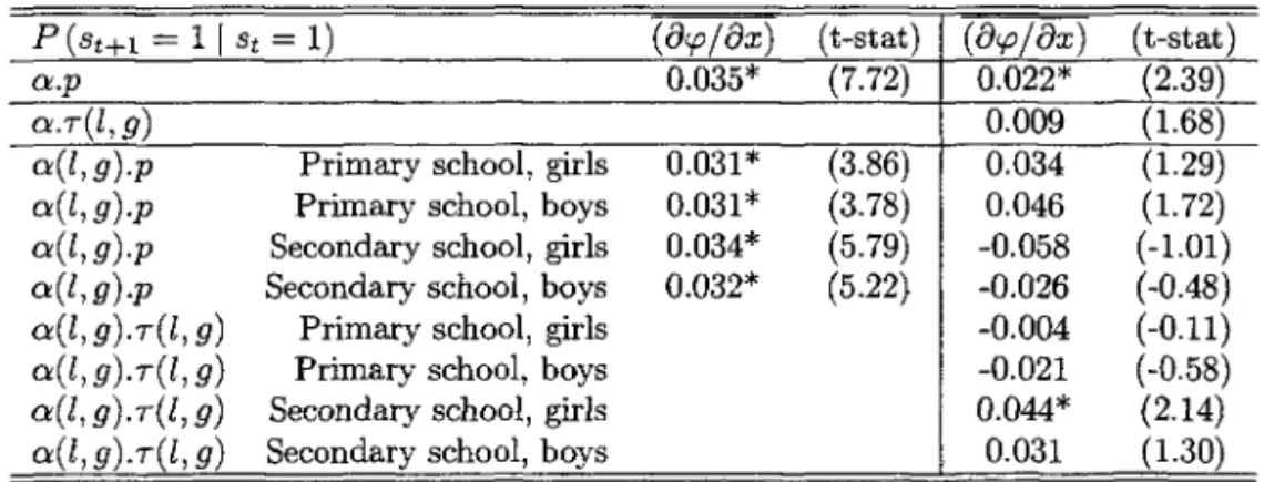
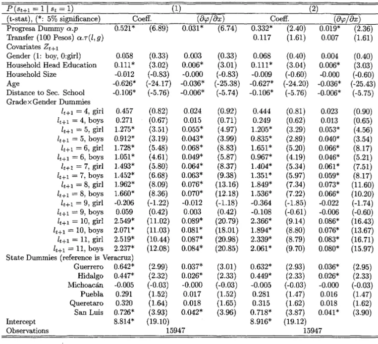
Given the identification issues shown in section 4, we first compute the average treatment effects on transition probabilities of the reduced form model i.e. the probabiIity of continuing school

P(St+l = 1

I

St = 1) and the probability of progressing by one grade P(lt+l = lt

+

1

I

St = 1) by estimating a Iogit of the outcome discrete variable conditional on treatment and households characteristics. In this case, the average effect is the coefficient of the dummy variable for treatment

(p). In a second step, using the Progresa ruIes according to the identifying strategy described in

section 4.3, we identify the effect of the transfer value on these outcome variables. In the data, the sample proportions of deviations from the pre-set amount because of the maximum benefit ruIe is of 14% in 97, 9% in 98, and 13% in 99.

In the following, the completed grades are numbered as follows:

Table 5: Grades targeted by the program

Completed grade Value of Progresa program Grade attended

I active if enrolled if enrolled

Primary school pt year 4 no 2nd year of primary

2nd _{year 5 yes 3}rd _{year of primary}

5th _{year 8 yes 6}th _{year of primary}

6th _{year 9 yes 1 st year of secondary}

Secondary school 1st _{year 10 yes 2}nd _{year of secondary}

2nd _{year 11 yes 3}rd _{year of secondary}

3rd _{year 12 no other}

Recall that the Progresa program, beginning at the third year of primary school and ending at the third year of secondary school, is active for individuaIs going to school with completed grades between 5 and 11.

5.1

Performance

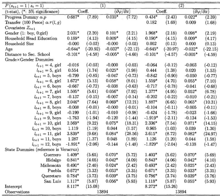
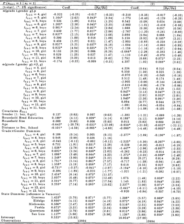
ResuIts of the estimated probability of grade progression during school year 1997-98, are fully reported in Tables P98-1, P98-2 and P98-3 of Appendix DHi• These probabilities are estimated using a Iogit modeI17 _{with standard errors robust to heteroscedasticity and the means of marginal effects}

16Table P98-1 shows the estimates Df the average treatment effects over ali grades. Table P98-2 shows the average program impact by gender for primary and secondary school. Table P98-3 shows the average program impact by grade and gender. Moreover, ali these Tables also present the estimates ofthe elasticity ofprogram impact to transfers (17) which is identified according to Proposition 9.

17Results using a probit model are very similar. Though coefficients are different in absolute value as usual, means of marginal effects are very elose when estimating with logit or probit.

are presented together with coefficient estimates. Means of marginal effects are noted

(or.p/ox)

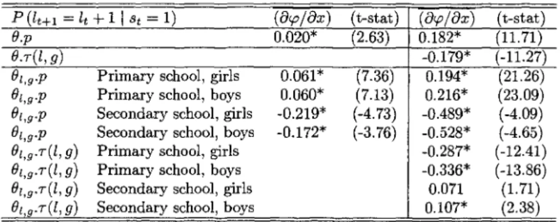
and computed as means of the observation by observation marginal effects,of each variable. Tables P98-1, P98-2 and P98-3 also present the full set of dummy variables inc1uded in the regressions and shows in particular that household size has a negative effect on performance, household head education and gender have no significant effect, and the student's age a negative one. In summary tables 6, 7, 8, and 9, the first two columns present the results of estimating the average impact of transfers and the last two columns present the results when estimating the elasticity to transfers.

According to Proposition 7, the average program impact (equation (14» is identified with the random experiment implemented. Table 6 presents the most important estimates. First, the average program impact on students is significantly positive. The average treatment effects present a 2 percentage point increase in the probability to successfully complete the grade. The average elasticity to transfers of performance (rows denoted by 8.7(l,

g»

is negative but Table P98-3 shows that when the program impact is estimated by grade and gender, there is no more negative elasticity18. The average treatment effect by gender for primary and secondary school are very different. The means of marginal effects for primary school are positive with a 6.1% increase in performance both for boys and girls while it is negative at secondary school with means of marginal effects of -21% for girls and -17% for boys. This result can be interpreted by the fact that the cash transfer program has a negative impact on learning effort because students want to remain as long as possible in the programo At primary school, they seem to increase their learning effort (willingness to benefit from higher transfers, better learning condition thanks to the program benefits in cash but also including better health care and nutrition components) but at secondary school the program has a negative effect because the probability of repetition increases.

Concerning elasticity to transfers, they are still negative at primary school but positive at secondary school with means of marginal effects for girls of 7% and 10% for boys meaning that a 100 pesos increase in transfers of secondary school would increase the performance probability of 10% for boys and 7% for girls (in all Tables, the value of transfers are in hundreds of pesos). Finally, Table P98-3 in Appendix D also shows the average treatment effect by gender and each grade leveI of primary and secondary school. It appears that a significant positive effect is found for the third year of primary school with means of marginal effects of 5.2% for girls and 4.3% for boys. Moreover, a negative significant effect is found on the first and third year of secondary school with means of marginal effects of 37% for girls and 29% for boys in the first year and 19% for girls