A high-resolution mass spectrometer to measure atmospheric ion composition

(1)

AMTD

3, 599–636, 2010

A high-resolution mass spectrometer to measure atmospheric

ion composition

H. Junninen et al.

Title Page Abstract Introduction Conclusions References Tables Figures

◭ ◮

Back Close Full Screen / Esc

Printer-friendly Version Interactive Discussion

Atmos. Meas. Tech. Discuss., 3, 599–636, 2010 www.atmos-meas-tech-discuss.net/3/599/2010/ © Author(s) 2010. This work is distributed under the Creative Commons Attribution 3.0 License.

Atmospheric Measurement Techniques Discussions

This discussion paper is/has been under review for the journal Atmospheric Measure-ment Techniques (AMT). Please refer to the corresponding final paper in AMT

if available.

A high-resolution mass spectrometer to

measure atmospheric ion composition

H. Junninen1, M. Ehn1, T. Pet äj ä1, L. Luosuj ärvi2, T. Kotiaho2,3, R. Kostiainen3, U. Rohner4, M. Gonin4, K. Fuhrer4, M. Kulmala1, and D. R. Worsnop1,5

1

Department of Physics, P.O. Box 64, 00014, University of Helsinki, Helsinki, Finland 2

Department of Chemistry, P.O. Box 55, 00014, University of Helsinki, Helsinki, Finland

3

Division of Pharmaceutical Chemistry, P.O. Box 56, 00014, University of Helsinki, Helsinki, Finland

4

Tofwerk AG, 3600 Thun, Switzerland 5

Aerodyne Research Inc, Billerica, MA 01821, USA

Received: 24 December 2009 – Accepted: 24 January 2010 – Published: 12 February 2010 Correspondence to: H. Junninen (heikki.junninen@helsinki.fi)

(2)

AMTD

3, 599–636, 2010

ion composition

H. Junninen et al.

◭ ◮

Abstract

In this paper we present recent achievements on developing and testing a tool to de-tect the composition of ambient ions in the mass/charge range up to 2000 Th. The instrument is an Atmospheric Pressure Interface Time-of-Flight Mass Spectrometer (APi-TOF, Tofwerk AG). Its mass accuracy is better than 0.002%, and the mass

re-5

solving power is 3000 Th/Th. In the data analysis, a new efficient Matlab based set of programs (tofTools) were developed, tested and used. The APi-TOF was tested both in laboratory conditions and applied to outdoor air sampling in Helsinki at the SMEAR III station. Transmission efficiency calibrations showed a throughput of 0.1–0.5% in the range 100–1300 Th for positive ions, and linearity over 3 orders of magnitude in

10

concentration was determined. In the laboratory tests the APi-TOF detected sulphuric acid-ammonia clusters in high concentration from a nebulised sample illustrating the potential of the instrument in revealing the role of sulphuric acid clusters in atmospheric new particle formation. The APi-TOF features a high enough accuracy, resolution and sensitivity for the determination of the composition of atmospheric small ions although

15

the total concentration of those ions is typically only 400–2000 cm−3_{. The atmospheric} ions were identified based on their exact masses, utilizing Kendrick analysis and cor-relograms as well as narrowing down the potential candidates based on their proton affinities as well isotopic patterns. In Helsinki during day-time the main negative am-bient small ions were inorganic acids and their clusters. The positive ions were more

20

complex, the main compounds were (poly)alkyl pyridines and – amines. The APi-TOF provides a near universal interface for atmospheric pressure sampling, and this key feature will be utilized in future laboratory and field studies.

1 Introduction

An important phenomenon associated with the atmospheric aerosol system is the

25

(3)

AMTD

3, 599–636, 2010

ion composition

H. Junninen et al.

◭ ◮

clusters from gaseous vapours, the growth of these clusters to detectable sizes, and their simultaneous removal by coagulation with the pre-existing aerosol particle pop-ulation (e.g., Kerminen et al., 2001; Kulmala, 2003; Kulmala and Kerminen, 2008). While aerosol formation has been observed to take place almost everywhere in the atmosphere (Kulmala et al., 2004), several gaps in our knowledge regarding this

phe-5

nomenon still exist.

The recent development of physical nano condensation nuclei measurements (Kul-mala et al., 2007; Mirme et al., 2007; Sipil ¨a et al., 2008, 2009; Iida et al., 2008) has pushed the detection limit of these instruments down to the sizes where nucleation is occurring. The results show that, in addition to the more easily detectable ions, there

10

seems to be also neutral molecules and clusters present at these sizes (Kulmala et al., 2007; Zhao et al., 2010).

For resolving the participating compounds in atmospheric nucleation, chemical com-position measurements need to be improved. On one hand, mass spectrometric meth-ods can provide detailed information on the composition of atmospheric trace gases

15

(e.g., de Gouw and Warneke, 2006; Huey, 2007) and atmospheric ions (Arnold, 1980; Eisele, 1989a,b; Tanner and Eisele, 1991; Arnold, 2008; Harrison and Tammet, 2008) and even neutral clusters (Zhao et al., 2010). On the other hand, recent development in the measurement methods of aerosol chemical composition (e.g., Jayne et al., 2000; Jimenez et al., 2002, 2009; Voisin et al., 2003; Smith et al., 2005; DeCarlo et al., 2006)

20

has increased our capability to determine aerosol composition of smaller and smaller particles, down to 10 nm (Smith et al., 2008). There is still, however, a gap between the aerosol and gas phase instruments.

The aim of this study is to fill part of this gap with an atmospheric pressure inter-face (APi) connected to a time-of-flight mass spectrometer (TOF). We examine the

25

(4)

AMTD

3, 599–636, 2010

ion composition

H. Junninen et al.

◭ ◮

potential of the APi-TOF for ambient sampling and report the composition of atmo-spheric cluster ions at SMEAR III in Helsinki for both negative and positive polarities. The ambient data were analyzed using a newly developed software package, which is also briefly described.

2 Instrument descriptions

5

2.1 APi-TOF

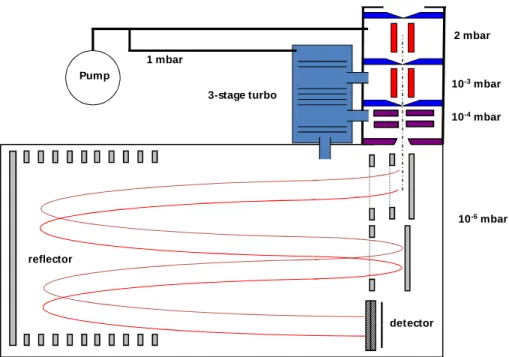
The APi-TOF consists of a time-of-flight mass spectrometer (TOF) coupled to an at-mospheric pressure interface (APi) which guides the sampled ions from atat-mospheric pressure to the TOF while pumping away the gas (Fig. 1). The APi is only an interface to the TOF, and should not be confused with atmospheric pressure ionisation, as the

10

APi-TOF in our context does not by default contain any ionization method.

The APi-TOF has three differentially pumped chambers, the first two containing short segmented quadrupoles used in ion guide mode, and the third containing an ion lens assembly. The flow rate into the instrument is∼0.8 l min−1, regulated by a critical orifice (300 µm) at the instrument inlet. The first chamber is pumped down to ∼5 mbar by

15

a scroll pump which can also be used as the backing pump for the turbo pump. The turbo pump has three stages, each pumping a different chamber as seen in Fig. 1. The final pressure in the TOF is typically 10−6_mbar.

The APi-TOF is manufactured by Tofwerk AG, Thun, Switzerland. It can be config-ured to measure either positive or negative ions, and can be run in either of two modes,

20

V orW, the letters symbolizing the flight path of the ions inside the instrument. With the shorter flight path (V mode) which was used in this study, the resolving power (R) is specified to 3000 Th/Th and the mass accuracy to better than 20 ppm (0.002%). Re-solving power is defined asR=M/∆M, whereM is mass/charge and ∆M is the peak width at its half maximum. The TOF is the same as used in the Aerodyne aerosol mass

25

(5)

AMTD

3, 599–636, 2010

ion composition

H. Junninen et al.

◭ ◮

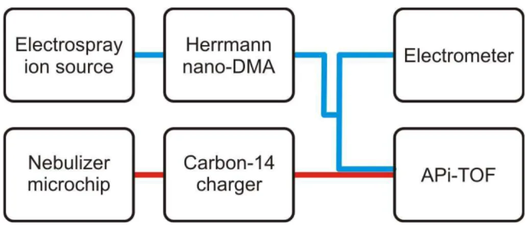
2.2 Laboratory test setups

Two different laboratory setups were used for testing the ion transmission and concen-tration response of the instrument. In the first setup the APi-TOF was connected in parallel with an electrometer, both sampling from a Herrmann nano differential mobility analyzer (HDMA, Herrmann, 2000). It takes advantage of high flow rates (sheath flow

5

rate of up to 2000 l min−1_{and sample flow of 15 l min}−1_{) and can classify ions from 2.15} to 0.02 cm2V−1_s−1_{in electrical mobility corresponding to diameter of 0.8 to 10 nm. The} HDMA has been used previously in conjuction with the aerosol electrometer and com-pared with various air ion spectrometers (Asmi et al., 2009). Ions were produced by electrospraying tetra-alkyl ammonium halides, which are commonly used positive ion

10

mobility standards (Ude and Fernandez de la Mora, 2005).

In the second set-up, the sample was produced with a heated nebulizer microchip (Saarela et al., 2007), which has previously been used in various atmospheric pressure ionization ion sources ( ¨Ostman et al., 2004; Haapala et al., 2007). In this work, a sy-ringe pump introduced a small amount of sample (1–3 µl min−1_{) to a nitrogen flow of}

15

0.3 l min−1_{. The nitrogen flow was heated to 300}◦_{C by an integrated platinum heater.} The mixture was then sprayed through the nozzle of the chip producing a confined plume, which was feed directed into a Carbon-14 beta charger. To decrease losses, a bypass flow of 6 l min−1_{of room air was also drawn through the charger. A schematic} figure of the laboratory measurements performed in this work is shown in Fig. 2, the

20

blue trace corresponding to the first setup, and the red trace to the second.

3 Data analysis

3.1 Mass calibration

Typical data analysis of time-of-flight mass spectrometry data starts with relating the time-of-flight to the mass/charge of the ions. This relation is physically well defined,

(6)

AMTD

3, 599–636, 2010

ion composition

H. Junninen et al.

◭ ◮

but because of instrumental factors and uncertainties in knowing the exact conditions in the ion flight region, it is common to use an empirical calibration function

M=m

Q=

t−b

a 2

(1)

wherem/Qis the mass/charge ratio of the ion,t is the measured ion flight time, anda

andbare instrumental parameters.

5

The mass calibration of a TOF is based on defining the instrumental parameters in Eq. (1) by sampling known substances over a wide range ofm/Q, measuring ion flight times and fitting Eq. (1) to the data. In the laboratory a common practice is to calibrate the TOF before and after the measurement of an unknown sample and assume no change during the experiment. This is in general a good assumption, since the most

10

important external factor that e_ffects the calibration is temperature, which is reasonably constant in the laboratory. However, when measuring in a field station the temperature can fluctuate considerably during a day and this can change the mass calibration.

We developed a tool (tofTools) to post-process long time series of measurements utilizing an unknown sample itself and only having a known calibration occasionally.

15

A similar approach is also used in the analysis of the Aerodyne aerosol mass spec-trometer (AMS) data (De Carlo et al., 2006). However, compared to the AMS, our signals are much lower and an additional averaging prior the calibration is needed. Also, in the AMS all the spectra are very much alike and in every single AMS spec-trum there is always a set of known peaks that can be used for mass calibration. The

20

APi-TOF signal, on the other hand, does not have the virtue of having a constant ion-ization nor constant features in the spectra. The signal changes when the ion balance and/or composition in the atmosphere changes or when the ionization technique in front of the instrument is changed. The software cannot rely on a constant presence of background peaks that could be used for calibration.

(7)

AMTD

3, 599–636, 2010

ion composition

H. Junninen et al.

◭ ◮

TofTools is implemented in the MATLAB (Matlab, version 7.6, R2008a1) environ-ment and features automatic averaging, mass calibration, baseline detection, peak de-convolution and stick calculation. The software is still work in progress and is in beta-development stage. Most of the methods used in tofTools are basic data-analysis techniques and will not be discussed here. However, we find that a robust mass

cali-5

bration of a partly or completely unknown spectrum is a novel feature that is not found in other software packages. Many algorithms are developed for calibration of pep-tide measurements with liquid chromatography TOF (e.g., Jaitly et al. 2006), or with MALDI-TOF (Wolski et al., 2005), but in these cases the second dimension from the chromatographic separation has been utilized. We only have a 1-Ddata.

10

The mass calibration of an unknown spectrum is a multistep process, where several methods are applied before the final solution is reached. The first step is to get a rough mass calibration with an accuracy of at least 0.5 Th. This is often already reached when the instrument is calibrated often enough in the field and the sampling conditions are not changed. If for some reason this is not the case, a rough mass calibration can be

15

achieved by assuming that each peak is roughly at integer mass. After finding all the peaks (or peaks above some threshold) from the spectrum we find values for constants

aandbin Eq. (1) that minimize the average distance of each peak to its integer mass (δ) as in

δ=

s PI

i=1(Mi−Mi)

I , (2)

20

whereM is the integer mass, and M is the peak mass calculated by Eq. (1). TheI

represents the number of peaks in the spectrum.

Now that the rough mass calibration is achieved, one can either search for known peaks and do a traditional mass calibration or proceed with a second step in the cali-bration of the unknown spectrum.

25

1

(8)

AMTD

3, 599–636, 2010

ion composition

H. Junninen et al.

◭ ◮

The second step in the calibrating of an unknown spectrum follows a baseline op-timization. Here we assume that with the optimum values for the instrumental pa-rameters a and b the average of the baseline region over the whole spectrum gives a minimum value. The baseline region is defined as a 0.4 Th wide area between the peaks. The baseline optimization minimizes the equation

5

β=

I

X

i=10 Pi+0.7

p=i+0.3Sp

L_i , (3)

Where β is average of spectral points that belongs to baseline, I is the number of integer masses, S_p represents a spectral point at sampling number p, and L is the number of the spectral points at integer mass i. Note that the number of spectral points is different for each mass, the small masses are sampled at a higher rate due to

10

the relation in Eq. (1).

After this step, unit mass resolution time series are calculated and can be analysed and used to identify different peaks. Once enough peaks are positively identified, these masses can be added to a mass table which is subsequently used to recalibrate the current and future similar spectra with a high mass accuracy.

15

3.2 Peak identification

The APi-TOF by default does not provide any chemical or physical separation prior to sampling as is often done in GC-MS, LC-MS or MS-MS systems. However, due to the high sensitivity, accuracy and mass and time resolution of the APi-TOF, many techniques can be used to determine the elemental and even molecular composition

20

(9)

AMTD

3, 599–636, 2010

ion composition

H. Junninen et al.

◭ ◮

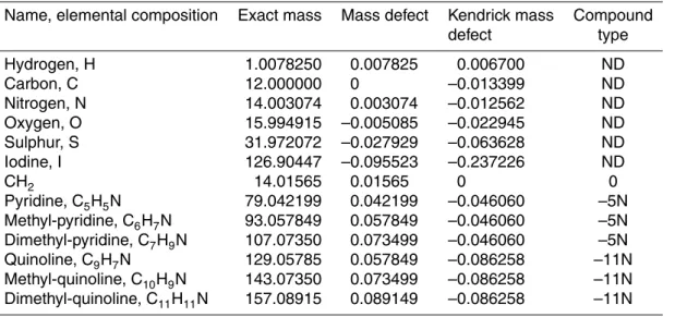
3.2.1 Exact mass and Kendrick analysis

High resolution mass spectrometry does not only give a possibility to separate closely located peaks, but also gives information on the composition of the substrate. The position of a peak compared to its integer mass is called a mass defect and it is de-pendent on the elemental composition of the molecule. When the instrument is well

5

calibrated, the accuracy is less than 20 ppm, leaving few options at masses below 200 Th. Table 1 lists exact masses and the mass defects of some common elements and some selected organic molecules.

Members of hydrocarbon homologous series differ from each other by a mass of CH₂(14.01565 Da). Thus, it is possible to recognise patterns of compounds belonging

10

to the same family by finding a series of peaks differing by 14.01565 Th. It simpli-fies the interpretation of a complex organic mass spectrum by expressing the mass of hydrocarbon molecules in Kendrick units (where m(12CH₂)=14 Ke) instead of Dalton (wherem(12C)=12 Da) (Kendrick, 1963). In Kendrick units all the members of the ho-mologous series have the same Kendrick mass defect (Kendrick mass defect=Kendrick

15

mass−Kendrick nominal mass) (see Table 1) (Hughey et al., 2001; Smith et al., 2009). Based on the di_fference of hydrogen and carbon in heteroatom organic molecules we can classify each molecule CcHhNnOowith an integer numberZ

Z=h−2c, (4)

where h is the number of hydrogen and c is the number of carbon atoms in the

20

molecule. HenceZ reflects the number of rings and double bonds in the molecule. For example a protonated pyridine, C5H6N+ has Z=6–10=−4 and is denoted as

a type−4N and for an aminophenol C6H8NO+, Z=8–12=−4 and is denoted as type

−4NO (Hughey et al., 2001).

If we plot the Kendrick mass defects against the Kendrick nominal masses, all the

25

(10)

AMTD

3, 599–636, 2010

ion composition

H. Junninen et al.

◭ ◮

atoms). This is called a Kendrick diagram. Additionally, when using a known mass accuracy for the instrument we can automatically search for substances that belong to a specific family by searching for the peaks that have a nominal Kendrick mass matching the series, and the Kendrick mass defect is within plus or minus the mass accuracy. Highlighting the discovered peaks greatly aids in identifying the peaks in the

5

mass spectrum. An example of such an analysis is shown in Sect. 4.5.

Before the data is plotted on the Kendrick diagram, one has to determine the ex-act m/Q of the peaks in the spectrum. In tofTools we have implemented a peak fitting routine where Gaussian distributions are used. Compared to standard peak fitting procedures some changes have been implemented: 1) weighting is applied to

10

the negative residuals (over the fitted data points). This modification makes the fitting more robust against skewed peaks, and gives a better estimation of the exact peak location (exact m/Q). 2) Peak area is not fitted, but is calculated by solving nlinear equations (n=number of overlaying peaks) using matrix algebra (Hussein et al., 2005). This speeds up the fitting algorithm considerably, particularly when multiple overlaying

15

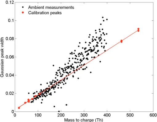
peaks are fitted. 3) The width of the fitted peaks is constrained to a single parameter which is scaled by a linear function of them/Qratio. The dependency of the peak width on them/Q is evaluated from a set of peaks that do not have interefering peaks at the same nominal mass. Here we have used ammonia, isopropanol, butanol, acetone, pinene and two siloxane peaks (462.123 Th and 536.142 Th). All compounds except

20

ammonia were separately added to the sample. The siloxanes are contaminants from conductive tubing and are very easily ionized with a radioactive charger. The width to mass relation is depicted in Fig. 3. The peak width from the fitting without constraining the width is also plotted in the same figure. After 180 Th we can see how the uncon-strained peak fits generate artificially too wide peaks. This makes the determination of

25

(11)

AMTD

3, 599–636, 2010

ion composition

H. Junninen et al.

◭ ◮

At the final stage in the peak fitting routine we minimize a weighted root mean square error of fitted Gaussians compared to measured data with a Matlab built-in optimization function based on the Levenberg-Marquardt algorithm (Marquardt, 1963).

3.2.2 Isotopic patterns

Some elements have more than one stable isotope with fairly high abundance, such

5

as sulphur with the isotopes 32S, 33S and 34S, with abundances of 95.02%, 0.75% and 4.21%, respectively. This can often be used to rule out sulphur when determining the molecular formula for a peak. Other elements that have high abundance stable isotopes and are relevant in the current study are silicon (a common contaminant from conductive tubing) and bromide (calibration substance). Examples of the bromide and

10

sulphur isopic distributions are present in Sects. 4.2 and 4.4, respectively.

3.2.3 Correlation diagrams of the time series

Molecules with the same source have similar time trends, and this becomes a very helpful tool once a long time series is collected. This proved especially useful in identifying the peaks of molecular clusters, with correlation coefficients between

15

monomer/dimer/trimer peaks being very high. An example about the usage is pre-sented in Sect. 4.5.

3.2.4 Other criteria

All of the identified peaks in the ambient negative and positive ion spectra were found to be charged through proton transfer, as shown in Sect. 4, which gives two more tools

20

(12)

AMTD

3, 599–636, 2010

ion composition

H. Junninen et al.

◭ ◮

rule: if a substance is detected at an even integer mass, it will contain an odd number of N if ionization involved a proton transfer.

4 Results

4.1 Comparison with ion mobility standards

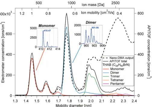
Tetra-heptyl ammonium bromide (THAB) was electrosprayed into a Herrmann DMA,

5

which scanned the mobility range from 0.3 to 1.3 cm2V−1_s−1_{, and the output was} measured by an electrometer and the APi-TOF. The results are depicted in Fig. 4. The electrometer counts all the ions coming out of the HDMA, and this concentration is plotted as the black dashed line in Fig. 4. From previous ion mobility studies (Ude and Fernandez de la Mora, 2005) we know that the peak at mobility diameter 1.47 nm

10

corresponds to the THAB monomer, and the peak at 1.78 nm to the dimer. This was also clearly verified by the APi-TOF.

The horizontal axis in Fig. 4 shows the mass, mobility, and mobility diameter scales. The three different axes are not universally interchangeable, but they are plotted here for reference to show rough relations between three very commonly used quantities.

15

The mass to mobility relationship can be constructed (Ku and Fernandez de la Mora, 2009) since the composition of the THAB clusters are known, and the exact masses can be calculated (and are also measured by the APi-TOF) and the mobility of the clusters has been measured by (Ude and Fernandez de la Mora, 2005). In the same study also the mobility diameter has been calculated up to the THAB pentamer, and

20

this can be used to construct the mass to mobility diameter relationship.

The total ion count seen by the APi-TOF is depicted by the solid black line. Elec-trometer counts are plotted on the left axis, and APi-TOF counts on the right. The other lines correspond to the ion counts related to the di_fferent THAB peaks. As an ex-ample, the most abundant isotope of the tetra-heptyl ammonium cation (THA₊, in the

25

(13)

AMTD

3, 599–636, 2010

ion composition

H. Junninen et al.

◭ ◮

pattern can be found in the monomer inset figure, and the shape is mainly due to the

13

C isotope. Summing up the total signal in the three major isotopes, yields the total monomer signal and this corresponds to the red line in Fig. 4. The dimer consists of a neutral THAB clustered with THA₊, yielding a maximum mono-isotopic mass of 901.86 Da. Bromide has two isotopes of roughly equal abundance at masses 79 and

5

81 Da, and thus the isotopic pattern detected by the APi-TOF is very distinctive as can be seen in the dimer inset figure. Again, summing the signal in all of these peaks yields the total dimer signal, resulting in the light blue line in Fig. 4.

Since we are able to detect THAB clusters up to pentamers, no considerable frag-mentation of the those clusters happened inside the APi-TOF. If this would have been

10

the case, and pentamers and higher clusters would fall apart inside the APi-TOF, we should instead detect the smaller fragments which retained the charge, but this was not the case. This is, however, probably the case with the peak at 1.6 nm which shows up in the APi-TOF as pure monomer although it had a larger size when passing through the HDMA. This implies that it had been clustered with some impurity compound, which

15

was lost before entering the extraction region in the TOF. Losses in the transfer lines were not accounted for, but flow rates were kept high, at 8 l min−1_{and the lines to both} of the instruments were of equal length yielding similar losses.

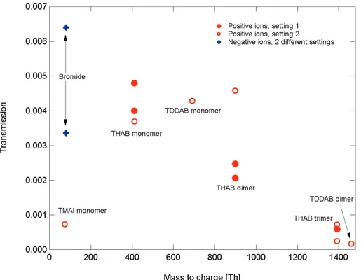
4.2 Transmission

Based on Fig. 4, the APi-TOF signal is roughly a factor of 1000 smaller than the

elec-20

trometer for the monomer and dimer, and this gives an estimate of the transmission of ions from the critical orifice to the detector inside the APi-TOF. For the trimer the trans-mission has decreased slightly, and for the tetra- and pentamers the transtrans-mission has decreased considerably. It should be noted that the electrometer output also becomes more of a continuum after the trimer, possibly due to fragmentation of larger clusters

25

(14)

AMTD

3, 599–636, 2010

ion composition

H. Junninen et al.

◭ ◮

As the losses inside the APi-TOF are m/Q dependent, measurements were con-ducted to map out the transmission curve for the instrument. By transmission, we here mean the fraction of the ions reaching the detector out of the ions reaching the inlet. Thus, it takes into account losses in the inlet, in both of the quadrupoles and in the ion guides, and also the ions passing through the extraction region of the TOF in between

5

extractions (duty cycle).

One way to measure the transmission is to select a monodisperse output from the HDMA and compare the counts in the APi-TOF to those of the electrometer. This was done at several occasions for the THAB monomer-trimer, and with some other tetra-alkyl ammonium halides. The results are shown in Fig. 5. Most of the data is

10

measured in a positive ion mode, as the positive ion mobility standards are much more readily available. Transmission for the smallest mobility standards TMAI at 74 Th and bromide at 80 Th (summed signal of isotopes79Br and81Br) was ranging from 0.07 to 0.64%. The big difference from measurement to measurement is not due to uncertainty in the sampling, but it is the effect of different voltage settings in the APi. Similarly

15

strong dependency on voltage settings was observed on all measured mass ranges, although the difference was the highest with the smallest mass/charge ratio. For THAB monomer (sum over isotopes 410–413 Th) the transmission was from 0.3% to 0.6%, for THAB dimer (sum over isotopes 897–902 Th) the transmission was ranging from 0.2% to 0.5%. The heaviest ion tested (THAB trimer, sum over isotopes 1388–1396 Th) had

20

the transmission of 0.02–0.06%. The final transmission is strongly dependent on the voltage settings in the APi part.

4.3 Concentration response

The response to the changes in concentration seemed to be fairly linear based on the THAB experiments in Sect. 4.1, and this was an assumption we needed to make in

25

order to calculatesm/Qdependent transmissions.

(15)

AMTD

3, 599–636, 2010

ion composition

H. Junninen et al.

◭ ◮

microchip to produce known concentrations of three organic aromatic compounds (ve-rapamil, propanolol and aciridine) that have high proton a_ffinities. We used a14C beta source to charge the sample. When looking at the positive ions in the bi-polar source, a cascade of collisions transfer the charge (proton) to compounds with the highest proton a_ffinities, which were in this case our sample.

5

The response was found to be very close to linear over at least 3 orders of magnitude (Fig. 6) for all three compounds. The ion count per second of the APi-TOF is plotted on the y-axis and the amount of molecules produced by the nebulizer chip ranging from 1×106to 1×1010molec s−1(corresponds to nebulised liquid sample concentration 3×10−2 to 3×102nM) on the x-axis. In the low concentration end, we reached the

10

detection limit of the APi-TOF, which explains the deviation from the linear curve. In the high concentration side, the deviation is most likely due to the charging mechanism, as this comparison assumes that the charged fraction of the compounds is constant. However, the beta charger will always produce a limited amount of charges, and these will start to recombine immediately. Thus, at very high concentrations we expect the

15

amount of ions able to charge the sample to begin to be exhausted and the sample can no longer be ionized to the same extent.

4.4 Sulphuric acid tests

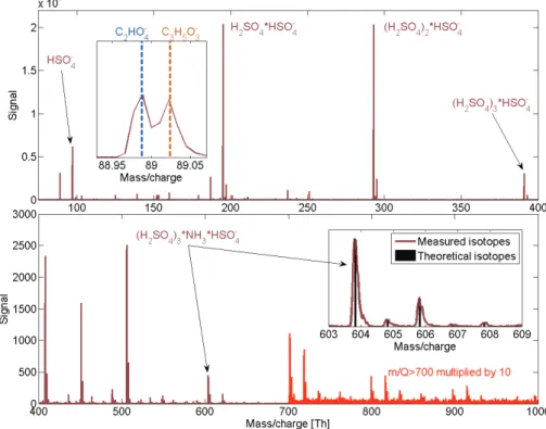
To probe the APi-TOF response to atmospherically relevant test compounds, sulphuric acid (H2SO4) was nebulized with a microchip, and sampled in a similar way as the 20

compounds in Sect. 4.3. The high concentration of H₂SO₄facilitated cluster formation, and the dominant peaks were H2SO4 monomer, dimer, trimer and tetramer (HSO−4,

H2SO4·HSO−4, (H2SO4)2·HSO−4, (H2SO4)3·HSO−4). There was also a very small signal

at the H2SO4pentamer, but starting from the tetramer, the pattern at larger masses was

dominated by clusters of 4 or more H₂SO₄together with ammonia, NH₃ (Fig. 7). The

25

upper panel shows the signal in them/Q range 75–400 Th, and it is dominated by the H2SO4 clusters mentioned above, at integerm/Q 97, 195, 293 and 391. Additionally

there are large peaks at 89 (oxalic acid, HOOC-COO−_{, lactic acid, CH}

(16)

AMTD

3, 599–636, 2010

ion composition

H. Junninen et al.

◭ ◮

and 187 (oxalic acid sulphuric acid cluster, HOOH-COOH·HSO−₄). The first contains two different species, as seen in the inset figure in the top panel of Fig. 7, and is domi-nated by oxalic acid (HOOC-COO−_{), with a shoulder of lactic acid (CH}

3CH(OH)COO−),

whereas the latter is a cluster of oxalic acid with sulphuric acid. The bottom panel de-picts them/Q range 400–1000 Th, with signals abovem/Q700 multiplied by a factor

5

of 10. All the large signals correspond to (H2SO4)m(NH3)nHSO−4 clusters, with a

no-table exception at integerm/Q451 which is a cluster of the H2SO4tetramer and urea

(CO(NH₂)₂, carbonyldiamine). Urea, ammonia and lactic acid are all common con-stituents of sweat (Robinson, 1954), and are also detected in vapours of human skin by on-line electrospray ionization mass spectrometry (Martinez-Lozano and Fernandez

10

de la Mora, 2009), where the set-up used was a very similar to ours. It is therefore not surprising to find these compounds in our laboratory air, however source for oxalic acid is not clear.

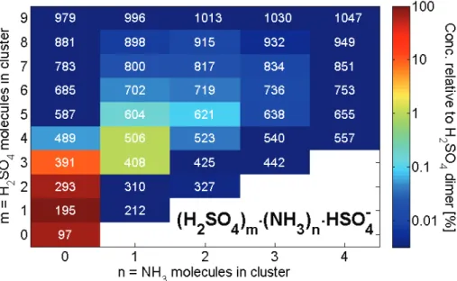
For a better overview, the abundance of all the detected (H2SO4)m(NH3)nHSO−4

clus-ters, where m₌0–9 and n₌0–4, is also plotted in Fig. 8. The color scale is logarithmic,

15

and scaled to the dimer concentration. The numbers in white inside each box shows the integerm/Qat which the cluster was detected. We only detect ammonia in clusters with 4 or more H₂SO₄, which is in fairly good agreement with (Ortega, 2009) who calcu-lated that the addition of ammonia to a sulphuric acid cluster becomes more favourable the more H2SO4 molecules already in the cluster. Also (Hanson and Eisele, 2002) 20

measured (H₂SO₄)_m(NH₃)_nHSO−

4 negative ion clusters and found that ammonia was

abundant in clusters starting from the H2SO4tetramer.

It should be noted that the charging inside the beta source is likely to involve such high energy collisions that almost all the clusters will break apart, and the detected clusters are formed after exiting the charging area. The absolute concentration of

25

H2SO4in this experiment could not be calculated, but it was probably several orders of

magnitude higher than typical daytime ambient concentrations. Nevertheless, we have shown that the APi-TOF can detect these (H2SO4)m(NH3)nHSO−4clusters, and this may

(17)

AMTD

3, 599–636, 2010

ion composition

H. Junninen et al.

◭ ◮

4.5 Ambient data

The concentration of atmospheric ions is usually on the order of 400–2000 ions cm−3 per polarity (Hirsikko et al., 2004). To demonstrate the sensitivity of the APi-TOF, we present ambient air ion data collected at the SMEAR III station in Helsinki, Finland (J ¨arvi et al., 2009). The ambient ions are a subset of the gas phase molecules and

clus-5

ters which have obtained a charge, usually by donating or receiving a proton. Therefore the ions do not accurately represent the whole bulk gas phase composition of the air. The positive ion spectrum will be dominated by the molecules with the highest proton affinities, whereas the negative ion spectrum will be dominated by the anions that have the strongest gas phase acidity. The ambient data was analysed using tofTools as

10

described above.

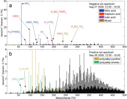
Day time spectra are presented in Fig. 9, for both negative (Fig. 9a) and positive (Fig. 9b) ions. The data is averaged over 6 h. The negative ion spectrum is domi-nated by different inorganic acids, mainly nitric (blue), sulphuric (red) and iodic acid (purple), and their dimers and water clusters. Clusters between the different acids are

15

also visible (brown). While the nitric and sulphuric acid clusters are expected and have been detected before in the ambient negative ion spectrum (Eisele, 1989a; Zhao et al., 2010), iodine compounds have not been previously reported. Figure 10 shows clear correlation between all iodine containing peaks including clusters with sulphuric and nitric acid. This shows the power of using correlograms in ambient data analysis, and

20

the masses could easily be confirmed to contain iodine due to it’s very negative mass defect. Iodine compounds can be abundant in ambient air, particularly in marine and coastal locations (O’Dowd et al., 2002). Negative ion chemical ionization of evapo-rated aerosol particles formed by photo-oxidation of iodine compounds produced mass spectra dominated bym/Q175 (IO−

3) in experiments by (Hoffmann et al., 2001). How-25

(18)

AMTD

3, 599–636, 2010

ion composition

H. Junninen et al.

◭ ◮

The positive ion spectrum is spread out over many more ions than the negative. There are still two distinct groups that can be pointed out, and those are the alkyl amines and the alkyl pyridines. The pyridine series begins with pure protonated pyri-dine, followed by methyl pyripyri-dine, and continues with additions of (CH2)n, with n

reach-ing at least 6. With our instrument we are not able to distreach-inguish between isomers,

5

such as dimethyl pyridine or ethyl pyridine. The amine group follows the same pattern, going from the chemical formula of trimethyl to that of tributyl amine. These peaks still make up only a fraction of the total positive ions detected, and peak identification is still work in progress.

As an example of the mass resolving ability of the APi-TOF, the positive ion mass

10

spectrum at integer mass 130 is plotted in Fig. 11, for the same 6h period as in Fig. 9. Also added to the figure are the 1 h averages, and a fit comprising of two gaussian modes to the 6 h average. The calculated masses for C9H8N+ and C8H20N+ are

plot-ted as dashed lines. The first formula most likely corresponds to protonaplot-ted quinoline, which has been detected already previously by (Eisele, 1989b) in the atmospheric ion

15

population, whereas the second peak could be an alkyl amine, for instance dipropy-lethylamine.

Constraining the peak width according to Fig. 3, we can fit Gaussians to the entire data set and calculate the mass defects and corresponding Kendrick mass defects for each peak. The Kendrick diagram for the positive ions is plotted in Fig. 12. We can

dis-20

tinguish 6 di_fferent compound types instead of the two mentioned above. Four of these can be related to protonated amines (type 4N), protonated pyrrolines (0N), protonated pyridines (−4N) and protonated quinolines (−10N), all with alkyl group additions. Many of these have been detected in the atmosphere previously (Eisele, 1986, 1989b). Clear homologues series are present also for types−6N and −8N, but no chemical

identifi-25

(19)

AMTD

3, 599–636, 2010

ion composition

H. Junninen et al.

◭ ◮

5 Conclusions

In this paper we described the basic principles of the APi-TOF, and tests peformed in the laboratory and in ambient conditions. The transmission of the APi-TOF was de-termined against an electrometer using mobility selected tetra alkyl ammonium halide ions. The transmission was 0.1–0.5% in the range 100–1300 Th, dropping o_ffat both

5

higher and lowerm/Q. It is sensitive to the internal settings, and can be adjusted to maximise the transmission in a desired Th range.

The concentration response was tested with nebulised acridine, propanolol and ver-apamil. The APi-TOF featured a nearly linear response from 107to 1010molec s−1_{. At} the high concentration, the deviation from a linear response is attributed to the fact that

10

the bi-polar ion source was not able to produce enough ions to charge the sampled molecules.

Tests with a high concentration of nebulized sulphuric acid mixed with room air, re-vealed that sulphuric acid readily clusters with itself to form at least pentamers, but at higherm/Qthe ion spectrum was dominated by (H2SO4)m(NH3)nHSO−4 clusters. 15

During this study we developed tools to analyse time series of the mass spectra produced by the APi-TOF. The software package tofTools automatically performs the mass axis calibrations, and produces a high resolution mass spectral time series as well as integrated unit mass spectral time series. One major difference of this soft-ware compared to most other mass spectral analysis tools, is that it is optimized to

20

produce high time resolution, mass calibrated spectra from data with very low signals. From the ambient measurements, we could determine the exact elemental composi-tion of most atmospheric ions up to 200 Th. Above this, we can still efficiently nar-row down the possibilities, but the uncertainty increases as the number of possible molecules and the absolute mass uncertainty at each peak is higher, and a peak is

25

(20)

AMTD

3, 599–636, 2010

ion composition

H. Junninen et al.

◭ ◮

alkyl pyridines. In the negative ion spectrum we detected mostly inorganic acids and their clusters.

The APi-TOF sampled naturally charged ions directly from ambient air without any chemical or electrical manipulation of the sample. It can also be coupled to external chargers and one of our future aims is to develop chemical ionization methods to be

5

able to selectively detect also molecules and clusters that are not usually charged in the atmosphere. Recently Zhao et al. (2010) investigated the composition of neutral clusters using a cluster-CIMS. They used a quadrupole MS with unit mass resolving power coupled to a CI unit. By using NO−

3 or HNO3·NO−3 as a charger ion, they limit

their studies to sulphuric acid and its clusters. By adding a chemical ionization unit to

10

APi-TOF we can use weaker acids as charger ions and thus be less selective, but still able to interpret the mass spectra, due to the high mass accuracy and resolving power of the instrument.

The ultimate purpose of the APi-TOF is to sample molecules and clusters in am-bient air, but also in laboratory and chamber studies. We have showed the

in-15

strument’s ability to measure atmospherically relevant compounds such as charged (H₂SO₄)_m(NH₃)_nHSO−

4 clusters in the laboratory, and these clusters may play a very

important role in aerosol particle formation. We also presented data of ambient natu-rally charged ions, which are typically present at concentrations below 1000 cm−3 _per polarity. Regardless of the low concentrations, the APi-TOF provided clear mass

spec-20

tra of the ions, and a large number of compounds were already identified. In ambient measurements the signals are often very low, and the high sensitivity, accuracy and resolution of the APi-TOF make it a very promising instrument for studies of nucleation and new particle formation.

Acknowledgements. This work has been partially funded by European Commission 6th Frame-25

(21)

AMTD

3, 599–636, 2010

ion composition

H. Junninen et al.

◭ ◮

References

Arnold, F.: Atmospheric ions and aerosol formation, Space Sci. Rev., 137, 225–239, 2008. Arnold, F.: Multi-Ion complexes in the Stratosphere – implications for trace gases and aerosol,

Nature, 284, 610–611, 1980.

Asmi, E., Sipil ¨a, M., Manninen, H. E., Vanhanen, J., Lehtipalo, K., Gagn ´e, S., Neitola, K., 5

Mirme, A., Mirme, S., Tamm, E., Uin, J., Komsaare, K., Attoui, M., and Kulmala, M.: Results of the first air ion spectrometer calibration and intercomparison workshop, Atmos. Chem. Phys., 9, 141–154, 2009,

http://www.atmos-chem-phys.net/9/141/2009/.

De Gouw, J. A. and Warneke, C.: Measurements of volatile organic compounds in the earth’s 10

atmosphere using proton-transfer-reaction mass spectrometry, Mass Spectrom. Rev., 26, 223–257, 2006.

DeCarlo, P. F., Kimmel, J. R., Trimborn, A., Northway, M. J., Jayne, J. T., Aiken, A. C., Gonin, M., Fuhrer, K., Horvath, T., Docherty, K. S., Worsnop, D. R., and Jimenez, J. L.: Field-deployable, high-resolution, time-of-flight aerosol mass spectrometer, Anal. Chem., 78, 8281–8289, 15

2006.

Eisele, F. L.: Identification of tropospheric ions, J. Geophys. Res., 91, 7897–7906, 1986. Eisele, F. L.: Natural and anthropogenic negative-ions in the troposphere, J. Geophys.

Res.-Atmos., 94, 2183–2196, 1989a.

Eisele, F. L.: Natural and transmission-line produced positive-ions, J. Geophys. Res.-Atmos., 20

94, 6309–6318, 1989b.

Fernandez de la Mora, J., Thomson, B. A., and Gamero-Castano, M.: Tandem mobility mass spectrometry study of electrosprayed tetraheptyl ammonium bromide clusters, J. Am. Soc. Mass Spectr., 16, 717–732, 2005.

Haapala, M., Luosujarvi, L., Saarela, V., Kotiaho, T., Ketola, R. A., Franssila, S., and Kos-25

tiainen, R.: Microchip for combining gas chromatography or capillary liquid chromatogra-phy with atmospheric pressure photoionization-mass spectrometry, Anal. Chem., 79, 4994– 4999, 2007.

Hanson, D. R. and Eisele, F. L.: Measurement of prenucleation molecular clusters in the NH₃, H₂SO₄, H₂O system, J. Geophys. Res.-Atmos., 107, 2002.

30

(22)

AMTD

3, 599–636, 2010

ion composition

H. Junninen et al.

◭ ◮

Printer-friendly Version Interactive Discussion Herrmann, W., Eichler, T., Bernardo, N., and Fernandez de la Mora, J.: Turbulent transition

arises at Re 35 000 in a short Vienna type DMA with a large laminarizing inlet, Proceedings of the annual conference of the AAAR, St. Louis, MO, 6–10 October 2000.

Hirsikko, A., Laakso, L., H ˜orrak, U., Aalto, P. P., Kerminen, V.-M., and Kulmala, M.: Annual and size dependent variation of growth rates and ion concentrations in boreal forest, Boreal 5

Environ. Res., 10, 357–369, 2005.

Hoffmann, T., O’Dowd, C. D., and Seinfeld, J. H.: Iodine oxide homogeneous nucleation: an explanation for coastal new particle production, Geophys. Res. Lett., 28, 1949–1952, 2001. Huey, L. G.: Measurement of trace atmospheric species by chemical ionization mass

spec-trometry: Speciation of reactive nitrogen and future directions, Mass. Spectrom. Rev., 26, 10

166–184, 2007.

Hughey, C. A., Hendrickson, C. L., Rodgers, R. P., Marshall, A. G., and Qian, K. N.: Kendrick mass defect spectrum: a compact visual analysis for ultrahigh-resolution broadband mass spectra, Anal. Chem., 73, 4676–4681, 2001.

Hussein, T., Dal Maso, M., Petaja, T., Koponen, I. K., Paatero, P., Aalto, P. P., Hameri, K., 15

and Kulmala, M.: Evaluation of an automatic algorithm for fitting the particle number size distributions, Boreal Environ. Res., 10, 337–355, 2005.

Iida, K., Stolzenburg, M. R., McMurry, P. H., and Smith, J. N.: Estimating nanoparticle growth rates from size-dependent charged fractions: Analysis of new particle formation events in Mexico City, J. Geophys. Res.-Atmos., 113, D05207, doi:10.1029/2007JD009260, 2008. 20

Jaitly, N., Monroe, M. E., Petyuk, V. A., Clauss, T. R. W., Adkins, J. N., and Smith, R. D.: Robust algorithm for alignment of liquid chromatography-mass spectrometry analyses in an accurate mass and time tag data analysis pipeline, Anal. Chem., 78, 7397–7409, 2006.

J ¨arvi, L., Hannuniemi, H., Hussein, T., Junninen, H., Aalto, P. P., Hillamo, R., Makela, T., Kero-nen, P., Siivola, E., Vesala, T., and Kulmala, M.: The urban measurement station SMEAR 25

III: Continuous monitoring of air pollution and surface-atmosphere interactions in Helsinki, Finland, Boreal Environ. Res., 14, 86–109, 2009.

Jayne, J. T., Leard, D. C., Zhang, X. F., Davidovits, P., Smith, K. A., Kolb, C. E., and Worsnop, D. R.: Development of an aerosol mass spectrometer for size and composition analysis of submicron particles, Aerosol Sci. Tech., 33, 49–70, 2000.

30

(23)

AMTD

3, 599–636, 2010

ion composition

H. Junninen et al.

◭ ◮

Printer-friendly Version Interactive Discussion Hueglin, C., Sun, Y. L., Tian, J., Laaksonen, A., Raatikainen, T., Rautiainen, J.,

Vaatto-vaara, P., Ehn, M., Kulmala, M., Tomlinson, J. M., Collins, D. R., Cubison, M. J., Dun-lea, E. J., Huffman, J. A., Onasch, T. B., Alfarra, M. R., Williams, P. I., Bower, K., Kondo, Y., Schneider, J., Drewnick, F., Borrmann, S., Weimer, S., Demerjian, K., Salcedo, D., Cot-trell, L., Griffin, R., Takami, A., Miyoshi, T., Hatakeyama, S., Shimono, A., Sun, J. Y., 5

Zhang, Y. M., Dzepina, K., Kimmel, J. R., Sueper, D., Jayne, J. T., Herndon, S. C., Trim-born, A. M., Williams, L. R., Wood, E. C., Middlebrook, A. M., Kolb, C. E., Baltensperger, U., and Worsnop, D. R.: Evolution of Organic Aerosols in the Atmosphere, Science, 326, 1525– 1529, 2009.

Jordan, A., Haidacher, S., Hanel, G., Hartungen, E., Mark, L., Seehauser, H., Schottkowsky, R., 10

Sulzer, P., and Mark, T. D.: A high resolution and high sensitivity proton-transfer-reaction time-of-flight mass spectrometer (PTR-TOF-MS), Int. J. Mass. Spectrom., 286, 122–128, 2009.

Kendrick, E.: A mass scale based on CH₂₌14.0000 for high resolution mass spectrometry of organic compounds, Anal. Chem., 35, 2146–2154, 1963.

15

Kerminen, V.-M., Pirjola, L., and Kulmala, M.: How signifigantly does coagulation scavening limit atmospheric particle production?, J. Geophys. Res., 106, 24119–24125, 2001.

Ku, B. K. and Fernandez de la Mora, J.: Relation between electrical mobility, mass, and size for nanodrops 1–6.5 nm in diameter in air, Aerosol Sci. Tech., 43, 241–249, 2009.

Kulmala, M. and Kerminen, V. M.: On the formation and growth of atmospheric nanoparticles, 20

Atmos. Res., 90, 132–150, 2008.

Kulmala, M., Riipinen, I., Sipila, M., Manninen, H. E., Petaja, T., Junninen, H., Dal Maso, M., Mordas, G., Mirme, A., Vana, M., Hirsikko, A., Laakso, L., Harrison, R. M., Hanson, I., Le-ung, C., Lehtinen, K. E. J., and Kerminen, V. M.: Toward direct measurement of atmospheric nucleation, Science, 318, 89–92, 2007.

25

Kulmala, M., Vehkamaki, H., Petaja, T., Dal Maso, M., Lauri, A., Kerminen, V. M., Birmili, W., and McMurry, P. H.: Formation and growth rates of ultrafine atmospheric particles: a review of observations, J. Aerosol Sci., 35, 143–176, 2004.

Kulmala, M.: How particles nucleate and grow, Science, 302, 1000–1001, 2003.

Marquardt, D. W.: An algorithm for least-squares estimation of nonlinear parameters, J. Soc. 30

Ind. Appl. Math., 11, 431–441, 1963.

(24)

AMTD

3, 599–636, 2010

ion composition

H. Junninen et al.

◭ ◮

Printer-friendly Version Interactive Discussion Mirme, A., Tamm, E., Mordas, G., Vana, M., Uin, J., Mirme, S., Bernotas, T., Laakso, L.,

Hir-sikko, A. and Kulmala, M.: A wide-range multi-channel air ion spectrometer, Boreal Environ. Res., 12, 247–264, 2007.

O’Dowd, C. D., Jimenez, J. L., Bahreini, R., Flagan, R. C., Seinfeld, J. H., Hameri, K., Pirjola, L., Kulmala, M., Jennings, S. G., and Hoffmann, T.: Marine aerosol formation from biogenic 5

iodine emissions, Nature, 417, 632–636, 2002.

Ortega, I. K., Kurt ´en, T., Vehkam ¨aki, H., and Kulmala, M.: Corrigendum to “The role of ammonia in sulfuric acid ion induced nucleation” published in Atmos. Chem. Phys., 8, 2859–2867, 2008, Atmos. Chem. Phys., 9, 7431–7434, 2009,

http://www.atmos-chem-phys.net/9/7431/2009/. 10

¨

Ostman, P., Marttila, S. J., Kotiaho, T., Franssila, S., and Kostiainen, R.: Microchip atmospheric pressure chemical ionization source for mass spectrometry, Anal. Chem., 76, 6659–6664, 2004.

Saarela, V., Haapala, M., Kostiainen, R., Kotiaho, T., and Franssila, S.: Glass microfabricated nebulizer chip for mass spectrometry, Lab Chip, 7, 644–646, 2007.

15

Sipila, M., Lehtipalo, K., Attoui, M., Neitola, K., Petaja, T., Aalto, P. P., O’Dowd, C. D., and Kulmala, M.: Laboratory verification of PH-CPC’s ability to monitor atmospheric sub-3 nm clusters, Aerosol Sci. Tech., 43, 126–135, 2009.

Sipil ä, M., Lehtipalo, K., Kulmala, M., Pet äj ä, T., Junninen, H., Aalto, P. P., Manninen, H. E., Kyr ö, E.-M., Asmi, E., Riipinen, I., Curtius, J., K ürten, A., Borrmann, S., and O’Dowd, C. 20

D.: Applicability of condensation particle counters to measure atmospheric clusters, Atmos. Chem. Phys., 8, 4049–4060, 2008,

http://www.atmos-chem-phys.net/8/4049/2008/.

Smith, J. N., Dunn, M. J., Vanreken, T. M., Iida, K., Stolzenburg, M. R., McMurry, P. H., and Huey, L. G.: Chemical composition of atmospheric nanoparticles formed from nucleation in 25

Tecamac, Mexico: Evidence for an important role for organic species in nanoparticle growth, Geophys. Res. Lett., 35, L04808, doi:10.1029/2007GL032523, 2008.

Smith, J. N., Moore, K. F., Eisele, F. L., Voisin, D., Ghimire, A. K., Sakurai, H., and Mc-Murry, P. H.: Chemical composition of atmospheric nanoparticles during nucleation events in Atlanta, J. Geophys. Res., 110, D22S03, doi:10.1029/2005JD005912, 2005.

30

(25)

AMTD

3, 599–636, 2010

ion composition

H. Junninen et al.

◭ ◮

Printer-friendly Version Interactive Discussion Tanner, D. J. and Eisele, F. L.: Ions in oceanic and continental air masses, J. Geophys.

Res.-Atmos., 96, 1023–1031, 1991.

Ude, S. and Fernandez de la Mora, J. F.: Molecular monodisperse mobility and mass standards from electrosprays of tetra-alkyl ammonium halides, J. Aerosol. Sci., 36, 1224–1237, 2005. Voisin, D., Smith, J. N., Sakurai, H., McMurry, P. H., and Eisele, F. L.: Thermal desorption 5

chemical ionization mass spectrometer for ultrafine particle chemical composition, Aerosol Sci. Technol., 37, 471–475, 2003.

Wolski, W. E., Lalowski, M., Jungblut, P., and Reinert, K.: Calibration of mass spectrometric peptide mass fingerprint data without specific external or internal calibrants, BMC Bioinfor-matics, 6, 203, doi:10.1186/1471-2105-6-203, 2005.

10

(26)

AMTD

3, 599–636, 2010

ion composition

H. Junninen et al.

◭ ◮

Table 1.Exact masses, mass defects, Kendrick mass defects and compound types for selected elements and molecules.

Name, elemental composition Exact mass Mass defect Kendrick mass Compound

defect type

Hydrogen, H 1.0078250 0.007825 0.006700 ND

Carbon, C 12.000000 0 –0.013399 ND

Nitrogen, N 14.003074 0.003074 –0.012562 ND

Oxygen, O 15.994915 –0.005085 –0.022945 ND

Sulphur, S 31.972072 –0.027929 –0.063628 ND

Iodine, I 126.90447 –0.095523 –0.237226 ND

CH₂ 14.01565 0.01565 0 0

Pyridine, C₅H₅N 79.042199 0.042199 –0.046060 –5N

Methyl-pyridine, C₆H₇N 93.057849 0.057849 –0.046060 –5N Dimethyl-pyridine, C₇H₉N 107.07350 0.073499 –0.046060 –5N

Quinoline, C₉H₇N 129.05785 0.057849 –0.086258 –11N

(27)

AMTD

3, 599–636, 2010

ion composition

H. Junninen et al.

◭ ◮

reflector

detector

10-6_mbar

10-4_mbar

10-3_mbar

2 mbar

3-stage turbo Pump

1 mbar

(28)

AMTD

3, 599–636, 2010

ion composition

H. Junninen et al.

◭ ◮

(29)

AMTD

3, 599–636, 2010

ion composition

H. Junninen et al.

◭ ◮

(30)

AMTD

3, 599–636, 2010

ion composition

H. Junninen et al.

◭ ◮

(31)

AMTD

3, 599–636, 2010

ion composition

H. Junninen et al.

◭ ◮

(32)

AMTD

3, 599–636, 2010

ion composition

H. Junninen et al.

◭ ◮

(33)

AMTD

3, 599–636, 2010

ion composition

H. Junninen et al.

◭ ◮

Fig. 7. Sulphuric acid was nebulized with a microchip and mixed with laboratory air before passing through a beta charger. The dominant peaks in them/Q range below 400 Th (upper panel) are sulphuric acid monomer-tetramer, followed by a peak at integerm/Q89 Th which is most likely a mix of oxalic and lactic acid, as seen in the inset plot. Them/Qrange above 400 Th is dominated by (H₂SO₄)_m(NH₃)_nHSO−

(34)