A simple 2-D inundation model for incorporating flood damage in urban drainage planning

(1)

HESSD

5, 3061–3097, 2008

A simple inundation model for urban

drainage

A. Pathirana et al.

Title Page

Abstract Introduction

Conclusions References

Tables Figures

◭ ◮

Back Close

Full Screen / Esc

Printer-friendly Version

Interactive Discussion

Hydrol. Earth Syst. Sci. Discuss., 5, 3061–3097, 2008 www.hydrol-earth-syst-sci-discuss.net/5/3061/2008/ © Author(s) 2008. This work is distributed under the Creative Commons Attribution 3.0 License.

Hydrology and Earth System Sciences Discussions

Papers published inHydrology and Earth System Sciences Discussionsare under

open-access review for the journalHydrology and Earth System Sciences

A simple 2-D inundation model for

incorporating flood damage in urban

drainage planning

A. Pathirana1, S. Tsegaye2, B. Gersonius1, and K. Vairavamoorthy1

1

UNESCO-IHE Institute for Water Education, P.O. Box 3015, 2601 DA Delft, The Netherlands 2

Bahir Dar University, Engineering Faculty, Bahir Dar, Ethiopia

Received: 1 September 2008 – Accepted: 5 September 2008 – Published: 14 November 2008

Correspondence to: A. Pathirana ([email protected])

(2)

HESSD

5, 3061–3097, 2008

drainage

A. Pathirana et al.

Title Page

Tables Figures

◭ ◮

Back Close

Full Screen / Esc

Abstract

In this paper a new inundation model code is developed and coupled with Storm Wa-ter Management Model, SWMM, to relate spatial information associated with urban drainage systems as criteria for planning of storm water drainage networks. The prime objective is to achive a model code that is simple and fast enough to be consistently

5

be used in planning stages of urban drainage projects.

The formulation for the two-dimensional (2-D) surface flow model algorithms is based on the Navier Stokes equation in two dimensions. An Alternating Direction Implicit

(ADI) finite difference numerical scheme is applied to solve the governing equations.

This numerical scheme is used to express the partial differential equations with time

10

steps split into two halves. The model algorithm is written using C₊₊computer

pro-gramming language.

This 2-D surface flow model is then coupled with SWMM for simulation of both pipe flow component and surcharge induced inundation in urban areas. In addition, a dam-age calculation block is integrated within the inundation model code.

15

The coupled model is shown to be capable of dealing with various flow conditions, as well as being able to simulate wetting and drying processes that will occur as the flood flows over an urban area. It has been applied under idealized and semi-hypothetical cases to determine detailed inundation zones, depths and velocities due to surcharged water on overland surface.

20

1 Introduction

Two-dimensional (2-D) models have been developed for discretising spatial information in flood modeling. Although these existing models can successfully be used for many

flood studies, most of them require much time to simulate different scenarios in urban

areas. However, in planning of urban drainage a simple and quick prediction of flood

25

(3)

HESSD

5, 3061–3097, 2008

drainage

A. Pathirana et al.

Title Page

Tables Figures

◭ ◮

Back Close

Full Screen / Esc

taking hydrodynamic simulation.

This work develops a simple 2-D inundation model code for quick prediction of flood plain hydraulics in urban area. This new 2-D inundation model is then coupled with the 1-D-SWMM for simulation of surcharge induced inundation in urban areas. The coupled model result can be used for further assessment of flood damage costs as a

5

tool for decision in urban drainage planning.

This paper describes how the 2-D model code formulation is done based on Naviers stokes equation and how coupling of the two models is carried out. The performance of the coupled model is also examined for several hypothetic conditions and its application is demonstrated using a semi hypothetical case in Brazil.

10

2 2-D inundation model code development

The inundation model is developed based on the Navier Stokes equation in 2-D. Some-times these equations are also called shallow water equations (SWE). The model for-mulation is done using equations that describe depth average 2-D flow.

The assumption of a 2-D flow over inundated plain as slow, shallow phenomena can

15

reduce the reproduction of flood plain hydraulics to the minimum necessary to achieve acceptable predictions. This simplification may lead to local inaccuracies but many scholars have shown that the uncertainties over the specification of topography and boundary roughness are dominant and thus influence the model results to a greater extent than those incurred through simplified mathematics (Hunter et al., 2007).

20

2.1 Model formulation

(4)

HESSD

5, 3061–3097, 2008

drainage

A. Pathirana et al.

Title Page

Tables Figures

◭ ◮

Back Close

Full Screen / Esc

2.1.1 Governing equations

Continuity equation

The continuity equation for the flood plain flows is formulated using the average flow velocities as a dependent variable. This form of continuity equation can be derived for

unit width of flow where Area=d×1 and has the form shown below. Assuming that the

5

depth of the water doesn’t vary within a time step along horizontal axes, the continuity equation for depth averaged shallow water can be written as:

∂h ∂t +d

_∂u

∂x + ∂v ∂y

=q (1)

Wherehis water stage over the datum which isb+d

d is the depth of flow

10

uandvare velocity components along x- and y-axes, repectively

qis source or sink per unit area

tis flow time

Momentum equation

15

According to Hunter et al. (2007) varied flood flow models can be constructed, depend-ing on which terms in the governdepend-ing equations are assumed negligible. The velocity of the water flow in urban flood plains is very small compared to the other terms. Hence, the convective acceleration term can be ignored and the momentum equation can be written as:

20

∂u ∂t +g

∂h

∂x +gSf x=0 (2)

∂v ∂t +g

∂h

(5)

HESSD

5, 3061–3097, 2008

drainage

A. Pathirana et al.

Title Page Abstract Introduction Conclusions References Tables Figures ◭ ◮ ◭ ◮ Back Close

Full Screen / Esc

WhereS_{f x} andS_{f y} are the friction slopes along x- and y-direction, respectively.

Calculation of friction terms

In this model, the friction termsSf xandSf y are estimated by using the empirical resis-tance relationship in Manning’s equation as follows:

S_{f x}= n 2

upu2₊_v2

d4/3 (4)

5

S_{f y} = n 2

vpu2₊_v2

d4/3 (5)

Wherenis the Manning’s roughness coefficient.

2.1.2 Numerical model

The numerical method that is implemented for the model formulation is finite difference

method. This method involves discretization of time and space to transform the PDEs

10

to difference equations. The spatial discretization is based on a regular Cartesian grid

and the temporal discretization is based on a uniform time step∆t=tn+1−tn,n=0, 1, 2, 3...

Using temporal and spatial discretization the following equations are obtained from Eq. (1).

15

∂hi ,j ∂t =



 _d

i−1,j+di ,j

2∆x

ui−1,j −

_d i ,j+di+1,j

2∆x

ui ,j

+di ,j2−∆y1+di ,j

vi ,j₋1−

_d i ,j+di ,j+1

2∆y

vi ,j



+q (6)

hn+_{i ,j}1= ∆t



 _d_i

−1,j+di ,j

2_∆x

un_i₋+₁1_,j ₋di ,j+di+1,j

2_∆x

un_{i ,j}+1

+di ,j−1+di ,j

2∆y

v_{i ,j}n+₋1₁₋di ,j+di ,j+1

2∆y

v_{i ,j}n+1



(6)

HESSD

5, 3061–3097, 2008

drainage

A. Pathirana et al.

Title Page

Tables Figures

◭ ◮

Back Close

Full Screen / Esc

Using Eqs. (2) and (3) the rate of change of velocity in x- and y-directions are written as:

∂ui ,j ∂t =−g

∂hi ,j

∂x −gSf x=−g

hi+1,j−hi ,j

∆x

!

−gSf x (8)

∂v_{i ,j} ∂t =−g

∂h_{i ,j}

∂y −gSf y =−g

h_i₊₁_,j₋h_{i ,j}

∆y

!

−gS_{f y} (9)

The above equation can be further simplified by writing the value ofgS_f in term of the

5

dependent variable velocity component.

∂u_{i ,j} ∂t =−g

∂h_{i ,j}

∂x −gSf x=−g

h_i₊1,j−hi ,j ∂x

!

−uS_x (10)

∂v_{i ,j} ∂t =−g

∂h_{i ,j}

∂y −gSf y =−g

h_i₊1,j−hi ,j

∆y

!

−gSy (11)

WhereSx=gn

2√

u2_+v2

d4/3 ;Sy=

gn2√u2_+v2

d4/3

Therefore using Eqs. (10) and (11) the velocity at the next time stepn+1 in x-direction

10

can be written as:

un_{i ,j}+1=−g∆t

∆x

hn_i++₁1_,j −h_{i ,j}n+1−un_{i ,j}(1₋Sx) (12)

Similarly for the velocity along the y-direction

v_{i ,j}n+1=−g∆t

∆x

(7)

HESSD

5, 3061–3097, 2008

drainage

A. Pathirana et al.

Full Screen / Esc

The discretized form of the governing equations which are shown in Eqs. (7), (12) and (13) can be combined to determine the water stage above the datum.

hn+1

i ,j =∆t

       

−₂g_∆∆xt2 di₋1,j+di ,j

h_{i ,j}n+1+₂g_∆∆_xt2 di₋1,j+di ,j

hn+_i₋₁1_,j+di−1,j+di,j

2∆x

un_i₋₁_,j(1₋S_x)

+₂g_∆x∆t2 di ,j+di+1,j

hn+_i₊₁1_,j₋g∆t

2∆x2 di ,j+di+1,j

hn+_{i ,j}1₋di,j+di+1,j

2∆x

un_{i ,j}(1₋S_x)

−₂g∆t_∆y2 di ,j+di ,j₋1

hn_{i ,j}+1+₂g∆t_∆y2 di ,j+di ,j₋1

hn_{i ,j}+₋1₁+di,j+di,j−1

2∆y

v_{i ,j}n₋₁ 1₋S_y +₂g∆t_∆y2 di ,j+1+di ,j

hn_{i ,j}+₊1₁₋g∆t

2∆y2 di ,j+1+di ,j

hn_{i ,j}+1₋di,j+1+di,j

2∆y

v_{i ,j}n 1₋S_y        

+hn_{i ,j}+q∆t

Simplifying the above equation and bringing the hn+_{i ,j}1 terms together, the combined

governing equation will be written as:

5

"

g∆t2

di₋1,j+2di ,j +di+1,j 2∆x2

!

+ di ,j−1+2di ,j +di ,j+1

2∆y2

!!

+1

#

hn_{i ,j}+1

= ∆t

        g∆t

2_∆x2(di₋1,j +di ,j)hni−+11,j+

_d i−1,j+di ,j

2∆x

un_i₋₁_,j(1−Sx)

+₂g_∆∆_xt2(di ,j +di+1,j)h

n+1

i+1,j−

_d i ,j+di+1,j

2_∆x

un_{i ,j}(1−S_x)

+₂g_∆∆_yt2(di ,j +di ,j−1)h

n+1

i ,j−1+

_d_{i ,j}₊_d_{i ,j}

−1

2∆y

v_{i ,j}n₋₁(1₋S_y)

+₂g_∆∆_yt2(di ,j+1+di ,j)h

n+1

i ,j+1−

_d_{i ,j}

+1+di ,j

2∆y

v_{i ,j}n (1₋S_y)

       

+hn_{i ,j} +q∆t (14)

At any time steps the above equation leads to a set of tridigonal system of linear al-gebraic equations which can be solved by forward sweep and a backward substitution. The algorithm is simply Gaussian elimination. The tridiagonal system, which is a

diag-10

onal matrix, along x-axis may be written as:

aa h_i₋1,j +bb hi ,j +cc hi+1,j =d d

wherei andj are row and column counters (0, 1, 2...)

aa,bb,cc anddd are coefficients of linear equation as a function of variableh. Note that:aa_o,cc_i_max₋₁andcc_j_max₋₁have to be zero to form the diagonal matrix.

(8)

HESSD

5, 3061–3097, 2008

drainage

A. Pathirana et al.

Title Page

Tables Figures

◭ ◮

Back Close

Full Screen / Esc

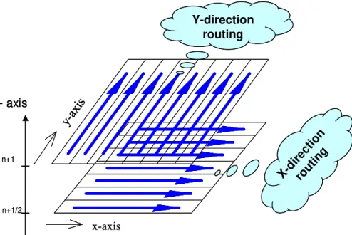
2.1.3 Alternating direction implicit (ADI) finite difference method

In this paper, an alternating direction implicit finite difference (ADI) procedure is used

to solve the governing equations. According to Peaceman and Rachford (1954), the

method provides greater superiority to the explicit finite di_fference method due to high

computational efficiency which requires less computing time because it involves a

tridi-5

agonal matrix. However, this method is not unconditionally stable (Caviglia and Dra-gani, 1996). Consequently Courant condition is applied to reduce possible instabilities in our model.

ADI method is based on splitting the differential equation in two parts. Therefore the

equations are solved sequentially in x- and y-directions in two half time stepstn+1/2

10

andtn+1, respectively: wherenis time step counter.

Simple diagrammatical representation of an alternating direction routing procedure for one full time step is shown in Fig. 1.

Along the x-direction

From time step nton+1/2 the solution for water stage hn+1/2 terms along the x-axis

15

are determined implicitly within a row while the value of other terms are expressed explicitly.

Thus, the values forhn_{i ,j+}+1₁ andhn_{i ,j}+₋1₁are approximated from the previous time step valueshn_{i ,j}₊₁andhn_{i ,j}₋₁respectively. Then Eq. (14) can be further simplified to tridiag-onal set of equation which has the form shown below:

20

(9)

HESSD

5, 3061–3097, 2008

drainage

A. Pathirana et al.

Full Screen / Esc

where

aa=−₂g∆t_∆_x22 di₋1,j +di ,j

bb=g∆t2di−1,j+2di ,j+di+1,j

2∆x2

+di ,j−1+2di ,j+di ,j+1

2∆y2

+1

cc=−₂g_∆∆_xt22 di ,j+di+1,j

d d = ∆t

     _d i−1,j+di ,j

2∆x

un_i₋₁_,j(1−Sx)−

_d i ,j+di+1,j

2∆x

un_{i ,j}(1−Sx)

+₂g∆t_∆y2 di ,j+di ,j₋1

hn_{i ,j}₋₁+di ,j2+d∆yi ,j−1

v_{i ,j}n₋₁ 1−Sy

+₂g∆t_∆_y2 di ,j+1+di ,j

hn_{i ,j+}₁−di ,j+1+di ,j

2∆y

v_{i ,j}n 1−S_y 

   

+hn_{i ,j}+q∆t

along the y-direction (for the next half time step).

During the next time step fromn+1/2 ton+1 the procedure is reversed so that the

5

value ofhalong y-direction is determined implicitly while the other terms are expressed

explicitly and then the water depths are updated from the calculatedhvalues.

Analogues to the x-direction, in case of the y-direction the values forhn_i++₁1_,j andhn_i₋+₁1_,j are approximated from the previous half time step valueshn+_i+₁1_,j/2 and hn+_i₋₁1_,j/2, respec-tively, and Eq. (14) can be converted to linear algebraic equation shown below:

10

aa hn+1

i ,j₋1+bb h

n+1

i ,j +cc h n+1

i ,j+1=d d (16)

Where

aa=−₂g∆t_∆_y22 di ,j +di ,j−1

bb=g∆t2di−1,j+2di ,j+di+1,j

2_∆x2

+di ,j−1+2di ,j+di ,j+1

2_∆y2

+1

cc=−₂g∆t_∆y22 di ,j+1+di ,j

(10)

HESSD

5, 3061–3097, 2008

drainage

A. Pathirana et al.

Title Page

Tables Figures

◭ ◮

Back Close

Full Screen / Esc

d d = ∆t



   

g∆t

2∆x2 di−1,j+di ,j

hn_i₋+₁1_,j/2+di−1,j+di ,j

2∆x

un_i₋₁_,j(1₋Sx)

+₂g_∆x∆t2 di ,j +di+1,j

hn_i++₁1_,j/2−di ,j+di+1,j

2∆x

un_{i ,j}(1₋Sx)

+di ,j2+d∆yi ,j−1

v_{i ,j}n₋₁ 1₋Sy

−di ,j+1+di ,j

2∆y

v_{i ,j}n 1₋Sy



   

+hn+_{i ,j}1/2+q∆t

After computing the value ofh, the velocity components along the x- and y-directions

will be updated by implementing Eqs. (12) and (13), respectively.

2.2 Courant condition

According to Caviglia and Dragani (1996) the ADI numerical scheme is not

uncondi-5

tionally stable when applied to the complete set of governing equations in an area with real topography and irregular boundaries. The instability arises because the routing method uses implicit values along one direction while the values in the orthogonal di-rection are determined explicitly from the previous time step. Thus courant limitation in

time step∆tis implemented to ensure the necessary stability during simulation.

10

|u|+pgd

∆x +

|v|+pgd

∆y

!

∆t≤1 (17)

where∆t is the finite difference time step,∆x and∆y are the regular grid spacings in

the x- and y-directions, respectively, andd is the water depth.

In this inundation model the time step is defined as an input parameter and it has

to be less than the courant∆t for each routing step. During each step of routing the

15

minimum courant_∆t of all cells in the 2-D domain, is calculated using Eq. (17) and

used for verifying the input∆t value.

2.3 Initial and boundary conditions

(11)

HESSD

5, 3061–3097, 2008

drainage

A. Pathirana et al.

Title Page

Tables Figures

◭ ◮

Back Close

Full Screen / Esc

– The initial water depth and velocities terms are taken as zero value over the whole

flood plain area. However, none zero values can be taken as an initial condition.

– Velocity components of the boundary cells are taken as zero value for every time

step.

– On the boundary along the periphery of the area the inflow is set to zero. This is

5

done by modifying the boundary cell equations in such a way that it excludes the outer domain.

2.4 Process representation for wetting/drying cells

In this model the hydraulic parameters are represented for a centroidal point of each cell. However partially wetted cells i.e. cells without enough water to submerged all

10

corners of the cell, the average depth are badly represented by depth at the centroid (Begnudelli and Sanders, 2006). Especially for a cell having very small water depth, the incidence of dry/wet condition will be very high. Therefore, a threshold value of

depthdmin=0.0001 m is propose for classifying submerged cells and updating hydraulic

parameters.

15

One of the reasons of putting a boundary value for minimum depth is to avoid the possible numerical instability of the model. The instability caused by the small depth is due to the fact that the friction terms are computed by dividing with the depth values.

During each full time step the water depth is checked and the velocity and friction

terms of those cells with depth less than dmin are set to zero value to avoid

instabil-20

ity. In addition to the above limiting conditions, depth scaled factor for the Manning’s coe_fficientnmodified=n×dmin

d

(12)

HESSD

5, 3061–3097, 2008

drainage

A. Pathirana et al.

Title Page

Tables Figures

◭ ◮

Back Close

Full Screen / Esc

2.5 Process representation for flow barrier

Features like roads, buildings and dykes have great effect on flow dynamics and flood

propagation. These barriers cause numerical instability in most of the hydrodynamic models. In this model code, the flow interaction near topographic obstacles (barriers) is treated in such a way that an obstacle cell will not contribute to the velocity calculation

5

of the nearest lower cell till it acquires a threshold depth of waterd=0.01 m.

In addition to the velocity calculation, the coe_fficients of the linear algebraic equation for flood flows (Eqs. 15 and 16) are modified for cells that are next to the barrier. The

water stage term of the elevated cell in the coefficient equation of the lowest cell is

replaced by the water stage value of the cell it self to avoid the numerical instability of

10

the model, and to avoid unreasonable flow of water from barrier cells to any neighboring cells.

2.6 Flood damage analysis block

Inundation models help decision makers to have a good perception about the flood

extent and to identify the effective flood mitigation measures through flood risk

assess-15

ment. Therefore a simple damage calculation block is integrated within the inundation model code. The maximum flood depth at each grid cell is used for the calculation of the damage in urban areas. The velocity of the water flow in urban flood plains is very small and it contribution is neglected in the calculation of flood damages. A general equation for the possible flood damage curves is implemented in the model code. This

20

equation is shown below.

Damage=A+BLn(d)+CLog(d)+Dd +E d2+F d3

whered is the flood depth andAtoF are the consecutive coefficients for the possible

flood damage curves. The damage analysis is performed if an input for the damage calculation block is provided.

(13)

HESSD

5, 3061–3097, 2008

drainage

A. Pathirana et al.

Title Page

Tables Figures

◭ ◮

Back Close

Full Screen / Esc

3 Model coupling

There are different frameworks that can be used for model coupling. According to

Bulatewicz (2006), they can be organized into four different categories of coupling

approaches: monolithic, scheduled, communication, and component. In this paper, a communication approach is used for coupling the 2-D-Inundation model with

1-D-5

SWMM. This coupling approach allows existing models to be coupled with minimal changes to the model source codes.

3.1 Creating a coupled model

The sewer overflow is taken as the main interacting physical process between the two selected models. This physical process usually occurs at the point where outfall and

10

surcharged manholes are located. The variables which are integrated in the interacting physical process are

– Routing and reporting time step length

– Duration of simulation

– Overflow volume

15

– Time of occurrence and duration of flooding

The following functions are devised for developing a relationship between variables and incorporated in the main simulating engine of the 2-D model.

– The initialization of both models takes place at the start of simulation. The

inun-dation model routing starts when the manholes begin overflowing. Delaying the

20

flood routing process increases the e_fficiency of this coupled model.

– One of the coupling functions receives overflow information and transforms it into

(14)

HESSD

5, 3061–3097, 2008

drainage

A. Pathirana et al.

Title Page

Tables Figures

◭ ◮

Back Close

Full Screen / Esc

– Because of the coarser time step in SWMM, the inundation model steps a number

of times for a single SWMM report step.

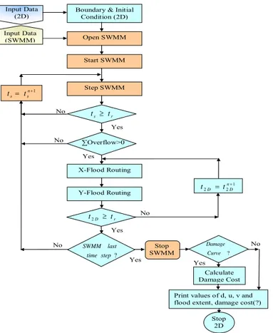
3.2 Coupled model algorithm

The model algorithm, which is used for surface flow routing and flood damage

calcu-lation, is written in C++computer programming language. The simplified algorithm is

5

shown in Fig. 2.

4 Hypothetical test

The flow process representations and simplifications used in this model are checked against the following issues:

– Mass conservation;

10

– Stability and

– Stationary of the result for executions under same condition.

Several hypothetic test problems were utilized to examine the hydrodynamic behavior,

such as boundary conditions, 2-D flood wave diffusion, cell drying and wetting, and

flow interaction with topographic obstacles. Hypothetical examples allow quick visual

15

inspection of the code’s sensitivities and its performance against the simplifications made in the model code.

4.1 Model performance for boundary conditions

The numerical equation in this model is formulated in such a way that no inflow will oc-cur through the boundary cells. Several hypothetical tests were conducted for checking

20

(15)

HESSD

5, 3061–3097, 2008

drainage

A. Pathirana et al.

Title Page

Tables Figures

◭ ◮

Back Close

Full Screen / Esc

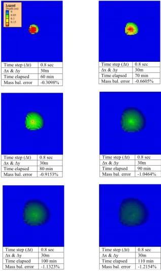
4.2 Model performance against mass balance error

The calculation of mass balance error as percentage (%) of inflow volume to the 2-D

computational domain is done by the model and it can be checked at different instants

of simulation.

massbal=Twdepth−Tsource

Tsource ×100

5

Where massbal is the mass balance error in %, Tsource is the total input volume derived from 1-D simulation and Twdepth is the total volume in 2-D grid domain at same time of simulation.

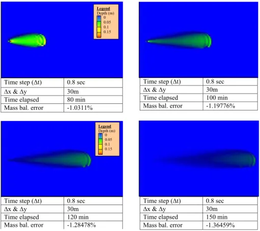
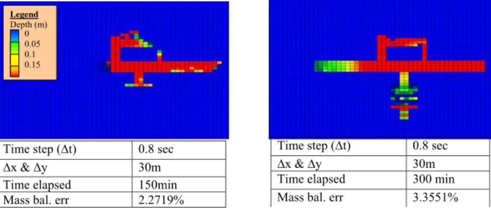
The mass balance of the model is checked for different hypothetical terrains. The

test results for flat, sloping and complex topographies are illustrated in Fig. 3.

10

The above hypothetical tests show that the model produces some mass balance error in the process of flood routing. This error is higher in case of complex topography and long hour simulation as illustrated in Fig. 3. The presence of mass-balance errors in flood flow is a well-known problem, and improving the accuracy and mass-balance properties of fluid flow in general is an active area of research (Kippe et al., 2007).

15

One of the reasons for the mass balance error in the model output is the routing method (Alternating Direction Implicit method). This method uses values from the pre-vious time step of simulation in one direction while implicitly routing in the orthogonal direction.

In addition, a number of simplifications are made to avoid frequent insatiability of the

20

model. The modifications of the numerical equation also create some mass balance error.

4.3 Model performance in wetting and drying problems

The model was examined over hypothetical topography with the various flow conditions that may occur in actual floodplains, such as wetting and drying processes that will

(16)

HESSD

5, 3061–3097, 2008

drainage

A. Pathirana et al.

Title Page

Tables Figures

◭ ◮

Back Close

Full Screen / Esc

occur as the flood flows over an urban area. In this model the wetting/drying process representation is made using a threshold value for water depth. This representation has the advantage listed below:

– Avoids possible numerical instabilities due to very small water depth values.

– Reduce the contribution of partially wetted cells to the neighboring cells.

5

In this test it is also observed that the representation of wetting/drying process creates small inaccuracy in mass balance. However, for the reason that our objective relies on developing a simplified modeling tool, it is reasonable to accept the inaccuracies incurred due to wetting/drying process representation.

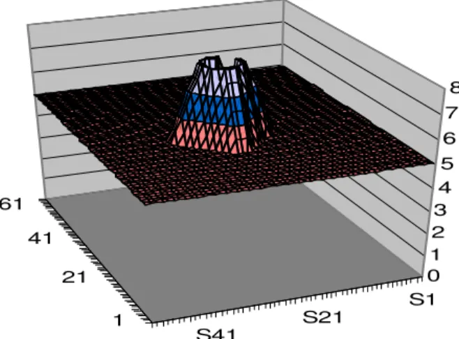
4.4 Model performance in uneven topography including flow barriers

10

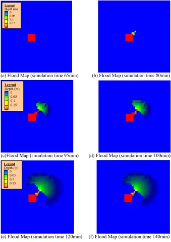
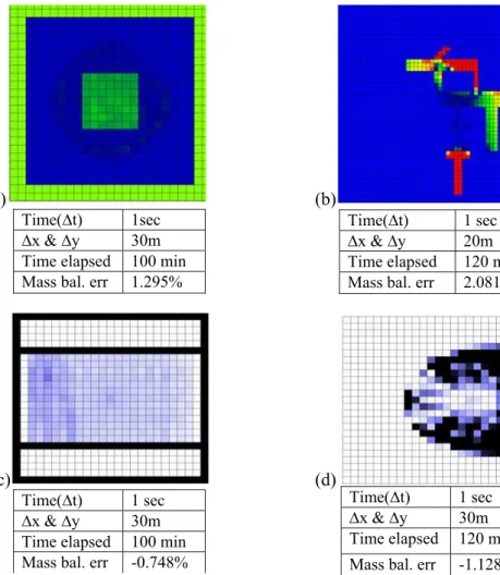
The performance and appropriateness of the flow barrier representations implemented in the model code is examined using an idealized topography. The inundation maps for some hypothetical terrains involving flow barriers are presented in Figs. 4, 5, and 6.

In the above hypothetic test, flood wave diffusion is visually inspected for irregular

terrain shown in Fig. 4. The flood maps at di_fferent times of simulation demonstrate how

15

the flood propagates over the chosen hypothetical topography. The other hypothetical terrains which are used for testing the model are shown in figure below.

For problems involving large flow barriers, the flood wave di_ffusion is visually

in-spected for several synthetic terrains and the numerical model works properly. How-ever, analogous to wetting/drying process, the flow barrier representations

imple-20

(17)

HESSD

5, 3061–3097, 2008

drainage

A. Pathirana et al.

Title Page

Tables Figures

◭ ◮

Back Close

Full Screen / Esc

5 Semi-hypothetical application for case in Brazil, Porto Algere

5.1 Input data’s for the coupled model

5.1.1 Rainfall data

In this case study a 50 year return period, 2hr design rainfall event shown in Fig. 11 is considered for analysis of flooding in the area.

5

5.1.2 Topography

Delineation of the model domain for 2-D computation can be challenging because the modeler doesn’t know the region of inundation before execution (Begnudelli and Sanders, 2007). The approach adopted here was to delineate a boundary significantly far from the flooded manholes.

10

ASCII topographic date for the selected flood plain was downloaded from online site Shuttle Radar Topographic Mission (SRTM) and converted to Raster and geo refer-enced using GIS. Street, building and other flow barrier information’s are added to the terrain to represent urban topography precisely.

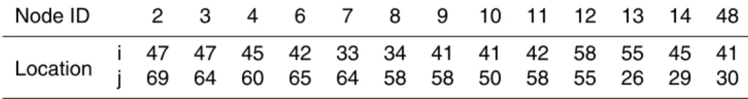
5.1.3 Node locations within 2-D calculation domain

15

There are only 13 nodes within the domain of the selected flood plain area. The

loca-tions based on grid counters (i , j) along x- and y-direction are shown below.

5.1.4 Flood damage data

The input data to be used for the damage analysis was provided by Nascimento et al. (2006).

20

D=130.9+56.3ln(d) whereDis damage cost in Brazilian real currency per m2andd

(18)

HESSD

5, 3061–3097, 2008

drainage

A. Pathirana et al.

Title Page

Tables Figures

◭ ◮

Back Close

Full Screen / Esc

The input required for damage calculation block of the coupled model is the

co-e_fficients associated with the possible stage-damage function. Therefore, A=130.9,

B=56.3 and the other coefficients will be zero.

5.2 Simulation result

As per the simulation result of the existing system, the overflow occurs at a number

5

of manholes. The distribution of flood volume in some of the manholes is shown in Fig. 13.

The coupled model simulation is performed to see the spatial and temporal variation of flood flows. A time step of 1 s and grid size of 20 m are used for this case study. The inundation model generates flood map based on water depth. The flood map at the

10

end of simulation is shown in Fig. 15.

In addition to the flood map, the coupled model prints the velocities in each direction, the flood depths for each grid cells, the flood extent and monetary value of the flood damage on a text file. From the output, it is observed that the model performs well on an irregular topography containing large flow barriers i.e. buildings and it is also

15

examined that it performs well against stability.

6 Conclusions

In this study, development of a new 2-D inundation model code is carried out in C₊₊

computer programming language. The model is then coupled with 1-D-SWMM to simu-late surcharge induced inundation in urban areas and to resimu-late the spatial information’s

20

in design of urban drainage network. Due to the high computational e_fficiency of ADI

numerical scheme, the model also achieves an advantage in required hydrodynamic simulation time.

The 1-D–2-D coupled model was examined over several hypothetical terrain condi-tions, including large flow barriers, sloppy terrains and irregular topography. It is found

(19)

HESSD

5, 3061–3097, 2008

drainage

A. Pathirana et al.

Title Page

Tables Figures

◭ ◮

Back Close

Full Screen / Esc

that the model performs well against stability and stationary result. The model has also been shown to be capable of dealing with the various flow conditions that may occur in actual floodplains, as well as being able to simulate wetting and drying processes that will occur as the flood flows over an urban area. Despite its performance against stability, the model generates small mass balance error.

5

The mass balance error is incurred due to many reasons. One of these reasons is ADI method uses values from the previous time step of simulation in one direction while routing implicitly in the orthogonal direction. Therefore this mechanism of routing by it self introduces small mass balance error in the model output. In addition to this fact, some simplifications and modifications are also made on the numerical equation

10

to avoid frequent insatiability of the model. The modifications will have a possibility to add up the mass balance error but for the reason that our objective relies on developing a simplified modeling tool, it is reasonable to accept those small inaccuracies incurred due to the process representations.

The 1-D–2-D coupled model is applied for case study to determine the detail

inunda-15

tion zones, depths and velocities due to surcharged water. It is also examine for some of the important hydrodynamic behavior, such as boundary conditions, 2-D flood wave propagation, cell drying and wetting, and flow interaction with topographic obstacles. Since the inundation model is based on detailed spatial information i.e. land use and topography, its output will be more realistic to determine flood damage. The flood

dam-20

age calculation block is integrated within the inundation model code. This tool can help flood control authorities to make quick decision on flood damages control measures as a decision support system.

In planning of urban drainage a simple and fast prediction of flood within an accept-able level of error is much more useful and can lead to better understanding of the

25

(20)

HESSD

5, 3061–3097, 2008

drainage

A. Pathirana et al.

Title Page

Tables Figures

◭ ◮

Back Close

Full Screen / Esc

of models in terms of complexity and precision. On one extreme there are simple 1-D models that does not provide any inundation information and on the other there is sophisticated 1-D/2-D (commercial) models that sacrifice speed/simplicity to precision. There is not much middle ground! Our objective was to contribute filling this void. We believe that sacrificing some of the precision for accessibility for a wider audience (in

5

terms of simplicity, speed) can indeed improve current situation of under-employing in-undation modeling in urban drainage planning among practitioners, particularly in the developing world.

References

Begnudelli, L. and Sanders, B. F.: Unstructured Grid Finite-Volume Algorithm for Shallow-Water 10

Flow and Scalar Transport with Wetting and Drying, J. Hydraul. Eng., 132(4), 371–384, 2006. Begnudelli, L. and Sanders, B. F.: Simulation of the St. Francis Dam-Break Flood, J. Eng.

Mech., 133(11), 1200–1212, 2007.

Caviglia, F. J. and Dragani, W. C.: An Improved 2-D Finite-Difference Circulation Model For Tide- And Wind-Induced Flows, International Association for Mathematical Geology, 22, 15

1083–1096, 1996.

Peaceman, D. W. and Rachford Jr., H. H.: The Numerical Solution of Parabolic and Elliptic Di_fferential Equations, Houston, Texas, 3(1), pp 2841, 1954.

Hunter, N. M., Bates, P. D., Horritt, M. S., and Wilson, M. D.: Simple spatially-distributed models for predicting flood inundation: A review, Geomorphology, 90(3–4), doi:10.1016/j.geomorph 20

2006.10.021, 2007.

Kippe, V., Haegland, H., and Lie, K. A.: A Method to Improve the Mass Balance in Streamline Methods, SPE Reservoir Simulation Symposium, Houston, Texas, USA, 2007.

Mason, D. C., Cobby, D. M., Horritt, M. S., and Bates, P. D.: Two-dimensional hydraulic flood modelling using floodplain topographic and vegetation features derived from airborne scan-25

ning laser altimetry, Environmental Systems Science Centre, School of Geographical Sci-ences, EGS 02-A-00456, EGS XXVII General Assembly Nice, France, 2002.

(21)

HESSD

5, 3061–3097, 2008

drainage

A. Pathirana et al.

Title Page

Tables Figures

◭ ◮

Back Close

Full Screen / Esc

Interactive Discussion A., Silva Dias, R., and Machado, ´E.: Flood-damage curve: Methdological development for

the Brazilian context, Water Practice Technol., 1, 1, doi10.2166/wpt.2006.022, 2006.

Sanders, B. F.: Evaluation of on-line DEMs for flood inundation modeling, Adv. Water Resour., 30, 1831–1843, 2007.

Bulatewicz Jr., T. F.: Support For Model Coupling: An Interface-Based Approach, Doctor of 5

(22)

HESSD

5, 3061–3097, 2008

drainage

A. Pathirana et al.

Title Page

Tables Figures

◭ ◮

Back Close

Full Screen / Esc

Interactive Discussion Table 1.Location of nodes in 2-D grid domain.

Node ID 2 3 4 6 7 8 9 10 11 12 13 14 48

(23)

HESSD

5, 3061–3097, 2008

drainage

A. Pathirana et al.

Full Screen / Esc

Printer-friendly Version Interactive Discussion x-axis

y-

ax

is

t- axis

t n+1

t n+1/2

Y-direction routing x-axis

y-

ax

is

t- axis

t n+1

t n+1/2

Y-direction routing X-di rect ion rou ting + + +− + −

=

+

+ + + + −

(

)

(

)

Δ

+ + + − −

+

Δ

−

=

+

⎟

⎠

⎞

⎜

⎝

⎛

⎟⎟

⎠

⎞

⎜⎜

⎝

⎛

Δ

+

⎟⎟

⎠

⎞

⎜⎜

⎝

⎛

Δ

+

=

+

Δ

−

=

(

)

(

)

(

)

(

)

(

)

(

)

Δ

+

⎥

⎦

⎤

⎢

⎣

⎡

−

⎟⎟

⎠

⎞

⎜⎜

⎝

⎛

Δ

+

−

+

Δ

+

−

⎟⎟

⎠

⎞

⎜⎜

⎝

⎛

Δ

+

Δ

+

−

⎟⎟

⎠

⎞

⎜⎜

⎝

⎛

Δ

+

−

⎟⎟

⎠

⎞

⎜⎜

⎝

⎛

Δ

+

=

+ + + − + −

Δ

Fig. 1.An alternating direction flood routing during each half time step.

(24)

HESSD

5, 3061–3097, 2008

drainage

A. Pathirana et al.

Title Page

Tables Figures

◭ ◮

Back Close

Full Screen / Esc

D r a i n a g e n e t w o r k

F l o o d e d A r e a

(25)

HESSD

5, 3061–3097, 2008

drainage

A. Pathirana et al.

Full Screen / Esc

Printer-friendly Version Interactive Discussion Stop SWMM Boundary & Initial

Condition (2D) Input Data (2D) Open SWMM Start SWMM Step SWMM ∑Overflow>0 X-Flood Routing Y-Flood Routing Yes Yes Yes Yes No No No No No Yes

Print values of d, u, v and flood extent, damage cost(?) Input Data (SWMM) 1 2 2 + = n D D t t ? Curve Damage r D t

t2 ≥

r s t t ≥ ? step time last SWMM 1 + = n s s t t Stop 2D Calculate Damage Cost

Fig. 3.Algorithm showing computation sequences of the 1-D–2-D coupled model (Wheret₂₋_D

(26)

HESSD

5, 3061–3097, 2008

drainage

A. Pathirana et al.

Title Page

Tables Figures

◭ ◮

Back Close

Full Screen / Esc

Time step (∆t) 0.8 sec

Legend

Depth (m) 0 0.05 0.1 0.15

∆x & ∆y 30m

Time elapsed 60 min Time elapsed 70 min

Mass bal. error -0.3098%

Time step (∆t)

0.8 sec

∆x & ∆y 30m

Time elapsed 80 min

∆x & ∆y 30m

Time elapsed 90 min

∆x & ∆y 30m

Time elapsed 100 min

∆x & ∆y 30m

Time elapsed 110 min

(27)

HESSD

5, 3061–3097, 2008

drainage

A. Pathirana et al.

Title Page

Tables Figures

◭ ◮

Back Close

Full Screen / Esc

∆x & ∆y 30m

Time elapsed 80 min Mass bal. error -1.0311%

∆x & ∆y 30m

∆

Legend Depth (m)

0 0.05 0.1 0.15

∆x & ∆y 30m

Time step (∆t)

Legend

Depth (m) 0 0.05 0.1 0.15

0.8 sec

∆x & ∆y 30m

∆ ∆ ∆ ∆ ∆

Fig. 5.Illustration of mass balance error for sloping terrain.

(28)

HESSD

5, 3061–3097, 2008

drainage

A. Pathirana et al.

Title Page

Tables Figures

◭ ◮

Back Close

Full Screen / Esc

Interactive Discussion ∆

∆ ∆

∆ ∆ ∆

Time step (∆t)

Legend

Depth (m) 0 0.05 0.1 0.15

∆ ∆ ∆

Time step (∆t) 0.8 sec 0.8 sec

∆x & ∆y 30m

Time elapsed 300 min Time elapsed 150min

Mass bal. err 3.3551% Mass bal. err 2.2719%

(29)

HESSD

5, 3061–3097, 2008

drainage

A. Pathirana et al.

Title Page

Tables Figures

◭ ◮

Back Close

Full Screen / Esc

1 21 41 61

S1 S21

S41

0 1 2 3 4 5 6 7 8

(30)

HESSD

5, 3061–3097, 2008

drainage

A. Pathirana et al.

Title Page

Tables Figures

◭ ◮

Back Close

Full Screen / Esc

Legend

Depth (m) 0 0.05 0.1 0.15

(a) Flood Map (simulation time 65min) (b) Flood Map (simulation time 80min)

Legend

Depth (m) 0 0.05 0.1 0.15

(c)Flood Map (simulation time 95min) (d) Flood Map (simulation time 100min)

Legend

Depth (m) 0 0.05 0.1 0.15

(e) Flood Map (simulation time 120min) (f) Flood Map (simulation time 140min)

(31)

HESSD

5, 3061–3097, 2008

drainage

A. Pathirana et al.

Title Page

Tables Figures

◭ ◮

Back Close

Full Screen / Esc

(a) (b)

Time(∆t) 1sec Time(∆t) 1 sec

∆x & ∆y 30m ∆x & ∆y 20m Time elapsed 100 min

Mass bal. err 1.295%

(c) (d)

Time elapsed 120 min Mass bal. err 2.081%

Time(∆t) 1 sec Time(∆t) 1 sec

∆x & ∆y 30m

Time elapsed 120 min Time elapsed 100 min

Mass bal. err -0.748% Mass bal. err -1.1281%

(32)

HESSD

5, 3061–3097, 2008

drainage

A. Pathirana et al.

Title Page

Tables Figures

◭ ◮

Back Close

Full Screen / Esc

anholes.

i

j

(33)

HESSD

5, 3061–3097, 2008

drainage

A. Pathirana et al.

Title Page

Tables Figures

◭ ◮

Back Close

Full Screen / Esc

i

j

Legend

Boundary cells Buildings Streets

Green Area Terrain

(34)

HESSD

5, 3061–3097, 2008

drainage

A. Pathirana et al.

Title Page

Tables Figures

◭ ◮

Back Close

Full Screen / Esc

Flood damage curve

y = 56.3Ln(x) + 130.9

0 50 100 150 200 250

0 1 2 3

depth(m)

da

m

a

ge

(R

$

/m

2

)

4

(35)

HESSD

5, 3061–3097, 2008

drainage

A. Pathirana et al.

Title Page

Tables Figures

◭ ◮

Back Close

Full Screen / Esc

0 1 2 3 4 5 6 7 8 9 10 11 12 13

0 15 36 57 78 99 120 127 134 141 148 155

Time (min)

F

loodi

ng(

C

M

S

)

0 1 2 3 4 5 6 7 8 9

D

ept

h(

m

)

Rainfall Manhole_2 Manhole_3 Manhole_4 Manhole_5 Manhole_6 Manhole_12

(36)

HESSD

5, 3061–3097, 2008

drainage

A. Pathirana et al.

Title Page

Tables Figures

◭ ◮

Back Close

Full Screen / Esc

(37)

HESSD

5, 3061–3097, 2008

drainage

A. Pathirana et al.

Title Page

Tables Figures

◭ ◮

Back Close

Full Screen / Esc

i

j

Legend

Depth (m) 0 0.05 0.1 0.15