Three-dimensional numerical simulations of the evolution of a contrail and its transition into a contrail-cirrus

(1)

ACPD

9, 20429–20469, 2009

Contrail evolution and transition into

contrail-cirrus

Paugam et al.

Title Page

Abstract Introduction

Conclusions References

Tables Figures

◭ ◮

Back Close

Full Screen / Esc

Printer-friendly Version

Interactive Discussion Atmos. Chem. Phys. Discuss., 9, 20429–20469, 2009

www.atmos-chem-phys-discuss.net/9/20429/2009/ © Author(s) 2009. This work is distributed under the Creative Commons Attribution 3.0 License.

Atmospheric Chemistry and Physics Discussions

This discussion paper is/has been under review for the journalAtmospheric Chemistry and Physics (ACP). Please refer to the corresponding final paper inACPif available.

Three-dimensional numerical simulations

of the evolution of a contrail and its

transition into a contrail-cirrus

R. Paugam1,*, R. Paoli1, and D. Cariolle1,2

1

European Centre for Research and Advanced Training in Scientific Computation, URA CNRS/CERFACS no 1875, Toulouse, France

2

M ´et ´eo France, Toulouse, France

*

now at: Department of Geography, King’s College London, London, UK

Received: 30 June 2009 – Accepted: 7 September 2009 – Published: 30 September 2009 Correspondence to: R. Paoli (paoli@cerfacs.fr)

(2)

ACPD

9, 20429–20469, 2009

contrail-cirrus

Paugam et al.

Title Page

Tables Figures

◭ ◮

Back Close

Full Screen / Esc

Interactive Discussion

Abstract

This study describes high-resolution numerical simulations of the evolution of an air-craft contrail and its transition into a contrail-cirrus. The contrail is modeled as a vortex pair descending in a stratified atmosphere where turbulent fluctuations are sustained in the late regime of diffusion. The focus of this study is laid on the three-dimensional 5

vortex dynamics – including vortex instability and turbulence – and on the interaction between dynamics and microphysics and its role in determining the growth and the distribution of ice crystals. The results show the feasibility of three-dimensional simu-lations of the entire lifetime of a contrail until its transformation into a contrail-cirrus in supersaturated conditions. In particular, it is shown that the contrail-cirrus optical depth 10

is maintained as the cloud expands, in agreement with available observations.

1 Introduction

1.1 Background

The potential impact of contrails to global warming and climate change is a matter of debate and a subject of extensive research that has caught the attention of scientists 15

over the last two decades (Penner et al., 1999; Sausen et al., 2005). It is known in fact that contrails can trigger the formation of artificial cirrus clouds, which add and interact with natural cirrus and definitely affect the Earth radiation budget (Schumann, 2005; Sausen et al., 2005). The effects of this additional cloud covering strongly de-pend on the distribution of droplets and ice crystals inside the cloud. For example, for 20

(3)

ACPD

9, 20429–20469, 2009

contrail-cirrus

Paugam et al.

Title Page

Tables Figures

◭ ◮

Back Close

Full Screen / Esc

Interactive Discussion evaluations (e.g. Travis et al., 2002 or Sausen et al., 2005) indicate a positive radiative

forcing for contrails, i.e. a global warming, in specific conditions like sunrise or sunset, the optical depth through the contrail can increase, and the solar energy reaching the surface may be reduced. Hence, understanding how the distribution of ice particles evolves in time is a crucial information to asses their global radiative forcing. In this 5

respect, small-scale numerical simulations of contrails offer an interesting and com-plementary method to in situ measurements since they allow precise reconstruction of the radiative properties and the microphysical and chemical processes occurring during their lifetime. In particular, the transient phase of contrail-to-cirrus transition is crucial for global impact: missing it can – at least partly – explain the huge error bars 10

in the evaluation of radiative forcing reported by Sausen et al. (2005). For example, Ponater et al. (1996) evaluated the climatic impact of contrails, but their resolution was too coarse to account for the vertical and horizontal dilution of aircraft wakes.

As suggested by Gerz et al. (1998), the aircraft wake evolution in the atmosphere can be qualitatively represented as four successive regimes. During the first few seconds 15

after emissions (the “jet regime”), the vorticity sheet shed by the wings rolls up into a pair of counter-rotating vortices that constitute the primary wake, while the exhausts re-leased by the engines are trapped around the cores of these vortices. During the follow-ing minute (the “vortex regime”) the vortices propagate downward by mutual induction while the density gradient of the stratified environment generates a secondary wake 20

moving upwards to flight level. A significant part of exhaust (around 30%, Gerz et al., 1998) is then detrained from the primary wake, and experience different microphysical and dynamical processes compared to the portion trapped in the primary wake. At the same time, the primary wake experiences a combination of short-wave (SW) el-liptical instability and long-wave (LW) Crow instability (Crow, 1970). In this case, the 25

formation of a visible persistent secondary wake depends on the ambient relative hu-midity with respect to ice RHi (Sussmann and Gierens, 1999): if RHi<100%, no visible

(4)

ACPD

9, 20429–20469, 2009

contrail-cirrus

Paugam et al.

Title Page

Tables Figures

◭ ◮

Back Close

Full Screen / Esc

Interactive Discussion minutes (the “dissipation regime”) the vortices breakup and generate turbulence, which

is later dissipated to background level. During the last “di_ffusion” regime the dynamics of the exhaust plume is controlled by atmospheric motion: shear and stratification act on the plume up to a complete mixing, usually within 2 to 12 h (Gerz et al., 1998). For suitable conditions, the plume can reach a cross-stream surface of 1 km×4 km in the 5

vertical and horizontal direction respectively (D ¨urbeck and Gerz, 1996).

1.2 Previous work

Much of the research carried out on contrails mostly relied on measurements (Schu-mann, 1996; Schr ¨oder et al., 2000) and satellite observations (Minnis et al., 1998; Meyer et al., 2002; Mannstein and Schumann, 2005). Numerical simulations have also 10

been used as investigation tool. Paoli et al. (2004) performed the first Large-Eddy Sim-ulation (LES) of contrail formation during the first few seconds after emissions using a detailed Eulerian-Lagrangian two-phase flow formulation to track individual clusters of ice crystals. Sussmann and Gierens (1999) analyzed the following contrail evolution up to 15 min after emission by means of two-dimensional LES with bulk ice micro-15

physics, focusing on the formation of the secondary wake. Gerz and Holz ¨apfel (1999) and Holz ¨apfel et al. (2001) used three-dimensional LES to analyze the effects of air-craft induced turbulence, atmospheric turbulence and ambient stratification of the vor-tex decay. Lewellen and Lewellen (2001) conducted the first three-dimensional LES of contrail evolution (vortex and begining of dissipation regimes,t<600 s), with a bulk 20

ice microphysics model, and provided a description of ice distribution in the wake for different ambient relative humidity. Their results will be compared to ours later in this paper.

Various studies have also addressed the problem of modeling and simulating the contrail-to-cirrus transition, focusing on different aspects of the problem such as the ef-25

(5)

ACPD

9, 20429–20469, 2009

contrail-cirrus

Paugam et al.

Title Page

Tables Figures

◭ ◮

Back Close

Full Screen / Esc

Interactive Discussion 1998), the coupled effects of the relative humidity, the radiation and the wind shear on

the beginning of the di_ffusion regime (Chlond, 1996). Jensen et al. (1998) studied the evolution of a contrail in a supersaturated and sheared environment (RH_i>125%) on time scales of 15 to 180 minutes by means of two-dimensional LES with detailed mi-crophysics. They found that sedimentation, vertical mixing driven by radiative heating, 5

and vertical shear of the horizontal wind are the main mechanisms controlling the ice growth rate and the spreading of contrail.

One interesting point that has not been fully investigated yet, is the role of atmo-spheric turbulence in the aging of contrails. Schumann et al. (1995) made a thorough analysis of the interaction of atmospheric turbulence and a (non reactive) plume using 10

a Gaussian plume model based on di_ffusion coe_fficient estimated from in situ mea-surements. They showed that turbulence affects plume diffusion up to about one hour after emission whereas wind shear controls spreading afterwards. Jensen et al. (1998) used a slightly stable ambient profile over 2 km with a lapse rate of 9.5 Kkm−1 and a wind shear of 6 m s−1km−1, which correspond to a Richardson number of Ri of about 15

0.59. However, according to Kaltenback et al. (1994), such profiles would lead in a full three-dimensional simulation to turbulent fluctuations in the shear cross-section of about 5 10−2ms−1, one order of magnitude below the values measured by Schumann et al. (1995).

1.3 Objectives and organization of the work

20

The objective of this work is to two-fold. The first is to characterize the dynamics and microphysics of a contrail and their interaction during the wake-controlled regimes us-ing high-resolution numerical simulations typically employus-ing tens of millions grid-points for 1 m vortex resolution. The second objective is to present a method to simulate the transition to cirrus by forcing a synthetic turbulent field that mimics the atmospheric 25

(6)

ACPD

9, 20429–20469, 2009

contrail-cirrus

Paugam et al.

Title Page

Tables Figures

◭ ◮

Back Close

Full Screen / Esc

Interactive Discussion our analysis to a B747 cruising at 10 km and to typical atmospheric conditions at that

flight level. In particular, the ambient relative humidity wrt ice is taken as RH_i=130% which is large enough to allow the formation of persistent contrail (Sussmann and Gierens, 1999), but too low for the formation of natural cirrus, and then represents the critical situation for the environmental impact. According to Gierens et al. (1999), 5

conditions for supersaturation in that range are found for about 15% of flight time over the North-Atlantic Flight Corridor. We also assume that the entrainment of the exhaust around the trailing vortices during the jet regime can be modeled using suitable analyt-ical initial conditions. Therefore, the simulations start after vortex merging at a time of

∼5−10 s after emission (Gerz and Holz ¨apfel, 1999): we then focus on the simulation 10

of the vortex, dissipation, and diffusion regimes (Gerz et al., 1998).

The present paper is organized as follows. The physical model and the computa-tional set-up used for the simulations are presented in Sect. 2. Section 3 describes the contrail dynamics and microphysical transformations during the vortex regime while Sect. 4 details the method developed to generate the synthetic turbulence field to 15

maintain velocity and temperature fluctuations in the diffusion regime. Conclusions are drawn in Sect. 5.

2 Physical model and computational set-up

2.1 Model equations

The simulations were carried out using MesoNH, an atmospheric model developed by 20

the Centre National de Recherches M ét éorologiques and the Laboratoire d’A érologie in Toulouse see (http://mesonh.aero.obs-mip.fr) for a detailed description. This code is routinely used for large-eddy simulations and meso-scale simulations of atmospheric turbulence (Lafore et al., 1998; Cuxart et al., 2000), and has been tested in the simu-lations of aircraft wake vortices (Darracq et al., 2000). The basic prognostic variables 25

(7)

ACPD

9, 20429–20469, 2009

contrail-cirrus

Paugam et al.

Title Page

Tables Figures

◭ ◮

Back Close

Full Screen / Esc

Interactive Discussion that is used to model the subgrid-scale fluxes, and the scalar fields including chemical

species concentrations and particulate matter (treated as bulk continuum).

In this study, we developed a specific module for contrail simulation that is based on the transport of three additional prognostic variables: the number density of ice particlesni, the mass density of the ice phaseρi and the density of water vapor ρv.

5

We also assume locally monodisperse and spherical ice particles which yields a one-to-one relation betweenρ_i and the particle radiusr_i (in practice, the mean radius in each computational cell):

ρi=

4 3π r

3

i ρiceni (1)

whereρiceis the density of ice. Thus, the source terms forρi, ρv, ni transport equations

10

that have been integrated in the code are:

˙

n_i ≡ d ni

d t =0 (2)

˙

ρ_i ≡ d ρi

d t =4πr 2

i ρiceni

dri

d t (3)

˙ ρv ≡

d ρ_v d t =−

d ρ_i

d t (4)

Equations (2 and 4) represent, respectively, the conservation of the number of ice 15

particles and the total mass of water (vapor and ice), whereas Eq. (3) represents ice condensation/evaporation. Particles are assumed to be already activated (see e.g. K ¨archer, 1998 for a detailed description of this important process). In this study, the ice growth is modeled using a classical di_ffusion law of vapor molecules onto particle surface (K ¨archer, 1996):

20

dri

d t=

DvG(ri)ρ

sat

v (T)si

ρiceri

(8)

ACPD

9, 20429–20469, 2009

contrail-cirrus

Paugam et al.

Title Page

Tables Figures

◭ ◮

Back Close

Full Screen / Esc

Interactive Discussion whereD_v is the molecular diffusivity of vapor in air, G(r_i) is a model function that

ac-counts for the transition between kinetic and di_ffusion regime, while ρsatv and si are,

respectively, the saturation vapor density and the (relative) ice supersaturation that are related by:

si=

ρ_v−ρsat_v (T) ρsat_v (T) =

ρ_v

ρsat_v (T) −1. (6)

5

The saturation vapor density is given from

ρsat_v (T)=ρair

Xvsat(T)Wv

(1−X_vsat(T))Wair

(7)

whereWair=28.85 g/mol andWv=18.01 g/mol are the air and vapor molar mass

respec-tively, whileX_vsat(T) is the vapor molar fraction that is obtained from the ice saturation vapor pressurepsat_v (T) using the fit by Sonntag (1994):

10

psat_v (T)₌p X_vsat(T)

=exp

−6024.5282

T +29.32707+1.0613868 10

−2_T

−1.3198825 10−5T2₋₀_._{49382577 ln}_T_. ₍₈₎ The e_ffect of the sedimentation is parameterized using the model by Heymsfield and Iaquinta (1999) which is more suitable for particle size overr_i ∼10µm than the typical 15

aerosol terminal velocity model as used by Lewellen and Lewellen (2001). For the sake of completeness, Eq. (3) can be recast using Eqs. (1 and 5) as:

˙

ρ_i=(4πn_i)2/3D_vG(r_i)s_iρsat_v (T)

₃_ρ i

ρice

1/3

(9)

ACPD

9, 20429–20469, 2009

contrail-cirrus

Paugam et al.

Title Page

Tables Figures

◭ ◮

Back Close

Full Screen / Esc

2.2 Computational set-up

The numerical simulations were carried out using a temporal approach, which means that the wake is supposed to have the same age along the vortex axis, allowing the use of periodic boundary conditions in that direction and a significant reduction of the overall computational domain compared to spatial simulations. The effective wake location 5

behind the aircraft can be reconstructed as if the computational domain were advected with the (constant) aircraft speed:xwake=Uac×t. The validity of this approach depends

on the Taylor hypotheses of locally parallel flow and small mean-flow axial gradients, which are generally satisfied in wake vortex simulations (Gerz and Holz ¨apfel, 1999; Paoli et al., 2004; Holz ¨apfel et al., 2001).

10

An additional feature of the present study is that the entire contrail evolution is simu-lated so that the combined action of short and longwave vortex instabilities, the baro-clinic torque and the atmospheric turbulence have to be properly resolved. To tackle this challenging problem a two-step simulation strategy has been designed: a first simulation is performed on a fine mesh that covers the vortex regime until the vortex 15

break-up and decay at about t∼5 min (Sect. 3). At this time, the prognostic fields of temperature, ice number density, and ice and vapor densities are reconstructed by in-terpolation on a coarser domain, and a new simulation starts covering the dissipation and di_ffusion regimes (Sect. 4). A similar approach was used by Gierens and Jensen (1998) and Lewellen and Lewellen (2001).

20

To validate this strategy and test the grid-sensitivity of the results an extensive set of numerical simulations was carried out by varying the mesh resolutions and the initial parameters as summarized in Table 1 and discussed in detail by Paugam (2008). In particular, it was shown the 1 meter resolution in the cross-section is sufficient to cor-rectly resolve the main processes of vortex dynamics without significant grid dissipa-25

(10)

ACPD

9, 20429–20469, 2009

contrail-cirrus

Paugam et al.

Title Page Abstract Introduction Conclusions References Tables Figures ◭ ◮ ◭ ◮ Back Close

Full Screen / Esc

Interactive Discussion whereas open and rigid-lid boundary conditions were used in the cross direction (y)

and vertical direction (z), respectively.

2.3 Initial condition

The wake is initialized in theyz plane by a pair of counter-rotating Gaussian vortices (Garten et al., 1998) in theyzplane which are known to model fairly well real aircraft 5

wakes at the end of the jet regime, about 1 s after emission (Spalart, 1998; Jacquin and Garnier, 1996). The centers of the vortices are located, respectively atr1=(y1, z1) and

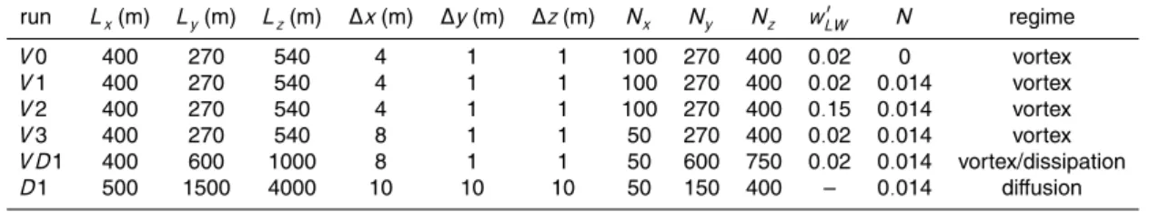
r2=(y2, z2), wherer=(y, z) denotes the vector position, and are separated byb0=47 m (see Fig. 1). The inital velocity field is given by

v0(y, z)=− Γ0 2π

z−z1

|r−r1|2



1−e

−|r−r1|2

2σ_c2



+

Γ0 2π

z−z2

|r−r2|2



1−e

−|r−r2|2

2σ_c2



 (10)

10

w0(y, z)=+ Γ0 2π

y −y₁

|r−r₁|2



1−e

−|r−r1|2

2σ2_c



−

Γ0 2π

y −y₂

|r−r₂|2



1−e

−|r−r2|2

2σ2_c



 (11)

whereσc=4.6 m is the core size andΓ0=600 m 2

s−1is the total circulation (these values are representative of a large-transport aircraft like a B747). In the three-dimensional simulations, the velocity field is copied in the axial direction and then perturbed to let the proper instability emerge. In particular, to mimic the effects of atmospheric turbulence 15

on the development of Crow instability, a simple perturbation of the vertical velocity is designed as (Robins and Delisi, 1998; Garten et al., 2001)

w₀′(x, y, z)=−w_LW′ VcB(y, z) cos

2πx λLW

(1+εrand) (12)

whereλLW ≃400 m is the Crow wavelength,B(x, y) is a step function equal to 1 inside

the vortex core and 0 outside, Vc=12.1 m s−1 is the maximum tangential velocity of

(11)

ACPD

9, 20429–20469, 2009

contrail-cirrus

Paugam et al.

Title Page

Tables Figures

◭ ◮

Back Close

Full Screen / Esc

Interactive Discussion the two vortices, whilew_LW′ is a parameter that sets the amplitude of the perturbation.

Gerz and Holz ¨apfel (1999) estimate the intensity of their three-dimensional anisotropic forcing field of about 3% to 1.7% of V_c over the horizontal and vertical respectively. The reference value was setw_LW′ =0.02 although other values were examinated up to w_LW′ =0.15 (see Table 1). The last term in Eq. (12) models the turbulence induced by 5

the jet via an additional white noise rand with an amplitude of 1% i.e.ε=0.01 (Holz äpfel et al., 2001). For all runs with ambient stratification, the Brunt-V äis äl ä frequency is N=1.4 10−2s−1a typical value at flight level of 11 km, (D ürbeck and Gerz, 1996) while the relative humidity is RH_i=130 %, which represents the most critical case from the environmental point of view as it allows the formation of contrail (RH_i>100%) without 10

natural cirrus (RH_i<140%).

Ice particles are initially radially distributed following a Gaussian law centered at the edge of vortex core, which is a reasonable approximation at the end of the jet phase as found for example by Paoli et al. (2004):

15

np(r)=nmax_i 

e

−|r−r1|2−σ2c σ_i2

+e

−|r−r2|2−σc2 σ2_i



 (13)

whereσ_i=σ_cwhilenmax_i is obtained from the identity

ZL_y

0

ZL_z

0

n_p(r)=Ni. (14)

The total number of ice particles per unit legnth of flight path N_i ≃ 1.5 1012m−1 and the initial particle radius r_i=1.5µm (assumed constant) are extrapolated from pre-20

(12)

ACPD

9, 20429–20469, 2009

contrail-cirrus

Paugam et al.

Title Page

Tables Figures

◭ ◮

Back Close

Full Screen / Esc

3 LES of contrail in the vortex regime

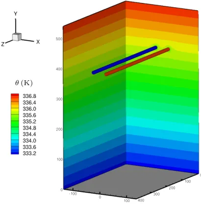
This section describes the main features that characterize the dynamics and the micro-physics of a contrail during the vortex regime (unless specified, the baseline configura-tion used for the analysis is runV1). As shown in the snapshots of velocity and vorticity fields in Fig. 2, the initial vortex pair (primary wake) descends in a density stratified en-5

vironment, detraining at the same time a curtain of material (secondary wake) that moves back to flight level. The origin of this secondary wake is the baroclinic torque generated at the edges of the primary wake that acts as a source of vorticity for the system:

Dω Dt=

1

ρ2∇ρ× ∇p. (15)

10

To leading order, the above equation reduces to the simpler form

Dωx

Dt =− gT

Π

∂(1/θ) ∂y =

g θ

∂θ

∂y (16)

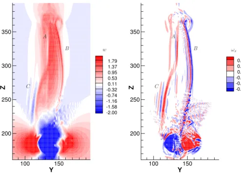
whereω_xis the axial vorticity andθis the potential temperature. The basic mechanism is represented in Fig. 3 that shows the evolution of the r.h.s. of Eq. (16): a negative (positive) torque is created at the right (left) edge of the primary wake, which are af-15

terwards advected toward the center of the wake where they form an upward-moving counter-rating vortex pair. Note that this is basically a two-dimensional mechanism that also occurrs in laminar wing wakes (Spalart, 1996).

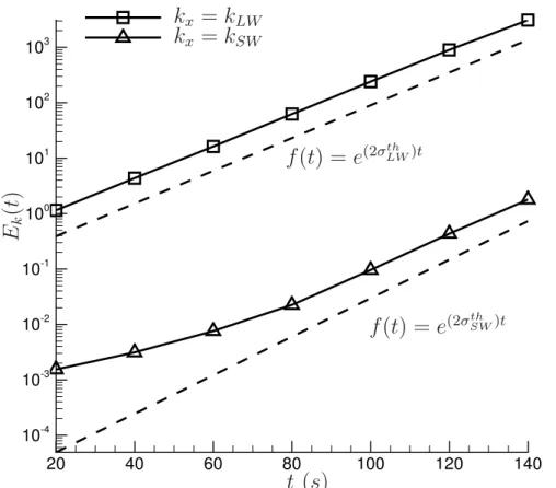
One of the main issue of the vortex regime is the combined action of the baroclinic torque, and theLW andSW three-dimensional instabilities that cause the break-up of 20

(13)

ACPD

9, 20429–20469, 2009

contrail-cirrus

Paugam et al.

Title Page

Tables Figures

◭ ◮

Back Close

Full Screen / Esc

Interactive Discussion In real stratified wakes, the baroclinic torque affects the development of the vortex

instabilities, represented in Fig. 5 by the isosurface of the λ2 invariant (Jeong and Hussain, 1995). Indeed, the growth rate of theSW instability depends on the vortex spacingb(Nomura et al., 2006):

σ_SW=σ_SWN0 b0

b (17)

5

so that when the vortices come closer by the action of the LW instability, b decreases and the SW instability grows faster. This in turns favors the break up of the vortices and enhances the decrease of the circulation and the final decay of the vortices (Holz ¨apfel et al., 2001; Laporte and Leweke, 2002; Holz ¨apfel et al., 2003).

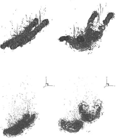
The e_ffect of the intensity of the initial perturbation is finally analyzed in Fig. 6 which 10

reports the isosurface of λ2 for two values wLW′ =0.02 and 0.15 (respectively run V1 and V2) at t=120 s and t=140 s. The interaction between the SW and LW instabili-ties is also a_ffected by the intensity of perturbation. In the case of high perturbation, the evolution of the Crow instability is clearly visible with the formation of vortex rings reconnecting after the break-up of the primary wake whereas in the low-perturbation 15

case, the dynamics is mainly controlled by the baroclinic torque and the SW instability. Indeed, the amplitude of the LW instability is too small to strongly affect the wake dy-namics and let the vortex rings form at the same wake age. This configuration might be commonly oberved in the sky, in fact the formation of puffs as described by Robins and Delisi (1998) does not occurr in all contrails. In what follows, we focus on the low 20

level turbulent case.

The turbulence generated by the vortex break-up and the consequent strong mixing with the atmosphere spread the wake mainly in the cross-direction. In order to treat the transition betweeen the vortex and the dissipation regimes until the wake-generated turbulence reaches the level of background atmospheric turbulence, the length of the 25

computational domain was increased to Ly=540 m and the resolution in the axial

(14)

ACPD

9, 20429–20469, 2009

contrail-cirrus

Paugam et al.

Title Page

Tables Figures

◭ ◮

Back Close

Full Screen / Esc

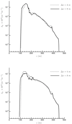
Interactive Discussion the distribution of scalar quanties, indeed Fig. 7 shows that the profiles of ice

num-ber density (which is a conserved scalar) are basically insensitive to the the axial grid resolution.

3.1 Microphysics in the vortex regime

In this section, the three-dimensional structure of the contrail is analyzed, the focus be-5

ing on the coupling between vortex dynamics and microphysics, and on the resulting non-homegeneity of microphysical properties such ice density and particle size distri-bution. Figure 8 shows the evolution of two isosurfaces of ice density colored with ice particle radius. The higher valueρi=10−5 kg/m3identifies the primary wake

contain-ing a large number of ice particles. These particles eventually evaporate at t=240 s 10

because of the adiabatic compression induced by the vortex descent; however, af-ter vortex break-up, a slight upwards displacement of the wake (induced by ambient stratification) creates an adiabatic expansion that again promotes and even amplifies condensation, as shown at the very bottom of the wake where large ice particles are formed att=320 s.

15

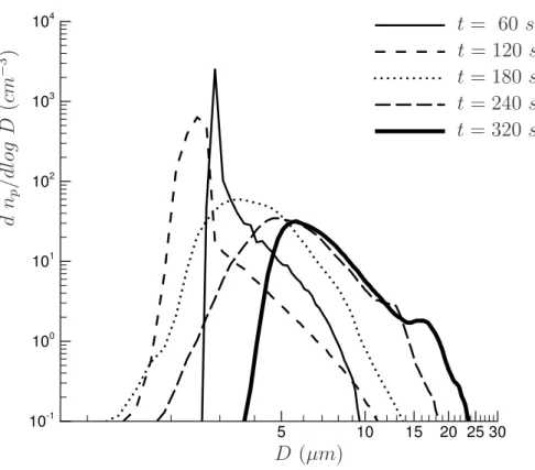
Figure 9 reports the evolution of ice particle size distribution for the reference simu-lationV D1 which shows a good agreement, in term of shape and order of magnitude, with the size distribution measured by Schr ¨oder et al. (2000). Indeed, in both cases the distribution first decreases and then shifts towards the large diameter which stands for the mixing with the supersaturated ambient atmosphere after the break-up of the 20

vortices.

Finally, Fig. 10 shows the optical depth τ of the contrail at the end of the vortex regime. This is estimated by

τ=

ZL_c

0

πr_i2Qext(ri)nid Lc (18)

whereL_c is the length of the contrail in the direction of observation while Qext is the 25

(15)

parti-ACPD

9, 20429–20469, 2009

contrail-cirrus

Paugam et al.

Title Page

Tables Figures

◭ ◮

Back Close

Full Screen / Esc

Interactive Discussion cles and was then taken constantQext=2 which is in the middle of the range 0<Qext<4

discussed by K ¨archer (1996). Figure 10 shows thatτ is consistent with satellite ob-servations (Sussmann and Gierens, 1999) whereτ∼1. However, unlike the results of Sussmann and Gierens (1999), only the primary wake is visible i.e. τ>0.03 accord-ing to K ¨archer (1996), which is likely due to the assumption made in the initial wake 5

perturbation in the vortex regime (i.e. a single Crow wavelegnth). The use of a three-dimnensional synthetic spectrum and, in general, the role of atmospheric turbulence in the development of Crow instability the will be investigated in a follow-up study).

4 The di_ffusion regime

This section covers the diffusion regime of the wake -and the most critical for contrail-10

to-cirrus transition, starting at approximatelyt=320 s after emission. At that time the potential temperature fluctuationsθ′∼0.1 K are of the same order of typical background fluctuations at the tropopause, so the interaction of the wake with the atmosphere -in particular the atmospheric turbulence- has to be taken into account.

To that end, a method has been developed to create a synthetic turbulent flow that 15

reproduces the statistics of velocity and temperature fluctuations at the tropopause (Schumann et al., 1995; D ¨urbeck and Gerz, 1996):

u′=v′=0.3 m s−1, w′=0.1 m s−1, θ′=0.1 K. (19)

Note that the physical processes that drive these fluctuations are not specified by the method. A comprehensive theory of the origin and the nature of turbulence at 20

tropopause is out of the scope of this paper as it represents a fundamental and still un-solved problem of atmospheric science since the first in situ measurements by Nastrom and Gage (1985) to the most recent work by Tulloch and Smith (2008).

(16)

ACPD

9, 20429–20469, 2009

contrail-cirrus

Paugam et al.

Title Page Abstract Introduction Conclusions References Tables Figures ◭ ◮ ◭ ◮ Back Close

Full Screen / Esc

Interactive Discussion flight level, the Richardson number is far greater than the limit needed to sustain

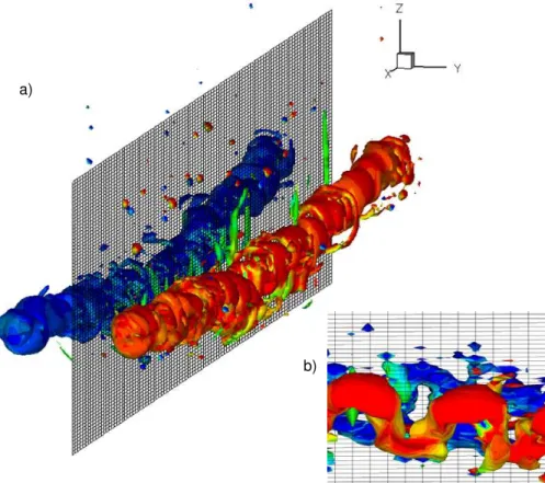
fluc-tuations as large as in Eq. (19) (i.e. Ri∼0.1). To generate atmospheric turbulence with proper characteristics we have used one of the functionalities of MesoNH to treat simul-taneously multiple models (running on the same computational domain in the present work): in the first model (“father”) an unstable stratified shear flow (Ri∼0.1) is used 5

to generate turbulent fluctuations of velocity and potential temperature: u′₁, v₁′, w₁′, θ₁′. These fluctuations are then used to force a second model (“son”) containing the con-trail (see Fig. 11). In practice this is done by adding suitable sources to the transport equations that drive the fluctuations in the second domain to the desired levels given by Eq. (19)

10

˙ uf=−

c_u t_f u−

u′_th u′₁ u1

!

(20)

˙ vf=−

c_v t_f v−

v_th′ v₁′ v1

!

(21)

˙

w_f=−cw

t_f w− w_th′

w₁′ w1

!

(22)

˙ θ_f=−cθ

t_f θ− θ′_th

θ₁′ θ1

!

(23)

where subscript 1 refers to quantities in the father domain,tf is an e-folding time which

15

is set equal to the time step, whilec_u, c_v, c_w, c_θ are scale factors for the forcing pa-rameters (see Paugam (2008) for technical details). The papa-rameters of the simulation in the diffusion regime (run D1) are summarized in Table 1. The computational do-main is 500 m,4000 m, 1500 m in the flight, cross, and vertical directions respectively and the resolution of 10 m in all directions. The turbulent flow generated by the shear 20

exhibits a well defined inertial range (Paugam, 2008), which allows one to identify an

eddy dissipation range; in a LES this can be deduced fromǫ=k 3/2

∆x=10 −4

(17)

ACPD

9, 20429–20469, 2009

contrail-cirrus

Paugam et al.

Title Page

Tables Figures

◭ ◮

Back Close

Full Screen / Esc

Interactive Discussion k ∼10−2m2s−2the subgrid-scale turbulent kinetic energy. The steady state values of

the turbulent fluctuations summarized in Table 2 are all in the range of typical values encountered at the tropopause (Sharman et al., 2005). Note that the ratio between the subgrid-scale and the total (resolved + subgrid-scale) turbulent kinetic energy is k/(k+K) ≃ 0.1<0.2 which satisfies the criterium of repartion of energy proposed by 5

Pope (2000) to asses the the quality of LES.

Furthermore, since the flow produced by the forcing is not isotropic in the flight direc-tion, the ice particle distribution at the end of the vortex/dissipation regime (runV D1) is averaged in this direction (see Fig. 11). This yields in the son model to an initial contrail withNi=1.54 1012m−1 particle per meter of flight, a mean ice particle radius

10

r_i=3.7µm, and aM_i=0.4 kg m−1ice mass per meter of flight. The ambient relative hu-midity is RH_i=130% whereas the stratification isN=0.014 s−1and no shear is applied.

4.1 Microphysics in the diffusion regime

Figure 12 reports the evolution of the horizontal σy and vertical σz spreading of the

contrail. These values are then used to identify the (turbulent) diffusion coefficients by 15

fitting a Gaussian plume:D_y=15 m2s andD_z ≃0, which are in fair agreement with the measurements by Schumann et al. (1995). Figure 13 shows the snapshots of super-saturation field over the 35 min of run D1. The ambient atmosphere is characterized by high humidity, whereas the contrail can be identified by the region withs_i∼0 where the excess of vapor has been condensed on ice particles. As indicated in Table 2 and 20

shown in the time evolution ofsi, the size of turbulent eddies isO(100 m) and is

main-tained throughout the whole simulation. Furthermore, the contrail spreads horizontally from 300 m to 1 km while it is confined in the vertical direction (i.e.Dz ≃0 m

2 s).

The evolution of ice number density and particle size distribution shown in Fig. 14 are consistent with the above picture that the spreading is almost horizontal during 25

(18)

ACPD

9, 20429–20469, 2009

contrail-cirrus

Paugam et al.

Title Page

Tables Figures

◭ ◮

Back Close

Full Screen / Esc

Interactive Discussion of atmospheric fluctuations (w′∼0.1 m s−1) so that sedimentation can affect the

verti-cal spreading as well. It is also interesting to observe that turbulent fluctuations lead to an homogeneization of the contrail-cirrus. In particular, Fig. 14 shows there is no real separation between the first and secondary wake, but the ice mostly grows at the edges of the contrail where the mixing with the ambient atmosphere is the strongest. 5

Att=35 min, a large number of small particles are still trapped inside the contrail. Af-terwards, these particles condense the ambient vapor and increase the overall ice content, as shown in Fig. 15.

Finally we analyze the evolution of the contrail optical depth, in particular, we are interested in finding out whether the number of ice particles nucleated in the very early 10

jet regime is high enough to explain the observed conservation of the optical depth in old contrails. This question, raised for the first time in the 90’s after the first in situ measurements (Jensen et al., 1998), is also relevant because it could give a strong ev-idence that no additional ice particles, other than those direclty formed on the exhaust particles, can be nucleated as the contrail evolve into a cirrus. The cross-sectional pro-15

files ofτ in Fig. 16 confirm this picture, in fair agreement with results of Jensen et al. (1998) who used a sophisticated model including sedimentation and radiative heating. On the other hand, our results rather suggest that atmospheric turbulence is one of the driving mechanisms that lead to the conservation ofτ∼n r2 up to 30 min. Indeed, in spite of the drop of particle number density by diffusion (see Fig. 16), tubulent fluctua-20

tions promote the growth of the average ice surface (∼r2) in such a way that the peak ofτremains almosy constant (see Eq. 18). It is also interesting to note that the order of magnitude ofτin the present simulations is in the range of satellite measurements (At-las et al., 2006) which give a maximum and a mean value ofτmax∼1.4 andτmean∼0.3, respectively. This also validates a posteriori the choice on the condensational model 25

(19)

ACPD

9, 20429–20469, 2009

contrail-cirrus

Paugam et al.

Title Page

Tables Figures

◭ ◮

Back Close

Full Screen / Esc

5 Conclusions and perspectives

In this work, the evolution of a contrail and its transition into a contrail-cirrus was studied by means of high-resolution numerical simulations. The main features of vortex dynam-ics in stratified flows, such as the vortex instability and the baroclinic torque, were well captured by the model and their interaction with ice microphyscis was discussed. In the 5

late diffusion regime the transition between contrail and cirrus was reproduced by forc-ing a synthetic sheared turbulence that mimics real anisotropic atmospheric turbulence. The contrail-cirrus was found to spread out mostly in the horizontal direction, whereas its contrail optical depth was conserved despite its diffusion, in good agreement with observations.

10

Besides showing the feasibility of three-dimensional contrail simulations, the results of this study also serve as starting point to go beyond the 35 min simulation, so as to provide the raw data -on time scales of one to two hours- that are needed to param-eterize the contrail-cirrus into global climate models. To that end, the present model is being further developed to include the radiative forcing associated to the ice crys-15

tal distribution and to account for various meteorological conditions. In addition to the relative humidity of background air and the influence of ice distribution at the begin-ning of the diffusion regime, vertical wind shear and possible large-scale uplift of the atmosphere due to synoptic structures and its associated adiabatic cooling will be con-sidered. Finally, the extension to full coupling between three-dimensional dynamics, 20

microphysics and the chemical processes including homogeneous and heterogeneous chemistry, and its application to the parameterization of aircraft contrail-cirrus in Global Circulation Models is another important topic that will also be addressed in the future.

Acknowledgements. This work was supported by the European Union FP6 Integrated Project QUANTIFY (http://www.pa.op.dlr.de/quantify/), the French LEFE/CHAT INSU programme (http:

25

(20)

ACPD

9, 20429–20469, 2009

contrail-cirrus

Paugam et al.

Title Page

Tables Figures

◭ ◮

Back Close

Full Screen / Esc

The publication of this article is financed by CNRS-INSU.

References

Atlas, D., Wang, Z., and Dupa, D. P.: Contrails to Cirrus - Morphology, Microphysics and Radia-tive Properties, J. Appl. Meteorol. Climatol., 45, 5–19, 2006. 20446

5

Chlond, A.: Large Eddy simulation of Contrails, J. Atmos. Sci., 55, 796–819, 1996. 20433 Crow, S. C.: Stability Theory for a Pair of Trailing Vortices, AIAA J., 8, 2172–2179, 1970. 20431 Cuxart, J., Bougeault, P., and Redelsperger, J.-L.: A turbulence scheme allowing for mesoscale

and large scale eddy simulations, Q. J. Roy. Meteorol. Soc., 126, 1–30, 2000. 20434 Darracq, D., Corjon, A., Ducros, F., Keane, M., Buckton, D., and Redfern, M.: Simulation of

10

wake vortex detection with airborne Doppler lidar, J. Aircr., 37, 984–993, 2000. 20434 D ¨ornbrack, A. and D ¨urbeck, T.: Turbulent Dispersion of Aircraft Exhausts in Regions of Breaking

Gravity Wave, Atmos. Environ., 32, 3105–3112, 1998. 20432

D ¨urbeck, T. and Gerz, T.: Dispersion of aircraft exhausts in the free atmosphere, J. Geophys. Res., 101, 26007–26016, 1996. 20432, 20439, 20443

15

Garten, J. F., Arendt, S., Fritts, D. C., and Werne, J.: Dynamics of counter-rotating vortex pairs in stratified and sheared environments, J. Fluid Mech., 361, 189–236, 1998. 20438

Garten, J. F., Werne, J., Fritts, D. C., and Arendt, S.: Direct numerical simulation of the Crow instability and subsequent vortex reconnection in a stratified fluid, J. Fluid Mech., 426, 1–45, 2001. 20438

20

Gerz, T. and Holz ¨apfel, F.: Wing-Tip Vortices, Turbulence and the Distribution of Emissions, AIAA J., 37, 1270–1276, 1999. 20432, 20433, 20434, 20437, 20439

(21)

ACPD

9, 20429–20469, 2009

contrail-cirrus

Paugam et al.

Title Page

Tables Figures

◭ ◮

Back Close

Full Screen / Esc

Gierens, K. and Jensen, E.: A numerical study of the contrail-to-cirrus transition, Geosphys. Res. Lett., 25, 4341–4344, 1998. 20432, 20433, 20437

Gierens, K., Schumann, U., Helten, M., Smit, H., and Marenco, A.: A distribution law for rel-ative humidity in the upper troposphere and lower stratosphere derived from three years of MOZAIC measurements, Ann. Geophys., 17, 1218–1226, 1999,

5

http://www.ann-geophys.net/17/1218/1999/. 20434

Heymsfield, A. J. and Iaquinta, J.: Cirrus Crustal Terminal Velocities, J. Atmos Sci., 57, 916– 938, 1999. 20436

Holz ¨apfel, F., Gerz, T., and Baumann, R.: The turbulent decay of trailing vortex pairs in stably stratified environments, Aerosp. Sci. Technol., 5, 95–108, 2001. 20432, 20437, 20439, 20441

10

Holz ¨apfel, F., Hofbauer, T., Darracq, D., Moet, H., Garnier, F., and Ferreira Gago, C.: Analysis of wake vortex decay mechanisms in the atmosphere, Aerosp. Sci. Technol., 7, 263–275, 2003. 20441

Jacquin, L. and Garnier, F.: On the dynamics of engine jets behind a transport aircraft, AGARD CP-584, NATO, 1996. 20438

15

Jensen, E., Ackerman, A. S., Stevens, D. E., B.Tonn, O., and Minnis, P.: Spreding and growth of contrails in a sheared environment, J. Geophys. Res., 103, 31557–31567, 1998. 20432, 20433, 20446

Jeong, J. and Hussain, F.: On the identification of a vortex, J. Fluid Mech., 285, 69–94, 1995. 20441, 20458

20

Kaltenback, H.-J., Gerz, T., and Schumann, U.: Large-eddy simulation of homogeneus turbu-lence abd diffusion in stably stratified shear flow, J. Fluid Mech., 280, 1–40, 1994. 20433, 20443

K ¨archer, B.: The initial composition of the jet condensation trails, J. Atmos. Sci., 73, 3066–3082, 1996. 20435, 20443

25

K ¨archer, B.: Physicochemistry of aircraft-generated liquid aerosols, soot, and ice particles 1. Model description, J. Geophys. Res., 103, 17111–17128, 1998. 20435

Lafore, J. P., Stein, J., Asencio, N., Bougeault, P., Ducrocq, V., Duron, J., Fischer, C., H ´ereil, P., Mascart, P., Masson, V., Pinty, J. P., Redelsperger, J. L., Richard, E., and Vil ´a-Guerau de Arellano, J.: The Meso-NH Atmospheric Simulation System. Part I: adiabatic formulation

30

and control simulations, Ann. Geophys., 16, 90–109, 1998, http://www.ann-geophys.net/16/90/1998/. 20434

(22)

ACPD

9, 20429–20469, 2009

contrail-cirrus

Paugam et al.

Title Page

Tables Figures

◭ ◮

Back Close

Full Screen / Esc

Direct NumericalSimulation, AIAA J., 40, 2483–2494, 2002. 20441

Lewellen, D. C. and Lewellen, W. S.: The Effects of Aircraft Wake Dynamics on Contrail Devel-opment, J. Atmos. Sci., 58, 390–406, 2001. 20432, 20436, 20437

Lynch, D., Sassen, K., Starr, D. O., and Stephens, G.: Cirrus, Oxford University Press, 2002. 20439

5

Mannstein, H. and Schumann, U.: Aircraft induced contrail cirrus over Europe, Meteor. Z., 14, 549–554, 2005. 20432

Meyer, R., Mannstein, H., Meerk ¨otter, R., Schumann, U., and Wendling, P.: Regional radiative forcing by line-shaped contrails derived from satellite data, J. Geophys. Res., 107, p. 4104, 2002. 20432

10

Minnis, P., Young, D. F., and Garber, D. P.: Transformation of contrails into cirrus during SUC-CESS, Geophys. Res. Lett., 25, 1157–1160, 1998. 20432

Nastrom, G. D. and Gage, K. S.: A climatology of atmospheric wave number spectra of wind and temperature observed by commercial aircraft, J. Atmos. Sci., 42, 950–960, 1985. 20443 Nomura, K. K., Tsutsui, H., Mahoney, D., and Rottman, J. W.: Short-wavelength instability and

15

decay of a vortex pair in a stratified fluid, J. Fluid Mech., 553, 283–322, 2006. 20441 Paoli, R., H ´elie, J., and Poinsot, T.: Contrails formation in aircraft wakes, J. Fluid Mech., 502,

361–373, 2004. 20432, 20437, 20439

Paugam, R.: Simulation num érique de l’ évolution d’une traˆın ée de condensation et de son in-teraction avec la turbulence atmosph érique, Ph.D. thesis, Ecole Centrale Paris, 2008. 20437,

20

20439, 20440, 20444

Penner, J. E., Lister, D. H., Griggs, D. J., Dokken, D. J., and McFarland, M.: Aviation and the Global Atmosphere, Tech. rep., Intergovernmental Panel on Climate Change, 1999. 20430 Ponater, M., Brinkop, S., Sausen, R., and Schumann, U.: Simulating the global atmospheric

response to aircraft water vapour emissions and contrails: a first approach using a GCM,

25

Ann. Geophys., 14, 941–960, 1996,

http://www.ann-geophys.net/14/941/1996/. 20431

Pope, S. B.: Ten questions concerning the large-eddy simulation of turbulent flows, New J. Phys., 6(35), 2004. 20445

Robins, R. E. and Delisi, D. P.: Numerical Simulation of Three-Dimensional Trailing Vortex

30

Evolution in Stratified Fluid, AIAA J., 36, 981–985, 1998. 20438, 20441

(23)

ACPD

9, 20429–20469, 2009

contrail-cirrus

Paugam et al.

Title Page

Tables Figures

◭ ◮

Back Close

Full Screen / Esc

IPCC, Meteorol. Z., 14, 555–561, 2005. 20430, 20431

Schr öder, F., K ärcher, B., Duroure, C., Str öm, J., Petzold, A., Gayet, J.-F., Strauss, B., Wendling, P., and Borrmann, S.: On the transition of Contrails into Cirrus Clouds, J. Atmos. Sci., 57, 464–480, 2000. 20432, 20442

Schumann, U.: On conditions for contrail formation from aircraft exhausts, Meteorol. Z., 5,

5

4–23, 1996. 20432

Schumann, U.: Formation, properties and climatic effects of contrails, Comptes Rendus Physique, 6, 549–565, 2005. 20430

Schumann, U., Konopka, P., Baumann, R., Busen, R., Gerz, T., Schlager, H., Schulte, P., and Volkert, H.: Estimate of diffusion parameters of aircraft exhaust plumes near the tropopause

10

from nitric oxide and turbulence measurements, J. Geophys. Res., 100, 14147–14162, 1995. 20433, 20443, 20445, 20465

Sharman, R., Tebaldi, C., Wiener, G., and Wol_ff, J.: An Integrated Approcah to Mid- and Upper-Level Turbulence Forecasting, Weather Forcast., 21, 268–286, 2005. 20445

Sonntag, D.: Advencements in the field of hygrometry, Meteorol. Z., 3, 51–56, 1994. 20436

15

Spalart, P. R.: On the motion of laminar wing wakes in a stratified fluid, J. Fluid Mech., 327, 139–160, 1996. 20440

Spalart, P. R.: Airplane trailing vortices, Annu. Rev. Fluid Mech., 30, 107–148, 1998. 20438 Sussmann, R. and Gierens, K.: Lidar and numerical studies on the different evolution of

vor-tex pair and secondary wake in young contrails, J. Geophys. Res., 104, 2131–2142, 1999.

20

20431, 20432, 20433, 20434, 20443

Travis, D. J., Carleton, A. M., and Lauritsen, R. G.: Jet Contrails and Climate: Anomalous In-creases in U.S. Diurnal Temperature Range for September 11-14, 2001, Nature, 418, p. 601, 2002. 20431

Tulloch, R. and Smith, K. S.: A baroclinic model for the atmospheric energy spectrum, J. Atmos.

25

Sci., 66, 450–467, 2008. 20443

(24)

ACPD

9, 20429–20469, 2009

contrail-cirrus

Paugam et al.

Title Page

Tables Figures

◭ ◮

Back Close

Full Screen / Esc

Table 1.List of parameters of the numerical simulations.

run Lx(m) Ly(m) Lz(m) ∆x(m) ∆y(m) ∆z(m) Nx Ny Nz wLW′ N regime

V0 400 270 540 4 1 1 100 270 400 0.02 0 vortex

V1 400 270 540 4 1 1 100 270 400 0.02 0.014 vortex

V2 400 270 540 4 1 1 100 270 400 0.15 0.014 vortex

V3 400 270 540 8 1 1 50 270 400 0.02 0.014 vortex

V D1 400 600 1000 8 1 1 50 600 750 0.02 0.014 vortex/dissipation

(25)

ACPD

9, 20429–20469, 2009

contrail-cirrus

Paugam et al.

Title Page

Tables Figures

◭ ◮

Back Close

Full Screen / Esc

Table 2. Parameters of the synthetic turbulence generated in the diffusion regime: v′, w′, horizontal and vertical velocity fluctuations;θ′, potential temperature fluctuations;k, turbulent kinetic energy; ǫ, eddy dissipation rate; k/(k +K), ratio between the resolved and the total kinetic energy;L_v,L_w, size of horizontal and vertical eddies.

(26)

ACPD

9, 20429–20469, 2009

contrail-cirrus

Paugam et al.

Title Page

Tables Figures

◭ ◮

Back Close

Full Screen / Esc

θ(K)

Fig. 1. Initial vortex field and background potential temperature. The red (blue) isosurfaces

(27)

ACPD

9, 20429–20469, 2009

contrail-cirrus

Paugam et al.

Title Page

Tables Figures

◭ ◮

Back Close

Full Screen / Esc

Y

Z

100 150

200 250 300 350

1.79 1.37 0.95 0.53 0.11 -0.32 -0.74 -1.16 -1.58 -2.00 w A

B

C

Y

Z

100 150

200 250 300 350

0.5 0.3 0.1 -0.1 -0.3 -0.5 ω_x A

B

C

(28)

ACPD

9, 20429–20469, 2009

contrail-cirrus

Paugam et al.

Title Page

Tables Figures

◭ ◮

Back Close

Full Screen / Esc

∂(1/θ)

∂y ×10

−6

(K−1

)

Fig. 3. Generation of the secondary wake in the cross-section yz at x=200 m (axial

loca-tion of minimal vortex spacing): Isocontours of the source of axial vorticity: ∂_∂y1/θ see Eq. (16) and isolines of axial vorticity (4 levels between −0.5 s−1 and 0.5 s−1). From left to right:

(29)

ACPD

9, 20429–20469, 2009

contrail-cirrus

Paugam et al.

Title Page

Tables Figures

◭ ◮

Back Close

Full Screen / Esc

20 40 60 80 100 120 140

10-4 10-3 10-2 10-1 100 101 102 103

t

(

s

)

E

k

(

t

)

k

x

=

k

LW

k

x

=

k

SW

f

(

t

) =

e

(2σLWth )t

f

(

t

) =

e

(2σthSW)t

(30)

ACPD

9, 20429–20469, 2009

contrail-cirrus

Paugam et al.

Title Page

Tables Figures

◭ ◮

Back Close

Full Screen / Esc

a)

b)

(31)

ACPD

9, 20429–20469, 2009

contrail-cirrus

Paugam et al.

Title Page

Tables Figures

◭ ◮

Back Close

Full Screen / Esc

Fig. 6. Effects of initial perturbation on the isosurface λ₂=−0.3 of the vorticity invariant at

(32)

ACPD

9, 20429–20469, 2009

contrail-cirrus

Paugam et al.

Title Page

Tables Figures

◭ ◮

Back Close

Full Screen / Esc

0 100 200 300 400 500 10-9

10-7 10-5 10-3 10-1

z(m)

˜

np

×

10

1

1(

m

−

1m

−

1)

∆x= 4m

∆x= 8m

0 100 200 300 400 500 10-9

10-7 10-5 10-3 10-1

z(m)

˜

np

×

10

1

1(

m

−

1m

−

1)

∆x= 4m

∆x= 8m

(33)

ACPD

9, 20429–20469, 2009

contrail-cirrus

Paugam et al.

Title Page

Tables Figures

◭ ◮

Back Close

Full Screen / Esc

ri

Fig. 8. Three-dimensional structure of the contrail during the vortex regime and dissipation

regimes (runV D1): evolution of ice density isosurfacesρ_i=2 10−6 (left) andρ_i=10−5kg m−3 (right) colored with isocontours of ice particle radiusr_i. The isolines of the vorticty invariant

(34)

ACPD

9, 20429–20469, 2009

contrail-cirrus

Paugam et al.

Title Page

Tables Figures

◭ ◮

Back Close

Full Screen / Esc

5 10 15 20 25 30

10-1

100

101

102

103

104

D

(

µm

)

d

n

p

/d

lo

g

D

(

cm

−

3

)

t

= 60

s

t

= 120

s

t

= 180

s

t

= 240

s

t

= 320

s

(35)

ACPD

9, 20429–20469, 2009

contrail-cirrus

Paugam et al.

Title Page

Tables Figures

◭ ◮

Back Close

Full Screen / Esc

τ

Fig. 10.Two-dimensional distributions of the optical depthτin thexzplane (left panel) andxy

(36)

ACPD

9, 20429–20469, 2009

contrail-cirrus

Paugam et al.

Title Page

Tables Figures

◭ ◮

Back Close

Full Screen / Esc

d

dzu

u′_{, v}′_{, w}′_{, θ}′

x

x y

y z

z

(37)

ACPD

9, 20429–20469, 2009

contrail-cirrus

Paugam et al.

Title Page

Tables Figures

◭ ◮

Back Close

Full Screen / Esc

500 1000 1500 2000

0 1 2 3 4

t

(

s

)

σ

2

,

_y

σ

2 _z

×

10

4

(

m

2

)

σ

y

σ

z

σ

2y− p

=

2 D

h

t,

D

y

=

15 m

2

s

−

1

(38)

ACPD

9, 20429–20469, 2009

contrail-cirrus

Paugam et al.

Title Page

Tables Figures

◭ ◮

Back Close

Full Screen / Esc

si

(39)

ACPD

9, 20429–20469, 2009

contrail-cirrus

Paugam et al.

Title Page

Tables Figures

◭ ◮

Back Close

Full Screen / Esc

ni

ri

(40)

ACPD

9, 20429–20469, 2009

contrail-cirrus

Paugam et al.

Title Page

Tables Figures

◭ ◮

Back Close

Full Screen / Esc

102 103

10-2 10-1 100

t

(

s

)

M

m

V

o

l

g

(

k

g

m

−

1

)

(41)

ACPD

9, 20429–20469, 2009

contrail-cirrus

Paugam et al.

Title Page

Tables Figures

◭ ◮

Back Close

Full Screen / Esc

1500 2000 2500

0 2 4 6 8 10

y(m)

ni

y

(

×

1

.

10

9m

−

1)

t= 320s t= 2120s

1400 1600 1800 2000 2200 2400 2600

0 0.2 0.4 0.6 0.8 1

y(m)

τ

t= 320s t= 2120s

Fig. 16. Spanwise distributions of ice particle number density n_i

y (left) and optical depth τ

(right) integrated in thexzdirection, showing the conservation ofτduring the diffusion regime despite the decrease ofn_i