QUAGMIRE v1.3: a quasi-geostrophic model for investigating rotating fluids experiments

(1)

GMDD

1, 187–241, 2008

QUAGMIRE v1.3

P. D. Williams et al.

Title Page

Abstract Introduction

Conclusions References

Tables Figures

◭ ◮

Back Close

Full Screen / Esc

Printer-friendly Version

Interactive Discussion Geosci. Model Dev. Discuss., 1, 187–241, 2008

www.geosci-model-dev-discuss.net/1/187/2008/ © Author(s) 2008. This work is distributed under the Creative Commons Attribution 3.0 License.

Geoscientific Model Development Discussions

Geoscientific Model Development Discussionsis the access reviewed discussion forum ofGeoscientific Model Development

QUAGMIRE v1.3: a quasi-geostrophic

model for investigating rotating fluids

experiments

P. D. Williams1, T. W. N. Haine2, P. L. Read3, S. R. Lewis4, and Y. H. Yamazaki3

1

National Centre for Atmospheric Science, Department of Meteorology, University of Reading, Reading, UK

2

Department of Earth and Planetary Sciences, Johns Hopkins University, MD, USA

3

Atmospheric, Oceanic and Planetary Physics, Department of Physics, University of Oxford, Oxford, UK

4

Department of Physics and Astronomy, Open University, Milton Keynes, UK

Received: 8 August 2008 – Accepted: 17 August 2008 – Published: 5 September 2008

Correspondence to: P. D. Williams ([email protected])

(2)

GMDD

1, 187–241, 2008

QUAGMIRE v1.3

Title Page

Tables Figures

◭ ◮

Back Close

Full Screen / Esc

Interactive Discussion

Abstract

QUAGMIRE is a quasi-geostrophic numerical model for performing fast, high-resolution simulations of multi-layer rotating annulus laboratory experiments on a desktop per-sonal computer. The model uses a hybrid finite-difference/spectral approach to numer-ically integrate the coupled nonlinear partial differential equations of motion in

cylindri-5

cal geometry in each layer. Version 1.3 implements the special case of two fluid layers of equal resting depths. The flow is forced either by a differentially rotating lid, or by relaxation to specified streamfunction or potential vorticity fields, or both. Dissipation is achieved through Ekman layer pumping and suction at the horizontal boundaries, including the internal interface. The effects of weak interfacial tension are included,

10

as well as the linear topographic beta-effect and the quadratic centripetal beta-effect. Stochastic forcing may optionally be activated, to represent approximately the effects of random unresolved features. A leapfrog time stepping scheme is used, with a Robert filter. Flows simulated by the model agree well with those observed in the correspond-ing laboratory experiments.

15

1 Introduction

For over a century, geoscientists have invoked the principles of dynamical similarity (e.g. Douglas and Gasiorek, 2000) and geometrical similarity in order to study plane-tary atmospheres and oceans indirectly in the laboratory. For example, the mid-latitude atmospheric flow on a rotating planet closely resembles the flow in a rotating laboratory

20

annulus, as suggested by Fig. 1. This statement holds despite typical length and time scales for corresponding atmospheric and laboratory phenomena differing by many or-ders of magnitude. What matters is equality of the relevant non-dimensional parame-ters, such as the Rossby number (for dynamical similarity) and the horizontal-to-vertical aspect ratio (for geometrical similarity).

25

Once a particular fluid flow problem has been solved by making observations in the

(3)

GMDD

1, 187–241, 2008

QUAGMIRE v1.3

Title Page

Tables Figures

◭ ◮

Back Close

Full Screen / Esc

Interactive Discussion laboratory, an infinite number of other fluid flow problems have also effectively been

solved, all of which are dynamically and geometrically similar. The main benefits of laboratory experiments are that they are under the complete control of the operator; that global high-resolution measurements may be taken; and that controlled experi-ments may be repeated as many times as required. None of these stateexperi-ments holds

5

when the atmosphere and oceans are studied directly.

A review of the role of laboratory experiments in geophysical fluid dynamics has been given by Hide (1977). Laboratory investigations of non-rotating fluids began in the nineteenth century, and include the classic experiments of Reynolds (1883). At around the same time, Vettin (1884) was probably the first to exploit dynamical similarity by

10

carrying out rotating laboratory experiments as analogues of geophysical flows. He studied the surface flow in a rotating dishpan of fluid with a lump of ice near the centre, representing a polar ice cap, and he drew meteorological conclusions from his results (to the scorn of his contemporaries).

For the most direct resemblance between annulus and planet, heating and cooling

15

should be applied at the outer and inner sidewalls, respectively, in order to mimic the equator-to-pole temperature gradient. However, it follows from thermal (and gradient) wind balance that a radial temperature gradient will be accompanied by a vertical shear in the zonal velocity. Therefore, analogous flows may be obtained in an isothermal an-nulus by directly imposing a shear using a differentially-rotating lid. The

continuously-20

stratified thermally-forced rotating annulus and the two-layer mechanically-forced rotat-ing annulus have both been studied extensively (e.g. Hide et al., 1977; Carrigan, 1978; King, 1979; Appleby, 1982; Lovegrove, 1997; Williams, 2003).

The development of computer models for simulating the general circulation of plane-tary atmospheres and oceans has been accompanied by the development of computer

25

(4)

pa-GMDD

1, 187–241, 2008

QUAGMIRE v1.3

Title Page

Tables Figures

◭ ◮

Back Close

Full Screen / Esc

Interactive Discussion per, we describe the development of a numerical model for simulating fluid flows in the

multi-layer rotating annulus. The model is named QUAGMIRE, theQUAsi-Geostrophic Model for Investigating Rotating fluids Experiments.

Section 2 reviews a variety of possible modelling approaches, each making different dynamical and geometrical assumptions. A balanced model with a full representation

5

of the cylindrical geometry is the preferred approach, for a number of important rea-sons which are discussed. The two-layer quasi-geostrophic coupled partial differential equations in cylindrical coordinates are derived in Sect. 3, and the diagnostic relations between streamfunction and potential vorticity are decomposed into vertical and az-imuthal normal mode form in order to simplify their solution. Suitable sidewall boundary

10

conditions are derived by considering integral properties of the governing equations. Then, the continuous equations are carefully discretized in Sect. 4, in such a way as to preserve discrete analogues of the integral properties. Suitable initial conditions and numerical parameter values are given. In Sect. 5, the calculations are partitioned into model subroutines, and the technical details of how to run the model are described.

15

The code is tested in order to ensure that it is free from errors. The paper concludes with a summary in Sect. 6.

2 Models of the rotating annulus

In this section, the relative merits of different possible dynamical (Sect. 2.1) and geo-metrical (Sect. 2.2) choices will be summarised.

20

2.1 Possible dynamical choices

For numerically modelling the laboratory annulus, one possible approach would be a direct numerical simulation (DNS) of the Navier-Stokes equations or shallow-water equations, which are both referred to as primitive equations because only minor ap-proximations are made and both vortical and divergent eigenmodes are retained. DNS

25

(5)

GMDD

1, 187–241, 2008

QUAGMIRE v1.3

Title Page

Tables Figures

◭ ◮

Back Close

Full Screen / Esc

Interactive Discussion codes have been developed for the continuously-stratified thermally-forced rotating

an-nulus (e.g. Hignett et al., 1985; White, 1986) but they are computationally expensive and generally can be used to examine a small number of case-study flows only.

As an alternative to the existing DNS models, in this paper we develop a balanced model in which the divergent eigenmodes are filtered out by construction. The

filter-5

ing is justified because the interaction between vortical and divergent eigenmodes is thought to be weak. Balanced models have fewer dynamical degrees of freedom than primitive equation models, and therefore run much more quickly, allowing larger num-bers of simulations to be performed.

Three possible balanced models for multi-layer flows are those based on the quasi-10

geostrophic equations, the balance equations and the slow equations. These three equation sets are each derived from the shallow-water equations, which in turn are de-rived from the Navier-Stokes equations by assuming hydrostatic balance and columnar flow. Discussions of these and other filtered models are given by McWilliams and Gent (1980) and McIntyre and Norton (2000).

15

The quasi-geostrophic equations (Charney et al., 1950) are derived by assuming that the potential vorticity is advected only by the geostrophic component of the flow, and that interface perturbations are much smaller than the mean layer depths.

The balance equations (Charney, 1955) are derived by performing a horizontal ve-locity decomposition into vortical and divergent components, and then truncating with

20

respect to the divergent component. The balance described is more complicated, but also more accurate, than geostrophic balance. Efficient procedures have been de-veloped for integrating the balance equations (Daley, 1982). However, in their most general form the balance equations have spurious non-physical wave solutions with phase speeds much larger than those of inertia-gravity waves (Moura, 1976).

25

(6)

GMDD

1, 187–241, 2008

QUAGMIRE v1.3

Title Page

Tables Figures

◭ ◮

Back Close

Full Screen / Esc

Interactive Discussion the shallow-water equations.

Of the above three possible dynamical choices, the quasi-geostrophic (Q-G) equa-tions are used for the QUAGMIRE model developed in this paper. This is because only one scalar function of horizontal position per layer (the streamfunction) is needed to uniquely define the state of the system in a Q-G model, whereas three per layer (the

5

streamfunction, velocity potential and geopotential) are needed in a balance equations or slow equations model. With three times fewer dependent variables, the computa-tional advantages gained from using a Q-G model arguably outweigh the disadvan-tages of its slightly lower formal accuracy.

2.2 Possible geometrical choices

10

Brugge et al. (1987) have developed a numerical Q-G model for simulating multi-layer flows in a rectangular channel. However, their model is not particularly suitable for simulating the flow in the laboratory annulus, for the following reasons.

First, the channel equations with periodic azimuthal boundary conditions are a good approximation to the annulus equations only if the width of the annular gap is much

15

smaller than the mean radius (King, 1979). With this condition satisfied, the curvature becomes negligible and it would be possible to justify the use of a channel model to simulate the flow in an annulus. For typical laboratory annulus experiments, however, the condition is not satisfied.

Second, channel models have additional shift-reflect symmetries not present in

an-20

nulus models (Cattaneo and Hart, 1990). This is because, although the annulus and periodic channel are topologically similar, the geometry of their boundaries is funda-mentally different. For example, there is a reflect symmetry in the channel in the plane which is equidistant from the sidewalls, but there is no analogous symmetry in the annulus. Kwon and Mak (1988) show that the existence of such additional

symme-25

tries in the periodic channel leads to certain vortical wave-wave interaction coefficients being identically zero. Only models in cylindrical geometry admit the complete set of wave-wave interactions.

(7)

GMDD

1, 187–241, 2008

QUAGMIRE v1.3

Title Page

Tables Figures

◭ ◮

Back Close

Full Screen / Esc

Interactive Discussion Third, the channel and the annulus both contain background potential vorticity

gradi-ents, due to the sloping of equilibrium geopotential height surfaces in the presence of a vertical shear in horizontal velocity. In the channel, these geopotential height and po-tential vorticity variations are linear in the across-channel direction, but in the annulus they are quadratic because of the parabolic equilibrium interface height shape

pro-5

duced by centripetal effects. This is known as thequadratic β-effect and is captured only by using cylindrical geometry.

Finally, the model of Brugge et al. (1987) does not include the effects of interfacial tension, which can be significant in the laboratory.

For the above reasons, the existing multi-layer Q-G models are not particularly

suit-10

able for simulating the flow in the laboratory annulus. Therefore, the remainder of this paper describes the construction of a new model which takes into account cylindrical geometry and interfacial tension.

3 Continuous equations

In this section, the governing continuous equations are derived (Sect. 3.1) and

decom-15

posed into normal mode form (Sect. 3.2), and suitable boundary conditions are derived (Sect. 3.3).

3.1 Derivation from first principles

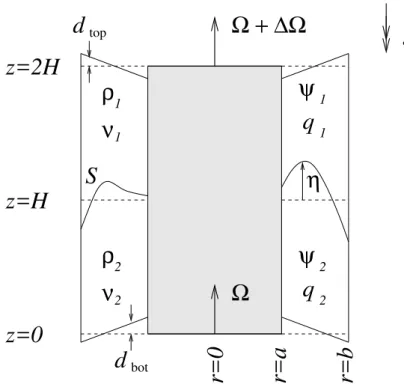
The annulus to be modelled is shown schematically in Fig. 2. We use cylindrical po-lar coordinates, r=(r, θ, z). The z-axis is coincident with the rotation axis. The fluid 20

is bounded by a base of mean vertical position z=0, a lid of mean vertical position z=2H>0 and cylindrical walls at r=a and r=b>a. The base and lid linearly devi-ate from their mean vertical positions bydbot(r) and dtop(r). We define the constants

sbot=ddbot/dr andstop=ddtop/dr. The two homogeneous, immiscible layers have

(8)

GMDD

1, 187–241, 2008

QUAGMIRE v1.3

Title Page

Tables Figures

◭ ◮

Back Close

Full Screen / Esc

Interactive Discussion the oceanographic convention thati=1 refers to the upper layer andi=2 to the lower

layer. The undisturbed fluid interface is atz=H and the disturbed fluid interface is at z=H +η(r, t). The acceleration due to gravity is g. The base and sidewalls rotate

about the axis of symmetry with angular velocityΩ, and the lid rotates about the axis of symmetry with angular velocityΩ + ∆Ω.

5

In the frame which rotates with the base, the four fundamental equations for the pressure,p_i(r, t), and the velocity,u_i(r, t), are the Navier-Stokes equations,

∂u_i

∂t +(ui ·∇)ui+2Ω×ui +Ω×(Ω×r)=− 1

ρ_i∇pi +νi∇

2

u_i +g, (1)

and the equation of volume conservation for the incompressible liquids,

∇·u_i =0. (2)

10

Defining the vorticity byω_i=∇×u_i, we take the curl of Eq. (1) and use vector identities

to obtain ∂ω_i

∂t +(ui·∇)ωi =[(2Ω+ωi)·∇]ui +νi∇

2

ω_i , (3)

the z-component of which, in the fluid interiors (i.e. away from the boundary layers) where the flow is assumed to be columnar and inviscid, is

15

∂ξ_i

∂t +(ui·∇)ξi =(f +ξi) ∂ui , z

∂z , (4)

where ξ_i is the z-component of ω_i, f=2Ω is the Coriolis parameter and u_{i , z} is the

vertical velocity.

We next vertically integrate Eq. (4) over the fluid interiors, parameterizing vertical Ekman pumping and suction velocities (Gill, 1982) at the lid, base and interface, which

20

are all assumed to have small slopes. Assuming that the Ekman layer depths are much

(9)

GMDD

1, 187–241, 2008

QUAGMIRE v1.3

Title Page

Tables Figures

◭ ◮

Back Close

Full Screen / Esc

Interactive Discussion smaller than the total layer depths, and making the usual quasi-geostrophic

assump-tions (i.e.η≪H,dbot≪H,dtop≪H andξi≪f), after rearrangement we obtain

∂

∂t +u1·∇

q1=− p

Ων1

H [ξ1+χ2(ξ1−ξ2)]+2∆Ω

p

Ων1

H (5)

and

_∂

∂t +u2·∇

q2=− p

Ων2

H [ξ2+χ1(ξ2−ξ1)] , (6)

5

whereχi=√νi/(√ν1+√ν2) and where qi(r, θ, t)/H are the perturbation potential

vor-ticities (PPVs) given by

q₁(r, θ, t)=ξ₁+f(η−dtop)

H (7)

and

q2(r, θ, t)=ξ2−

f(η₋dbot)

H . (8)

10

To complete the derivation, we write all of the dependent variables (i.e.ui,ξi andη)

in Eq. (5–8) in terms of the streamfunctions,ψ_i(r, θ, t), defined by

u_{i , θ} = ∂ψi

∂r (9)

and

ui , r =−

1 r

∂ψ_i

∂θ . (10)

15

The streamfunctions are defined here only to within arbitrary additive constants, which will be discussed in Sect. 3.3.2. The vorticities are given by

(10)

GMDD

1, 187–241, 2008

QUAGMIRE v1.3

Title Page

Tables Figures

◭ ◮

Back Close

Full Screen / Esc

Interactive Discussion Assuming hydrostatic balance and nearly equal densities, the interface height

pertur-bation is given in terms of the streamfunctions (to within an additive constant) by

η₋δ2 m∇2η=

f

g′(ψ2−ψ1)+

r2Ω2

2g , (12)

where g′=2g(ρ2−ρ1)/(ρ2+ρ1) is the reduced gravity. The Laplacian term involving

δ_m=

q

S/[g(ρ2−ρ1)] represents the effects of interfacial tension for an interface of small

5

curvature.δ_mis the characteristic static meniscus width, as can be seen by considering solutions to Eq. (12) when the tank is at rest (i.e.Ω=0) and the fluid velocities are zero (i.e. ψi=constant). When given the ψi, Eq. (12) is a forced Helmholtz equation for

η, where the boundary conditions are the slopes, ∂η/∂r, at the sidewalls, which are related to the interface contact angle. We require an explicit formula forη, and so we

10

seek a first-order solution to the Helmholtz equation for weak interfacial tension, by estimating the∇2ηterm in Eq. (12) using the solution forηwhenδm=0. This approach

gives

η= _gf_′(1+δ_m2∇2)(ψ2−ψ1)+

r2Ω2

2g , (13)

where 1 and δ_m2_∇2 are the first two terms in a power series solution. On simple

15

grounds, the series would be expected to converge rapidly ifδm2∇ 2

η≪η, which is the case if δm2≪λ2 for waves of wavelength λ. We expect waves to form on the scale

of the internal Rossby radius pg′_H/_|_f_|_{, and so the convergence criterion becomes} δm2f

2

/g′H≪1. This is equivalent toF I≪1 whereF=f2(b−a)2/g′H is the Froude num-ber andI=δm2/(b−a)

2

is the interfacial tension number (Appleby, 1982).

20

We finally substitute Eqs. (9), (10), (11) and (13) into (5) and (6) to obtain the two coupled partial differential equations governing the evolution of quasi-geostrophic

(11)

GMDD

1, 187–241, 2008

QUAGMIRE v1.3

Title Page Abstract Introduction Conclusions References Tables Figures ◭ ◮ ◭ ◮ Back Close

Full Screen / Esc

Interactive Discussion tions in the two-layer annulus,

D Dt

1

q1=− p

Ων1

H

h

∇2ψ1+χ2∇2(ψ1−ψ2) i

+2∆Ω

p

Ων1

H (14) and D Dt 2

q2=− p

Ων2

H

h

∇2ψ2+χ1∇2(ψ2−ψ1) i

. (15)

The total derivative operators are given by

5 D Dt i = ∂ ∂t− 1 r ∂ψi ∂θ ∂ ∂r + 1 r ∂ψi ∂r ∂ ∂θ (16)

and the horizontal Laplacian operator is given by

∇2= ∂

2

∂r2 +

1 r ∂ ∂r + 1 r2 ∂2

∂θ2 . (17)

By substituting Eqs. (11) and (13) into Eqs. (7) and (8) we obtain

q1=∇2ψ1+

f2

g′_H(1+δ

2

m∇2)(ψ2−ψ1)+

f H

r2Ω2 2g −

f dtop

H (18)

10

and

q₂=∇2ψ₂₋ f

2

g′_H(1+δ

2

m∇2)(ψ2−ψ1)−

f H

r2Ω2 2g +

f dbot

H . (19)

On the right side of Eq. (14), the term in square brackets represents spin-up/down by the frictional Ekman layers at the lid (∇2ψ1) and interface (∇

2

(ψ1−ψ2)). The remaining

term is the (constant) forcing term, and represents generation of potential vorticity by

15

(12)

GMDD

1, 187–241, 2008

QUAGMIRE v1.3

Title Page

Tables Figures

◭ ◮

Back Close

Full Screen / Esc

Interactive Discussion right side of (15) have a similar interpretation, except that there is no explicit forcing

term in this case.

Equations (18) and (19) are similar to the relationships between potential vorticity and streamfunction in the channel model of Brugge et al. (1987), except that our equa-tions include interfacial tension, and their βy term has been replaced with our β∗r2

5

term. Theβ∗r2term is the quadraticβ-effect. It is equal and opposite in the upper and lower layers, corresponding to the fact that depth increases in one layer are accompa-nied by equal decreases in the other layer.

Upon non-dimensionalization of Eqs. (14), (15), (18) and (19), using time scale (∆Ω)−1 and horizontal length scale (b₋a), definitions of Froude number, dissipation

10

parameter, Rossby number, Reynolds number, Ekman number and interfacial tension number appear naturally. We choose to code QUAGMIRE using dimensional units, however, and therefore do not carry out the non-dimensionalization here.

We now list the assumptions which were required in order to derive Eqs. (14–19). It is important to bear these approximations in mind, since they limit the applicability of

15

the model. We assume:

– incompressible fluids;

– vertically-columnar fluid interiors;

– inviscid fluid interiors (i.e. Reynolds number Re_≫1);

– linear Ekman pumping and suction;

20

– η_≪H,d_bot_≪H,d_top_≪H;

– _|∇η≪1_|,_|sbot| ≪1,|stop| ≪1;

– Ekman layer depths_≪H;

– ξi ≪f (i.e. Rossby number≪1);

– hydrostatic balance (i.e. Duz/Dt≪g); 25

(13)

GMDD

1, 187–241, 2008

QUAGMIRE v1.3

Title Page

Tables Figures

◭ ◮

Back Close

Full Screen / Esc

Interactive Discussion

– g′_≪g;

– F I ≪1;

– passive Stewartson layers which do not exchange fluid with the interior; and

– Stewartson layer widths_≪b₋a.

The final two assumptions are not discussed until Sect. 3.3, but are included here for

5

completeness.

There is an equilibrium solution to Eqs. (14–19) of the formu_{i , r}=0 and u_{i , θ}=r∆Ωi.

Substituting allows us to determine the interior solid-body rotation rates,

∆Ω1

∆Ω =

2+χ

2(1+χ) (20)

and

10

∆Ω2

∆Ω = 1

2(1+χ) , (21)

whereχ=

q

ν2/ν1. The corresponding interface height (to within an additive constant)

is given by Eq. (13) to be

η= Ω

2

r2 2g 1−

∆Ω/Ω g′_/g

!

. (22)

Equations (20–22) describe the basic equilibrium state upon which

baroclinically-15

unstable perturbations may grow. We refer to this state as the mean flow and we label the corresponding streamfunctions and PPVsψ_i(r) andq_i(r), respectively.

(14)

GMDD

1, 187–241, 2008

QUAGMIRE v1.3

Full Screen / Esc

Printer-friendly Version Interactive Discussion to obtain D Dt 1′

q′₁=−

p

Ων1

H

h

∇2ψ₁′ +χ2∇2(ψ1′ −ψ2′) i

−∆Ω1

∂q₁′ ∂θ +f 2 2H Ω g − ∆Ω g′ _∂ψ′ 1 ∂θ

−f stop rH

∂ψ₁′

∂θ (23) 5 and D Dt 2′

q′₂=−

p

Ων2

H

h

∇2ψ₂′ +χ1∇2(ψ2′ −ψ1′) i

−∆Ω2

∂q₂′ ∂θ −f 2 2H Ω g − ∆Ω g′ _∂ψ′ 2 ∂θ

+f sbot rH

∂ψ₂′

∂θ , (24)

10

where

q′₁=∇2ψ₁′+ f

2

g′_H(1+δ

2

m∇2)(ψ2′−ψ1′) (25)

and

q′₂=∇2ψ₂′− f

2

g′_H(1+δ

2

m∇2)(ψ2′−ψ1′). (26)

(15)

GMDD

1, 187–241, 2008

QUAGMIRE v1.3

Title Page

Tables Figures

◭ ◮

Back Close

Full Screen / Esc

Interactive Discussion The total derivatives in Eqs. (23) and (24) advect according to the perturbation

streamfunctions, i.e.

D Dt

i′ = ∂ ∂t −

1 r

∂ψ_i′ ∂θ

∂ ∂r +

1 r

∂ψ_i′ ∂r

∂ ∂θ ≡

∂

∂t+J(ψ ′

i,∗). (27)

Equations (23–26) are the nonlinear model equations, discretized versions of which QUAGMIRE solves numerically. The constant forcing term in Eq. (14), which

repre-5

sents forcing of the full flow by the lid rotation, has been replaced in Eqs. (23) and (24) with more complicated non-constant forcing terms which represent forcing of the per-turbation flow by the equilibrium state and the bottom and top topography. An analytical assessment of the stability of small perturbations could begin by linearizing Eqs. (23) and (24), i.e. discarding the advection terms, but we retain all of the nonlinear terms in

10

QUAGMIRE.

The perturbation velocity fields are given in terms of the perturbation streamfunctions by

u′_{i , θ} = ∂ψ ′

i

∂r (28)

and

15

u′_{i , r} =−1_r ∂ψ ′

i

∂θ , (29)

which are the perturbation forms of Eqs. (9) and (10). The perturbation interface height field is given (to within an additive constant) by

η′= _gf_′(1+δ_m2∇2)(ψ₂′ −ψ₁′), (30)

which is the perturbation form of Eq. (13).

(16)

GMDD

1, 187–241, 2008

QUAGMIRE v1.3

Title Page

Tables Figures

◭ ◮

Back Close

Full Screen / Esc

Interactive Discussion 3.2 Normal mode decomposition of the diagnostic equations

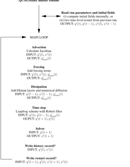
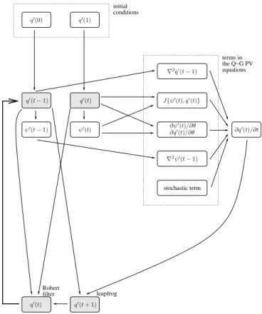
Given ψ_i′ and q_i′ at any time, we may evaluate ∂q_i′/∂t at that time using the prog-nostic Eqs. (23) and (24). There are contributions to the PPV tendency from advection (J(ψ_i′, q_i′)), forcing (∂/∂θ) and dissipation (∇2). We may use the tendency to determine q′_i at a short time in the future. We may then invert the diagnostic Helmholtz Eqs. (25)

5

and (26), in order to obtainψ_i′ at the future time. Finally, we may begin the loop again using the updated fields. This is how QUAGMIRE integrates the model equations.

The Helmholtz Eqs. (25) and (26), are coupled. The inversion is made easier by first re-writing them in vertical normal mode form in order to remove the coupling. We take the sum and difference of the equations to obtain, respectively,

10

∇2(ψ₁′ +ψ₂′)=q₁′ +q′₂ (31)

and

∇2(ψ₂′ ₋ψ₁′)₋Citcc

2f2

g′_H(ψ2′−ψ1′)=Citcc(q2′ −q′1), (32)

whereCitccis an interfacial tension correction coefficient given by

Citcc=

1

1−(2f2_δ2

m)/(g′H)

. (33)

15

We know thatf2δ_m2/g′H _≪ 1 (Sect. 3.1), and soC_itcc is slightly larger than unity, and is exactly equal to unity if the interfacial tension is zero.

Defining the barotropic (bt) and baroclinic (bc) vertical normal mode variables to be

Ψ′_bt=ψ₁′ +ψ₂′ , (34)

Ψ′_bc=ψ₂′ ₋ψ₁′ , (35)

20

Q_bt′ =q₁′ +q₂′ , (36)

Q′_bc=Citcc(q′2−q1′), (37)

(17)

GMDD

1, 187–241, 2008

QUAGMIRE v1.3

Title Page

Tables Figures

◭ ◮

Back Close

Full Screen / Esc

Interactive Discussion Eqs. (31) and (32) both become uncoupled Helmholtz equations of the form

∇2Ψ′m−λmΨ′m =Q′m , (38)

wherem=bt,bc. The eigenvalues areλbt=0 andλbc=2Citccf 2

/g′H.

We now perform a second normal mode decomposition, this time in the azimuthal dimension, in order to further simplify the solution of the Helmholtz equations. At each

5

time step, we expand

Ψ′m(r, θ)=

∞

X

n=−∞ ˆ Ψ′nm(r)e

√

−1nθ ₍₃₉₎

and

Q′_m(r, θ)= ∞

X

n=−∞ ˆ

Q′n_m(r)e√−1nθ. (40)

Since Ψ′m(r, θ) and Qm′ (r, θ) are real, the complex functions ˆΨ′ n

m and ˆQ′ n

m satisfy 10

ˆ

Ψ′nm=( ˆΨ′−mn)∗ and ˆQ′nm=( ˆQ′−mn)∗, where the asterisk represents complex conjugation.

The n=0 term is the mean flow correction, which is a correction to the mean flow that is generated by nonlinear self interactions of the waves. It is equal to the zonal average of the perturbation quantities, as can be seen from the zonal integration of Eqs. (39) and (40). Then6=0 terms represent wave (or eddy) components.

Substitut-15

ing Eqs. (39) and (40) into (38) gives the radial structure equation,

d2Ψˆ′nm

dr2 +

1 r

d ˆΨ′nm

dr − λm+ n2 r2

!

ˆ

Ψ′nm =Qˆ′nm(r). (41)

This complex ordinary differential equation must be solved for each combination of vertical modes, m ∈ {bt,bc}, and azimuthal modes, n ∈ {0,±1,±2, . . .}, in order to determine ˆΨ′nm(r) when given ˆQ′

n

m(r). The inversion process required in order to obtain 20

(18)

GMDD

1, 187–241, 2008

QUAGMIRE v1.3

Title Page

Tables Figures

◭ ◮

Back Close

Full Screen / Esc

Interactive Discussion q_i′ (36) & (37)_−→ Q′m

(40)

−→ Qˆ′n_m

↓

(41)

ψ_i′ (34) & (35)←− Ψ′m (39)

←− Ψˆ′nm

We could finally perform a third normal mode decomposition, this time in the radial dimension, by projecting ˆΨ′nm(r) and ˆQ′nm(r) onto the eigenfunctions of the linear

op-erator on the left side of Eq. (41). The baroclinic eigenfunctions are modified Bessel functions of order n in the scaled radial coordinate, ˜r=pλbcr (Boas, 1983) and the

5

barotropic eigenfunctions are of the formr±n. However, this approach would force the streamfunction and PPV to satisfy the same boundary conditions, for which there is no justification. QUAGMIRE therefore solves the radial structure equation directly rather than projecting onto the radial modes.

3.3 Perturbation streamfunction boundary conditions for the continuous equations

10

We must now choose boundary conditions to apply to the perturbation streamfunction when integrating Eq. (41). The equation was derived under the assumption of inviscid flow. Therefore, it cannot describe the thin, viscous Stewartson layers of widthδSwhich

exist at the lateral boundaries, and applies only to the fluid interior, a+δ_S<r<b−δ_S. We assume thatδ_S_≪a and δ_S_≪b so that we may still write the integration range as

15

a≤r≤b, but now when we refer tor=aorr=bwe mean the boundary between the fluid interior and Stewartson layer rather than the sidewall.

There are a number of possible boundary conditions. To impose passive Stewartson layers which do not anywhere exchange fluid with the interior, we would apply the impermeability condition to the radial perturbation velocity, i.e. u′_{i , r}|r=a, b=0, ∀ θ, i, 20

(19)

GMDD

1, 187–241, 2008

QUAGMIRE v1.3

Title Page

Tables Figures

◭ ◮

Back Close

Full Screen / Esc

Interactive Discussion which in the normal mode variables corresponds to Dirichlet boundary conditions,

ˆ

Ψ′nm|r=a, b=0, ∀n6=0, m . (42)

The mean flow correction velocity (n=0) is purely zonal and so automatically satisfies impermeability. Impermeability alone is therefore not a sufficient condition to uniquely specify a solution. No-slip boundary conditions for the zonal perturbation velocity,

5

i.e. u′_{i , θ}|r=a, b=0, ∀ θ, i, correspond in the normal mode variables to the Neumann

conditions,

d ˆΨ′nm

dr

_r

=a, b

=0, _∀n, m . (43)

The equilibrium solid-body rotation flow about which we perturb satisfies impermeabil-ity but does not satisfy the no-slip condition.

10

Since we are solving a second-order differential equation, only two independent boundary conditions are required. We cannot therefore impose both impermeability and no-slip flow at both boundaries, as that would require four independent conditions. The over-constrained nature of the PPV inversion in Q-G models has been discussed by Williams (1979). A comprehensive study of the comparative effects of using no-slip

15

boundary conditions, rather than the more traditional free-slip conditions, is described by Mundt et al. (1995).

We must use a reduced set of boundary conditions, but we must choose carefully and consistently which conditions to retain and which to abandon, in order to avoid non-physical behaviour. We are, of course, free to employ different boundary conditions for

20

the different normal mode components specified bymandn.

The debate over suitable lateral Q-G boundary conditions has had a long and con-tentious history in the literature. In the classic periodic channel models of Phillips (1954, 1956), Eq. (42) is applied to the wave (n6=0) components and Eq. (43) is ap-plied to the mean flow correction (n=0) component. The latter condition is not imposed

25

(20)

GMDD

1, 187–241, 2008

QUAGMIRE v1.3

Title Page

Tables Figures

◭ ◮

Back Close

Full Screen / Esc

Interactive Discussion shows that relaxing the mean flow correction boundary condition leads to a spurious,

unspecified energy flux through the sidewalls. The condition is included again by Ped-losky (1970), but replaced in PedPed-losky (1971) and PedPed-losky (1972) with an ad-hoc

condition chosen for mathematical convenience. Smith (1974) points out that the re-sulting non-physical energy source might invalidate Pedlosky’s results, and repeats

5

Pedlosky’s calculations with the proper boundary condition retained (Smith and Ped-losky, 1975; Smith, 1977). More recent studies (Appleby, 1982; Yoshida and Hart, 1986; Lewis, 1992; Stephen, 1998) have avoided the spurious energy flux by applying both conditions in full, as done by Phillips (1954, 1956).

An informative interpretation of Phillips’ mean flow correction boundary condition has

10

been given by Davey (1978). For non-zero zonal perturbation velocities,u′_{i , θ}|r=a, b, at

the boundary between the interior and a Stewartson layer, there will be a corresponding return volume flux between the Ekman layers and the Stewartson layer due to the asymmetry of the Ekman spiral (Pedlosky, 1987), which will have a non-zero radial component proportional to u′_{i , θ}|r=a, b. We can therefore ensure that there is no net 15

build-up of mass in the Stewartson layers by setting

Z2π

0

u′_{i , θ}|r=a, bdθ=0 ∀i . (44)

This condition is automatically satisfied for the wave (n₆₌0) components, and is equiv-alent to Eq. (43) withn=0, which is the condition used by Phillips. With this condition, there is nonet exchange of fluid due to the perturbation flow between each Ekman

20

layer and the Stewartson layers, althoughlocal exchange is allowed.

Next, we derive a consistent and plausible set of boundary conditions for the quasi-geostrophic annulus, which do not lead to non-physical behaviour, by considering inte-gral properties of the prognostic (Sect. 3.3.1) and diagnostic (Sect. 3.3.2) model equa-tions.

25

(21)

GMDD

1, 187–241, 2008

QUAGMIRE v1.3

Title Page

Tables Figures

◭ ◮

Back Close

Full Screen / Esc

Interactive Discussion 3.3.1 Integral properties of the prognostic equations

Consider the area-integral of the perturbation PPV tendencies over the annular domain,

Z2π

θ=0 Zb

r=a

∂q_i′

∂t rdrdθ , (45)

as given by the prognostic Eqs. (23) and (24). The forcing (∂/∂θ) terms integrate to give zero unconditionally. The advection (J(ψ_i′, q_i′)) terms integrate to give zero

5

(Salmon and Talley, 1989) if

∂ψ_i′ ∂θ

_r

=a, b

=0. (46)

The dissipation (_∇2) terms integrate to give zero if

Z2π

0

∂ψ_i′ ∂r

r=a, b

dθ=0. (47)

The conditions Eqs. (46) and (47) are equivalent to impermeability for the waves and

10

no-slip for the mean flow correction, as originally used by Phillips (1954, 1956). With these conditions, the horizontal-mean PPV in each layer is conserved by the continu-ous equations and there is no spuricontinu-ous energy flux. We choose to apply these condi-tions in QUAGMIRE, except that the latter condition leads to an ill-posed PPV inversion for the special case ofn=0 andm=bt, as we will now see.

15

3.3.2 Integral properties of the diagnostic equations

Equation (41) for the barotropic mean flow correction is

d2Ψˆ′0bt

dr2 +

1 r

d ˆΨ′0bt

dr =Qˆ ′0

(22)

GMDD

1, 187–241, 2008

QUAGMIRE v1.3

Full Screen / Esc

Interactive Discussion Since λbt=0 and n=0 for this case, one of the terms in the radial structure equation

has vanished, making the left side an exact derivative. Equation (48) can therefore be integrated analytically betweenr=aandr=bto give

bd ˆΨ ′0 bt dr

r=b

−ad ˆΨ ′0 bt dr

r=a

=

Zb

a

ˆ

Q′0_btrdr . (49)

In QUAGMIRE, we choose initial conditions for which the horizontal-mean barotropic

5

PPV is zero, and it is then guaranteed to remain zero at all times, as shown in Sect. 3.3.1. This means that we need only explicitly set

d ˆΨ′0bt

dr

r=a

=0 (50)

and we will automatically have

d ˆΨ′0bt

dr

r=b

=0, (51)

10

from Eq. (49). If we explicitly impose both Eq. (50) and Eq. (51) when solving Eq. (48), we will have an underconstrained and ill-posed problem. We need an additional con-straint to close the solution.

We have defined two streamfunctions in the model – one per layer, or equivalently, one per vertical normal mode – and each of these has an integration constant

asso-15

ciated with it (Sect. 3.1). Just because these two arbitrary constants have no physical meaning does not mean that they do not need to be defined in the numerical model. Now that we know that Eqs. (50) and (51) are not independent boundary conditions, and therefore that to explicitly impose both would lead to an underconstrained PPV inversion, we choose to explicitly impose only Eq. (50). We then take the opportunity to

20

use the remaining degree of freedom associated with the solution of Eq. (48) to define one of the streamfunction integration constants, by arbitrarily setting

ˆ

Ψ′0_bt|r=b=0, (52)

(23)

GMDD

1, 187–241, 2008

QUAGMIRE v1.3

Title Page

Tables Figures

◭ ◮

Back Close

Full Screen / Esc

Interactive Discussion which completes the set of two boundary conditions for them=bt,n=0 component, and

gives a well-posed problem.

Incidentally, the second streamfunction integration constant is defined by requiring the mean interface perturbation to be zero using Eq. (13), which follows from volume conservation for either layer. This requirement is imposed off-line, by adding a

suitably-5

chosen constant to one of the streamfunction fields when model diagnostics are plot-ted, and not as a boundary condition during the inversion.

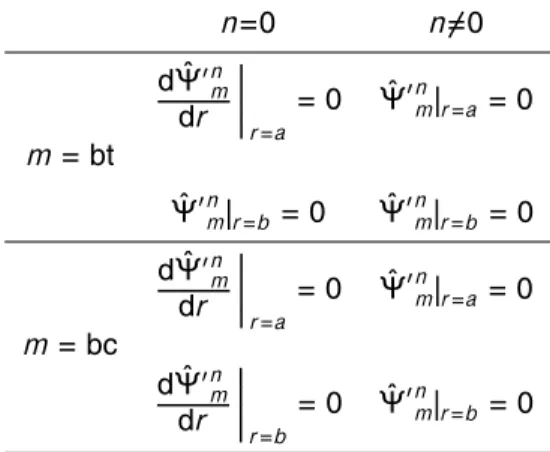
A summary of the boundary conditions which we must explicitly set when integrating Eq. (41) is given in Table 1. With these conditions, the sidewall boundaries are im-permeable to each component of the flow, i.e. the solid-body rotation equilibrium flow,

10

the mean flow correction and the wave components. The boundaries are slippery to the solid-body rotation flow and the wave components, but no-slip to the mean flow correction.

4 Discretized equations

We derived in Sect. 3 a set of partial differential equations and boundary conditions

15

which are both physically sensible and well-posed. We now discretize the equations so that they are suitable for numerical integration on a computer. We must take great care to ensure that the discretized equations and boundary conditions retain the important properties possessed by the continuous equations. In particular, it is important that they satisfy discretized analogues of the integral properties discussed in Sect. 3.3.

20

4.1 The numerical grid

(24)

GMDD

1, 187–241, 2008

QUAGMIRE v1.3

Title Page

Tables Figures

◭ ◮

Back Close

Full Screen / Esc

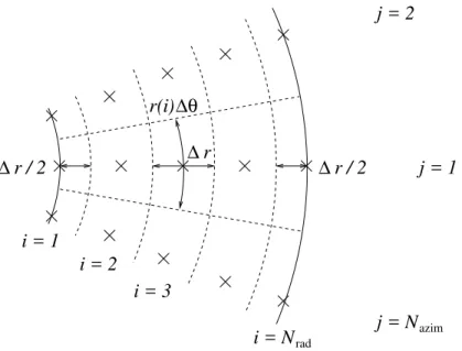
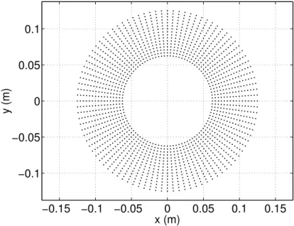
Interactive Discussion r=aandr=b) andNazim points in the azimuthal dimension. We define

∆r = b−a Nrad−1

(53)

and

∆θ= 2π

N_azim , (54)

and then we have

5

r(i)=a+(i₋1)∆r , i =1,2, . . . , Nrad (55)

and

θ(j)=j∆θ , j =1,2, . . . , Nazim. (56)

The point (i , Nazim+1) is identical to the point (i ,1). We define the perturbation

stream-functionψ′(i , j, k) and PPVq′(i , j, k) at each of these points in each layer (k=1,2), so

10

that ψ′ and q′ are co-located on the grid. The area of the grid box with coordinates (i , j) is approximately [1−1

2δi ,1−12δi , Nrad]r(i)∆r∆θ, whereδ∗,∗is the Kronecker delta

function.

4.2 Prognostic equations

In the continuous case, we chose perturbation streamfunction boundary conditions

15

such that each of the three contributions (advection, forcing and dissipation) to the area-integrated perturbation PPV tendency was zero. We would now like to choose discretizations of these contributions, together with discretizations of the boundary con-ditions, for which this statement still holdsexactly. If our discretization only conserves the mean PPV approximately, then there is the possibility of a non-physical and

ex-20

plosive increase in the PPV, even if the error is small, due to the compound effects of

(25)

GMDD

1, 187–241, 2008

QUAGMIRE v1.3

Title Page

Tables Figures

◭ ◮

Back Close

Full Screen / Esc

Interactive Discussion many time steps. Following Sect. 3.3.1, we therefore next examine the discretizations

and boundary conditions necessary to ensure that

N_rad X

i=1 N_azim

X

j=1

[1₋1 2δi ,1−

1

2δi ,Nrad]f(i , j, k)r(i)∆r∆θ=0 (57)

fork=1,2, wheref(i , j, k) is, in turn, the discretized azimuthal derivative, Jacobian and Laplacian.

5

The centred, second-order discretization of the azimuthal derivative,

f(i , j, k)= ψ

′_{(i , j} ₊_{1, k)}₋_ψ′_{(i , j} ₋_{1, k)}

2∆θ , (58)

satisfies Eq. (57) unconditionally, as in the continuous case.

The second-order Arakawa (1966) discretization of the Jacobian satisfies Eq. (57) if

ψ′(i , j+1, k)₋ψ′(i , j, k)

∆θ =0 ∀j, k, i =1, Nrad, (59)

10

which is a discretized version of the condition, Eq. (46), for the continuous case. It is tedious but straightforward to show that the five-point discretization of the Lapla-cian (whose continuous definition is given in Eq. 17 for reference),

f (i , j, k)

=ψ

′_(i₊_{1, j, k)}₋_2ψ′_{(i , j, k}₎₊_ψ′_(i ₋_{1, j, k)}

(∆r)2

15

+ψ

′_(i₊_{1, j, k)}₋_ψ′_(i ₋_{1, j, k)} 2r(i)∆r

+ψ

′_{(i , j}₊_{1, k)}₋_2ψ′_{(i , j, k}₎₊_ψ′_{(i , j} ₋_{1, k)}

[r(i)∆θ]2 , (60)

(26)

GMDD

1, 187–241, 2008

QUAGMIRE v1.3

Title Page

Tables Figures

◭ ◮

Back Close

Full Screen / Esc

Interactive Discussion ψ′(2, j, k)−ψ′(1, j, k)=ψ′(1, j, k)−ψ′(0, j, k) (61)

and

ψ′(Nrad+1, j, k)−ψ′(Nrad, j, k)=ψ′(Nrad, j, k)−ψ′(Nrad−1, j, k), (62)

satisfies Eq. (57) if

Nazim X

j=1

ψ′(2, j, k)−ψ′(1, j, k)

∆r =0 ∀k (63)

5

and

Nazim X

j=1

ψ′(Nrad, j, k)−ψ′(Nrad−1, j, k)

∆r =0 ∀k , (64)

which are discretized versions of the condition, Eq. (47), for the continuous case. There will be a small error in the value of the calculated discretized Laplacian at the bound-aries due to the assumption of linearly-extrapolated ghost points, but there is

appar-10

ently no other way to discretize the Laplacian in such a way that analogues of its integral properties are fully preserved.

4.3 Diagnostic equations

The discretized versions of Eqs. (39) and (40) are

Ψ′m(i , j)= N_azim−1

X

n=0

ˆ

Ψ′nm(i)e2π

√

−1nj /Nazim ₍₆₅₎

15

and

Q′_m(i , j)=

N_azim−1 X

n=0

ˆ

Q′n_m(i)e2π√−1nj /Nazim _. ₍₆₆₎

(27)

GMDD

1, 187–241, 2008

QUAGMIRE v1.3

Title Page

Tables Figures

◭ ◮

Back Close

Full Screen / Esc

Interactive Discussion The summations have been truncated, compared to Eqs. (39) and (40), because there

are onlyNazim independent Fourier components associated with the discrete Fourier

transform of a series ofNazimnumbers.

BecauseΨ′m(i , j) is real, we have

ˆ

Ψ′Nazim−n

m (i)=[ ˆΨ′nm(i)]∗ (67)

5

forn=1,2, . . . , Nazim−1. We chooseNazimto be even, and then we need only

explic-itly solve Eq. (41) forn=0,1,2, . . . , Nazim/2. Solutions for n=Nazim/2+1, Nazim/2+

2, . . . , Nazim−1 are given in terms of solutions forn=Nazim/2−1, Nazim/2−2, . . . ,1 by

Eq. (67), halving the processing time required for the PPV inversions. The maximum resolvable wavenumber is the Nyquist wavenumber,Nazim/2.

10

In terms of the normal mode variables, the discretized boundary conditions, (59), (63) and (64), reduce on substitution into Eqs. (65) and (66) to

ˆ

Ψ′nm(1) =0

ˆ

Ψ′nm(Nrad)=0

∀m, n₆₌0 (68)

and

ˆ

Ψ′0m(1) = Ψˆ ′ 0 m(2)

ˆ

Ψ′0m(Nrad)=Ψˆ′ 0

m(Nrad−1) )

∀m . (69)

15

We now consider the discretization of the radial structure Eq. (41). Using centred three-point finite differences at the interior points,i=2,3, . . . , Nrad−1, we obtain

ˆ

Ψ′nm(i−1)−2 ˆΨ′mn(i)+Ψˆ′nm(i+1)

(∆r)2 +

ˆ

Ψ′nm(i+1)−Ψˆ′nm(i−1) 2r(i)∆r −

"

λm+

n2

[r(i)]2 #

ˆ

Ψ′nm(i)=Qˆ′nm(i). (70) Re-grouping terms according to grid points gives

(28)

GMDD

1, 187–241, 2008

QUAGMIRE v1.3

Full Screen / Esc

Interactive Discussion where the dimensionless quantitiesα±andγ are given by

α±(i)=1_± ∆r

2r(i) (72)

and

γ(i)=−2₋

"

λ_m+ n

2

[r(i)]2 #

(∆r)2. (73)

In Cartesian geometry we would haveα±(i)=1.

5

TheNrad−2 equations, Eq. (71), together with 2 boundary conditions, complete the

set ofNrad equations in the Nrad unknowns, ˆΨ′ n

m(i) fori=1,2, . . . , Nrad. These linear

equations may be written in matrix form,

        

bdy bdy _{· · ·} α−(2) γ(2) α+(2) · · · α−(3) γ(3) α+(3) · · · α−(4) γ(4) α+(4) _{· · ·} α−(5) γ(5) _{· · ·} .. . ... ... ... ... . ..          ×          ˆ Ψ′nm(1)

ˆ Ψ′nm(2)

ˆ Ψ′nm(3)

ˆ Ψ′nm(4)

ˆ Ψ′nm(5)

.. .          =           0 ˆ

Q′n_m(2)(∆r)2 ˆ

Q′nm(3)(∆r)2

ˆ

Q′nm(4)(∆r) 2

ˆ

Q′n_m(5)(∆r)2 .. .           , (74)

where the zero elements in the tridiagonalNrad×Nradmatrix have been left blank. The

10

two elements labelled “bdy” are boundary condition elements, dependent uponmand n. There are two further such elements in the right-most two columns of the bottom row.

4.4 Perturbation streamfunction boundary conditions for the discretized equations

In the continuous case, we found that the boundary conditions for the barotropic mean

15

flow correction component (m=bt, n=0) were ill-posed as originally stated, and re-mained so until we replaced a redundant boundary condition with an equation to define

(29)

GMDD

1, 187–241, 2008

QUAGMIRE v1.3

Title Page

Tables Figures

◭ ◮

Back Close

Full Screen / Esc

Interactive Discussion an integration constant. This happens in the discretized case, too: the square matrix

in Eq. (74) is singular for the barotropic mean flow correction, when the boundary con-dition elements (labelled “bdy”) are (−1,1) in the top row and (1,−1) in the bottom row. The analytical proof of this, which involves showing that a certain linear combination of rows is zero, is tedious but straightforward. By analogy with the continuous case,

5

we replace the two boundary condition elements in the bottom row with (0,1) to define the integration constant by setting the streamfunction for this component to zero on the outer boundary, and then the matrix is no longer singular.

In the continuous system, we set then=0,m=bt normal streamfunction derivative to zero at one boundary and found that, if the mean barotropic PPV was zero, the

stream-10

function derivative would automatically be zero at the other boundary. Importantly, in contrast with the continuous system, this statement does not hold exactly for the dis-cretized system. This is because ˆQ′n_m(1) and ˆQ′n_m(Nrad) do not appear in Eq. (74): we

do not apply the discretized differential equation at the boundaries, because we need to use these two degrees of freedom to impose the boundary conditions.

15

The error corresponding to this PPV leak is small, but even small errors can grow to dominate the solution after a large number of time steps. To fix this problem with the barotropic mean flow correction, we discard the outer boundary streamfunction,

ˆ

Ψ′0bt(Nrad), obtained through inversion of Eq. (74) and define a new value for it by setting

ˆ

Ψ′0bt(Nrad)=Ψˆ ′ 0

bt(Nrad−1). This ensures that the boundary conditions, Eq. (69), required

20

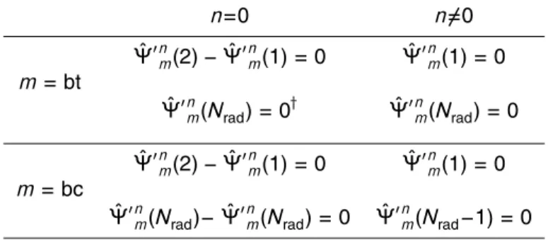
for conservation of horizontal-mean PPV are satisfied exactly. The consequence is that the discretized differential equation, Eq. (70), is not exactly satisfied at the pointNrad−1.

The imposed boundary conditions are summarized in Table 2.

4.5 Relaxation

Instead of (or in addition to) the mechanical forcing imposed by the differentially

rotat-25

(30)

GMDD

1, 187–241, 2008

QUAGMIRE v1.3

Title Page

Tables Figures

◭ ◮

Back Close

Full Screen / Esc

Interactive Discussion the relaxation perturbation streamfunction is used in the computation of the diffusion

and hyperdiffusion terms. If relaxation to a specified perturbation potential vorticity is activated, then the perturbation potential vorticity is relaxed towards the relaxation perturbation potential vorticity at a prescribed rate.

4.6 Numerical methods

5

We now discuss the time-stepping scheme (Sect. 4.6.1), the need for time-lagged dif-fusion (Sect. 4.6.2), and the approximate representation of unresolved features using hyperdiffusion (Sect. 4.6.3) and stochastic forcing (Sect. 4.6.4).

4.6.1 Time stepping

For the time stepping we use a leapfrog scheme with a Robert (1966) three-level time

10

filter applied at each time step, to suppress the computational mode splitting between even and odd steps (Mesinger and Arakawa, 1976). At each step, of size∆t,qt+1is determined at each grid point using the leapfrog scheme,

qt+1=qt−1+2∆t qt_tendency, (75)

and then the value ofqt is adjusted in such a way as to move it closer to the mean of

15

qt−1andqt+1, according to

qt→qt+R q

t₋1

+qt+1 2 −q

t !

. (76)

The old value ofqt is abandoned and the new, filtered value is used in its place. The Robert filter parameter,R>0, is chosen to be as small as possible whilst still suppress-ing the leapfrog decouplsuppress-ing.

20

(31)

GMDD

1, 187–241, 2008

QUAGMIRE v1.3

Title Page

Tables Figures

◭ ◮

Back Close

Full Screen / Esc

Interactive Discussion 4.6.2 Time-lagged diffusion

Numerical solutions of the simple diffusion equation, using the leapfrog scheme for the time discretization and a time-centred, three-point finite difference for the space discretization, are unconditionally unstable due to a computational mode (Haltiner and Williams, 1980). To avoid this in QUAGMIRE, we time-lag the diffusion terms by one

5

time step when evaluating the right sides of the discretized analogues of Eqs. (23) and (24). This means that, when evaluating the PPV tendency, we calculate the forcing (∂/∂θ) and advection (J(ψ_i′, q_i′)) terms using the fields at the current time step, but we calculate the diffusion (_∇2) terms using the fields at the previous time step.

4.6.3 Hyperdiffusion

10

To represent sub-gridscale effects we add a hyperdiffusion term to the right sides of the prognostic Eqs. (23) and (24), as is usual in numerical models (e.g. Lewis, 1992).

At first, a fourth-order streamfunction hyperdiffusion term, ν_hyper_∇4ψ_i′, was tested, but significant grid-scale features were always found to form at the lateral boundaries whenever the model was run. This is because during the PPV inversion, any

grid-15

scale features in the PPV field will give rise to corresponding grid-scale features in the perturbation streamfunction field, and then theνhyper∇

4

ψ′ contribution to the PPV tendency will tend to damp out these features in the PPV field. Unfortunately this does not happen at the boundaries in the discretized system, because boundary values of the PPV are not used when performing the inversion: as already discussed, ˆQ′nm(1) 20

and ˆQ′n_m(Nrad) are missing from Eq. (74). Values of PPV are able to feed back into the

PPV tendency field only at interior points, and there is nothing to suppress grid-scale features in the PPV field at the boundaries.

To avoid this, we instead use second-order hyperdiffusion applied to the PPV, by adding a termνhyper∇

2

q′_i to the prognostic equations. This term is also time-lagged by

25

(32)

GMDD

1, 187–241, 2008

QUAGMIRE v1.3

Title Page

Tables Figures

◭ ◮

Back Close

Full Screen / Esc

Interactive Discussion possible to the exact solutions, we periodically reset the horizontal-mean PPV to zero

in QUAGMIRE, by adding a very small constant whose value is chosen to satisfy this requirement.

4.6.4 Stochastic parameterization of sub-gridscale effects

As an alternative method for representing sub-gridscale effects, there is the option

5

of a simple stochastic parameterization in QUAGMIRE. Such parameterizations are increasingly used in numerical models, with the recognition that the additional degrees of freedom they introduce may be able to compensate, at least partially, for the degrees of freedom missing from filtered models (e.g. Williams et al., 2004).

We choose the simplest possible form for the noise terms. At each grid point and at

10

each time step, a random number is drawn from the uniform distribution on the interval [0,1], and then shifted to the interval [₋amp,amp] before being used as an additive contribution to the PPV tendency. At each grid point and at each time step, the added random number is equal and opposite in the upper and lower layers, nominally repre-senting pure-baroclinic inertia-gravity waves. The constant, amp, is a given amplitude

15

with units s−2, which may change linearly with time in the model. The noise contains no correlations in either time or horizontal position. The horizontal-mean random number field is enforced to be zero in both layers.

4.7 Initial conditions

A feature of the leapfrog time-stepping scheme is that initial condition fields are

re-20

quired at two consecutive times, in order to begin the integration. We choose to specify the PPV fields as initial conditions. We use small amplitude random noise for these fields, seeding the system to permit the growth of unstable perturbations of any az-imuthal and radial wavenumber. We generate random numbers from a uniform distri-bution, which we then shift to a chosen symmetrical interval centred on zero. We then

25

subtract the mean PPV in each layer at both time steps, which makes the fields satisfy