www.geosci-instrum-method-data-syst.net/3/187/2014/ doi:10.5194/gi-3-187-2014
© Author(s) 2014. CC Attribution 3.0 License.
A framework for benchmarking of homogenisation
algorithm performance on the global scale
K. Willett1, C. Williams2, I. T. Jolliffe3, R. Lund4, L. V. Alexander5, S. Brönnimann6, L. A. Vincent7, S. Easterbrook8, V. K. C. Venema9, D. Berry10, R. E. Warren11, G. Lopardo12, R. Auchmann6, E. Aguilar13, M. J. Menne2,
C. Gallagher4, Z. Hausfather14, T. Thorarinsdottir15, and P. W. Thorne16
1Met Office Hadley Centre, FitzRoy Road, Exeter, UK 2National Climatic Data Center, Ashville, NC, USA 3Exeter Climate Systems, University of Exeter, Exeter, UK
4Department of Mathematical Sciences, Clemson University, Clemson, SC, USA
5ARC Centre of Excellence for Climate System Science and Climate Change Research Centre,
University of New South Wales, Sydney, Australia
6Oeschger Center for Climate Change Research & Institute of Geography, University of Bern, Bern, Switzerland 7Climate Research Division, Science and Technology Branch, Environment Canada, Toronto, Canada
8Department of Computer Science, University of Toronto, Toronto, Canada 9Meteorologisches Institut, University of Bonn, Bonn, Germany
10National Oceanography Centre, Southampton, UK
11College of Engineering, Mathematics and Physical Sciences, University of Exeter, Exeter, UK 12Istituto Nazionale di Ricerca Metrologica (INRiM), Torino, Italy
13Centre for Climate Change, Universitat Rovira i Virgili, Tarragona, Spain 14Berkeley Earth, Berkeley, CA, USA
15Norwegian Computing Center, Oslo, Norway
16Nansen Environmental and Remote Sensing Center, Bergen, Norway
Correspondence to:K. Willett ([email protected])
Received: 27 February 2014 – Published in Geosci. Instrum. Method. Data Syst. Discuss.: 4 June 2014 Revised: 21 August 2014 – Accepted: 30 August 2014 – Published: 25 September 2014
Abstract. The International Surface Temperature Initiative (ISTI) is striving towards substantively improving our abil-ity to robustly understand historical land surface air temper-ature change at all scales. A key recently completed first step has been collating all available records into a comprehensive open access, traceable and version-controlled databank. The crucial next step is to maximise the value of the collated data through a robust international framework of benchmarking and assessment for product intercomparison and uncertainty estimation. We focus on uncertainties arising from the pres-ence of inhomogeneities in monthly mean land surface tem-perature data and the varied methodological choices made by various groups in building homogeneous temperature prod-ucts. The central facet of the benchmarking process is the creation of global-scale synthetic analogues to the real-world
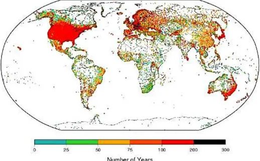
Figure 1.Station locations coloured by length of record for version1 of the ISTI Land Meteorological Databank stage 3 (recommended merged version) version 1.0.0 (source: Fig. 8 in Rennie et al., 2014).
1 Introduction
Monitoring and understanding our changing climate requires freely available data with good spatial and temporal cover-age that is of high quality, with the remaining uncertain-ties well quantified. The International Surface Temperature Initiative (ISTI; www.surfacetemperatures.org; Thorne et al., 2011) is striving towards substantively improving our ability to robustly understand historical land surface air temperature change at all scales. A key recently completed first step has been collating all known freely available land surface me-teorological records into an open access, traceable to known origin where possible, and version controlled databank (Ren-nie et al., 2014). To date the focus has been on monthly tem-perature time series, so far achieving a database of just over 32 000 unique records in the first release version as it stood on 20 June 2014 (Fig. 1).
There are multiple additional processes that must be performed to transform these fundamental data holdings into high-quality-data products that are suitable for robust climate research, henceforth referred to as climate data records (CDRs). These processes include: quality control, homogenisation, averaging, and in some cases interpolation. At present, a number of independent climate data groups maintain CDRs of land surface air temperature. These can range from data sets at global, regional or national/local scales of single stations or gridded products. Each uses its own choice of methods to process data from the raw observa-tions to a CDR. In most cases, these methods are automated, given the large number of stations, and purely statistical due to poor metadata availability.
ISTI’s second programmatic focus is to set up a framework to evaluate these methodological choices that ultimately lead to structural uncertainties in the trends and variability from CDRs. In particular, the ISTI focuses on homogenisation al-gorithm skill. This can be tested using a set of synthetic temperature records, analogous to real station networks but where inhomogeneities have deliberately been added. As such, the “truth” about where and what errors exist is known a priori. The ability of the algorithm to locate the change points and adjust for the inhomogeneity, ideally returning the “truth”, can then be measured. This community-based vali-dation on a realistic problem is referred to as benchmarking henceforth.
Unfortunately, change has been ubiquitous for the majority of station records (e.g. Lawrimore et al., 2011; Rohde et al., 2013). The dates of these changes (known as change points) are in many (very likely most) cases unknown and their im-pacts (known as inhomogeneities) either poorly quantified or more often than not entirely unquantified at source, neces-sitating subsequent analysis for change points and resulting inhomogeneities by third party analysts.
Climate observations made at individual stations exhibit multi-timescale variability made up of annual to decadal variations, seasonality and weather, all modulated by the sta-tion’s microclimate. Inhomogeneities can arise for a number of reasons such as station moves, instrument changes and changes in their exposure (shelter change), changes to the surrounding environment and changes to observing/reporting practices. While in the simplest cases a station may have one abrupt inhomogeneity in the middle of its series, which is rel-atively easy to detect, the situation can be far more complex with multiple change points caused by a number of diverse inhomogeneities. For example, inhomogeneities may be:
– geographically or temporally clustered due to events which affect entire networks or regions (e.g. change in observation time)
– close to end points of time series – gradual or sudden
– variance-altering
– combined with the presence of a long-term background trend
– small – frequent
– seasonally or diurnally varying
and often a combination of the above. A good overview of in-homogeneities in temperature and their causes can be found in Trewin (2010). Identifying the correct date (change point) and magnitude for any inhomogeneity against background noise is difficult, especially if it varies seasonally. Even after detection a series of decisions are required as to whether and how to adjust the data. While decisions are as evidence-based as possible, some are unavoidably ambiguous and can have a further non-negligible impact upon the resulting data. This is especially problematic for large data sets where the whole process by necessity is automated.
In this context attaining station homogeneity is very dif-ficult; many algorithms exist with varying strengths, weak-nesses and levels of skill (detailed reviews are presented in Venema et al., 2012, Aguilar et al., 2003, and Peterson et al., 1998). Many are already employed to build global and regional temperature products (CDRs) routinely used in cli-mate research (e.g. Xu et al., 2013; Trewin, 2013; Vincent et
al., 2012; Menne et al., 2009). While these algorithms can improve the homogeneity of the data, both spatially and tem-porally, some degree of uncertainty is extremely likely to remain (Venema et al.,2012) depending on methodological choices. Narrowing these bands of uncertainty is highly un-likely to change the story of increasing global average tem-perature since the late 19th century. However, large-scale biases could be reduced (Williams Jr. et al., 2012) and es-timates of temperature trends at regional and local scales, while becoming spatially more consistent, could be greatly affected.
The only way to categorically measure the skill of a ho-mogenisation algorithm for realistic conditions is to test it against a benchmark. Test data sets for previous benchmark-ing efforts have included one or more of the followbenchmark-ing: as homogeneous as possible real data, synthetic data with added inhomogeneities, or real data with known inhomo-geneities. Although valuable, station test cases are often rel-atively few in number (e.g. Easterling and Peterson, 1995) or lacking real-world complexity of both climate variabil-ity and inhomogenevariabil-ity characteristics (e.g. Vincent, 1998; Ducré-Robitaille et al., 2003; Reeves et al., 2007; Wang et al., 2007; Wang, 2008a, b). A relatively comprehensive but regionally limited study is that of Begert et al. (2008), who used the manually homogenised Swiss network as a test case. The European homogenisation community (the HOME project; www.homogenisation.org; Venema et al., 2012) is the most comprehensive benchmarking exercise to date. HOME used stochastic simulation to generate realistic net-works of ∼100 European temperature and precipitation records. Their probability distribution, cross- and autocorre-lations were reproduced using a “surrogate data approach” (Venema et al., 2006). Inhomogeneities were added such that all stations contained multiple change points and the magnitudes of the inhomogeneities were drawn from a nor-mal distribution. Thus, snor-mall undetectable inhomogeneities were also present, which influenced the detection and justment of larger inhomogeneities. Those methods that ad-dressed the presence of multiple change points within a se-ries (e.g. Caussinus and Lyazrhi, 1997, Lu et al., 2010; Han-nart and Naveau, 2012; Lindau and Venema, 2013) and the presence of change points within the reference series used in relative homogenisation (e.g. Caussinus and Mestre, 2004; Menne and Williams, 2005, 2009; Domonkos et al., 2011) clearly performed best in the HOME benchmark.
The ISTI benchmarks should lead to significant advance-ment over what is currently available. They will be global in scale, offer a better representation of real-world complex-ity both in terms of station characteristics and inhomogene-ity characteristics and provide a repeatable internationally agreed assessment system. The requirement for homogeni-sation benchmarks is becoming increasingly important, be-cause policy decisions of enormous societal and economic importance are now being based on conclusions drawn from observational data. In addition to underpinning our level of confidence in the observations, developing and engendering a comprehensive and internationally recognised benchmark system would provide three key scientific benefits:
1. objective intercomparison of data-products
2. quantification of the potential structural uncertainty of any one product
3. a valuable tool for advancing algorithm development. The Benchmarking and Assessment Working Group was set up during the Exeter, UK, 2010 workshop for the ISTI to develop and oversee the benchmarking pro-cess for homogenisation of temperature products. Further details can be found at www.surfacetemperatures.org/ benchmarking-and-assessment-working-group and blog discussions can be found at http://surftempbenchmarking. blogspot.com. The Benchmarking and Assessment Work-ing Group reports to the SteerWork-ing Committee and is guided by the Benchmarking and Assessment Terms of Reference hosted at www.surfacetemperatures.org/ benchmarking-and-assessment-working-group.
The objective of this paper is to lay out the basic frame-work for developing the first comprehensive benchmarking system for homogenisation of monthly land surface air tem-perature records on the global scale. By defining what we be-lieve a global homogenisation benchmarking system should look like, this paper is intended to serve multiple aims. Firstly, it provides an opportunity for the global community to provide critical feedback. Secondly, the document serves as a reference for our own purposes and others wishing to develop benchmarking systems for other parameters of prob-lems of a similar nature. Finally, it constitutes a basis for further improvement down the line as knowledge improves. Future papers will provide detailed methodologies for the various components of the benchmarking system described herein.
Here, the focus is solely on monthly mean temperatures. These concepts broadly apply to daily or subdaily scales and additional variables (e.g. maximum temperature, minimum temperature, diurnal temperature range). However, both de-velopment of synthetic data and implementation of realis-tic inhomogeneities, while maintaining physical consistency across different variables simultaneously, requires signifi-cantly increased levels of complexity.
The creation of spatio-temporally realistic analogue sta-tion data is discussed in Sect. 2. The development of real-istic, but optimally assessable error models is discussed in Sect. 3. An assessment system that meets both the needs of algorithm developers and data-product users is explored in Sect. 4. A proposed benchmarking cycle to serve the needs of science and policy is described in Sect. 5. Section 6 con-tains concluding remarks.
2 Reproducing “real-world” data – the analogue-clean worlds
Simple synthetic analogue-station data with simple inho-mogeneities applied may artificially award a high perfor-mance to algorithms that cannot cope with real-world data. A true test of algorithm skill requires global reconstruction of real-world characteristics including space and time sam-pling of the observational network. Hence, the ISTI bench-marks should replicate the spatio-temporal structure of the ∼32 000 stations in the ISTI databank stage 3 as far as pos-sible (http://www.surfacetemperatures.org/databank; Rennie et al., 2014) available from ftp://ftp.ncdc.noaa.gov/pub/data/ globaldatabank/monthly/stage3/.
The benchmark data must have realistic trends, variability, station autocorrelation and spatial cross-correlation. Concep-tually, we consider individual station temporal variability of ambient temperaturexat sitesand timetas being able to be decomposed as
xt,s=ct,s+lt,s+vt,s +mt,s, (1)
where:
– crepresents the unique station climatology (the deter-ministic seasonal cycle). This will vary even locally due to the effects of topography, land surface type and any seasonal cycle of vegetation.
– lrepresents any long-term trend (not necessarily linear, with possible seasonally varying components) that is ex-perienced by the site due to climatic fluctuations such as in response to external forcings of the global climate system.
– mrepresents the station microclimate (local variability). Such station-specific deviations are oftentimes weakly autocorrelated and cross-correlated with nearby sta-tions, but tend to be more distinct on a station-by-station basis than the remaining terms in Eq. (1).
These terms are assumed to be additive in this conceptual framework. This equation should not be considered to be a formal mathematical representation. All four components are deemed necessary to be able to subsequently build realistic series of xt,s on a network-wide basis that retain plausible
station series, neighbour series and regional series. Below, a discursive description of the necessary steps and build-ing blocks envisaged is given. A variety of methodological choices could be made when building the analogue-clean worlds. It is envisaged that the sophistication of methods will develop over time, improving the real-world representative-ness of the benchmarks periodically.
Station-neighbour cross-correlations depend on more than distance, such as differences in elevation, aspect, continen-tality and land use. If real-world data are used to formu-late all or part of a model to synthetically recreate station data, we need to be sure that errors within the real data (ran-dom or systematic) are not characterised and reproduced by the model. Ultimately, while analogue-clean world month-to-month station temperatures need not be identical to real station temperatures, realistic station climatology, variability, trends, autocorrelation and cross-correlation with neighbours should be maintained. Analogue-clean-world station tempo-ral sampling can be degraded to varying levels of missing data as necessary.
Most algorithms analyse the difference between a candi-date station and a reference station (or composite). Crucially, temperature climate anomalies (where the seasonal cycle,c, has been removed) are used to create the difference series. The large-scale trend,l, and variability,v, are highly corre-lated between candidate and reference series and so mostly removed by the differencing process. It is thus critical that the variability, autocorrelation and spatial cross-correlations inmare realistic, and hence the variability and autocorrela-tion in staautocorrela-tion-reference difference series are realistic.
For the benchmarking process, global climate models (GCMs) can provide gridded values of l (and possibly v) for monthly mean temperature. GCMs simulate the global climate using mathematical equations representing the basic laws of physics. GCMs can therefore represent plausible esti-mates of the short- and longer-term behaviour of the climate system resulting from solar variations, volcanic eruptions and anthropogenic changes (external forcings). They can also potentially represent natural large-scale climate modes (e.g. El Niño–Southern Oscillation – ENSO) and associated teleconnections (internal variability). However, the gridded nature of GCM output means that GCMs cannot give a suf-ficiently realistic representation of fine-scale meteorological data at point (station) scales. Hence, they cannot be used
di-rectly to provide themandccomponents at the point (sta-tion) level. Thelandvcomponents are expected to vary very little between stations that are close (e.g. within a grid box) and can reasonably be obtained by simple interpolation of GCM grid box values to point location.
There are three advantages of using GCMs to providel and v. Firstly, they provide globally consistent variability that can be associated with ENSO-type events or other real modes of variability with large spatial influence along with at least broad-scale topography (elevation, aspect, proxim-ity to the coast, etc.) and its influence. Secondly, time se-ries from a GCM will be free from inhomogeneity. Thirdly, there are different forcing scenarios available (e.g. no anthro-pogenic emissions, very high anthroanthro-pogenic emissions) pro-viding opportunities to explore how different levels of back-ground climate change affect the homogenisation algorithm skill. Note that background trends may be seasonally variant, further complicating seasonally varying inhomogeneity de-tection. Such characteristics may be obtainable from a GCM. The annually constantccomponent in Eq. (1) is straight-forward to calculate for each real station and then apply to the synthetic stations. Themandv (if not obtained from a GCM) component can be modelled statistically from the be-haviour of the real station data, taking care to account for sta-tion inhomogeneity and not include it in the statistical model. Statistical methods such as vector-autoregressive (VAR)-type models (e.g. Brockwell and Davis, 2006) can reproduce the spatio-temporal correlations but limitations exist where sta-tion records are insufficiently long or stable enough to be modelled. Balancing sophistication of methods with automa-tion and capacity to run on∼32 000 stations is key. Ensuring spatial consistency across large distances (hundreds of kilo-metres) necessitates high-dimensional-matrix computations or robust overlapping window techniques.
The key measures of whether benchmark clean worlds are good enough are as follows:
– station to neighbour cross-correlation
– standard deviation and autocorrelation of station minus neighbour difference series (of climate anomalies) – station autocorrelation.
These measures should be compared between real networks that we know to be of high quality (relatively free from ran-dom and systematic error) such as NOAA’s USCRN (United States Climate Reference Network; http://www.ncdc.noaa. gov/crn/) and the collocated analogue-clean world stations.
3 Devising realistic but optimally assessable error models – the analogue-error worlds
Ideally each analogue-error world would be based on a dif-ferent analogue-clean world to prevent prior knowledge of the “truth” (analogue-clean world). These error models should be designed with the three aims of the ISTI in mind, i.e. to aid product intercomparison, to help quantify structural uncertainty, and to aid methodological advancement. There should be blind benchmarks, where the answers/analogue-clean worlds underlying the released analogue-error worlds will not be made public for a time. Additionally, there should be some open benchmarks, where the answers/analogue-clean worlds will be publicly available immediately.
Blind benchmarksshould be used for formal assessment of algorithms and data products. By being blind they pre-vent optimisation to specific features. While certain fea-tures will be widely known, it should not be known which world explores which type of features or the exact change point/inhomogeneity magnitude. For the most part these blind worlds should be physically plausible scenarios based on our understanding of real-world issues. The inclusion of a control case of a homogeneous world will enable assess-ing the effect of false detections and the potential for algo-rithms to do more harm than good. Ultimately, they should be designed to lead to clear and useful results, distinguishing strengths and weaknesses of algorithms against specific in-homogeneity and climate data characteristics. They need to achieve this without completely overloading algorithm cre-ators from the outset, either with a multitude of complexities in all cases or with too many analogue-error worlds to con-tend with.
The open benchmarks will enable algorithm developers to conduct their own immediate tests comparing their ho-mogenised efforts from the analogue-error worlds with the corresponding analogue-clean worlds. These open worlds will also be useful for exploring some of the more exotic problems or alternatively those straightforward issues that do not require a full global station database to explore.
Systematic errors are the key problem for station homo-geneity and the prime focus for these benchmarks. These are persistent offsets or long-term trends away from the true am-bient temperature (metrologically speaking, an artefact that causes the measurement to differ in a sustained manner from the true value of the measurand). Random errors are also prevalent in many observational records. These arise from isolated instrument faults or observer/transmission and col-lation mistakes. For monthly averages, random errors at ob-servation times will often average out. Given a reasonable level of quality control, an essential step in any CDR process-ing, these errors are not thought to impact long-term-trend assessment although for individual stations this may not be the case.
To ensure focus on homogenisation methods, at least the first benchmark cycle should include only systematic errors and not random errors. Hence, users will not be required to quality control the analogue-error worlds although they are strongly recommended to quality control the real ISTI
data-bank. We note that in some cases a change point may be preceded by a systematic increase in random error – for ex-ample, an instrument or shelter could deteriorate gradually until a point at which it is replaced. In future versions of the benchmarks, specific error worlds could include known types of random errors to test how this affects the homogenisation algorithm skill.
Themes of different systematic inhomogeneities can be added to the analogue-clean world stations to create in-homogeneous analogue-error worlds. Conceptually, for any analogue-stationx as denoted by Eq. (1) a d term can be added to represent an inhomogeneity at time t and site s to give an observed value x′ which differs from the true value (x):
xt,′s =ct,s +lt,s +vt,s+mt,s+dt,s. (2)
At any point in time,dmay be zero, a constant (possibly with some seasonal or climate-related variation; e.g. an instrument change may yield a warm bias in winter and a cool bias in summer if not well ventilated) or a value that grows/declines over time as e.g. a tree grows or urban areas encroach. A growingd term may be smooth or jumpy. Experience with current benchmarks over restricted regions (Williams et al., 2012; Venema et al., 2012) suggests that several artefacts ex-ist in most station records such that thedt,sterm may change
several times during the period of record of a station (roughly every 10–30 years or more often).
In a perfect case, a homogenisation algorithm would de-tectd in the analogue-error world correctly, remove it, and adjustx′to its true ambient temperaturex from the original analogue-clean world (Eq. 1). By necessity, homogenisation algorithms have to make an assumption that a given station is at least locally representative at some point in its record. For convenience, and because the major interest is change in temperature rather than actual temperature, the most recently observed period is treated as the reference period by the ma-jority of algorithms. Any adjustments are made relative to this period. This creates issues for a user interested in the actual temperature because for any one station the period of highest absolute accuracy may not be the most recent period. However, it is not really possible to detect which period is the most accurate for each station and having multiple refer-ence periods in the benchmarks would make assessment far more complex and less useful. Hence, our assessment will assume all stations are representative in the most recent part of their record such thatdis zero at present day and additive backwards.
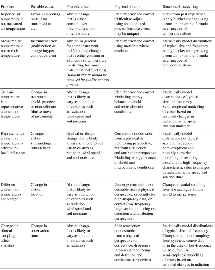
Table 1.Known inhomogeneities between observed air temperature and the ambient air temperature representative of a given location in terms of problems, possible causes and effects, physical solutions, and possible implementations in modelling a benchmark.
Problem Possible cause Possible effect Physical solution Benchmark modelling
Reported air Errors in reporting, Abrupt change Identify error and correct Draw from past experience. temperature is units, data that is either (difficult to adjust Apply blanket changes using not measured transmission, constant over using an automated a constant or simple formula air temperature etc. time or a function process because errors as a function of
of temperature may be unique) temperature alone
Measured air Instrument error Abrupt (or gradual Identify error and correct, Statistically model distributions temperature is (malfunction or for some instrument using metadata where of typical size and frequency. not true air change intype), malfunctions) change available Apply blanket changes using temperature calibration error that is either constant or a constant or simple formula
a function of temperature as a function of
(or drifting for some temperature alone
instrument malfunctions) (random errors should be removed by quality-control process)
True air Change in Abrupt change Identify error and correct. Statistically model temperature instrument that is likely to Modelling energy distributions of typical is not shield, practice vary as a function balance of shield size and frequency. representative or microclimate of variables such and microclimatic Semi-empirical modelling
ambient air (due to move as radiation, conditions of errors based on
temperature of instrument) wind speed and assumed changes in
soil moisture radiation, wind speed
and soil moisture
Representative Changes in Gradual or abrupt Correction not desirable Statistically model ambient air station change that is likely from a physical or distributions of typical temperature is surroundings, to vary as a function of monitoring perspective, size and frequency. affected by urbanisation variables such as but from a detection Semi-empirical and local influences radiation, wind speed and attribution perspective. possibly numerical
and soil moisture Modelling energy balance modelling of resulting of shield and trend and its high-frequency microclimatic conditions characteristics due to changes
in radiation, wind speed and soil moisture
Different Change in Abrupt change Unmerge (correction not Change in spatial sampling ambient air station that is likely to desirable from a physical from the analogue-known temperatures location vary as a function perspective, especially for world to merge series
are merged of variables such high-frequency data) or
as radiation, correct (low-frequency wind speed and large-scale monitoring and soil moisture detection and attribution
perspective)
Changes in Change in Abrupt change Split (correction Statistically model distributions
diurnal observation that is likely to not desirable of typical size and frequency.
sampling time vary as a function from a physical Change in temporal sampling
affect of variables such perspective) or from synthetic source data
statistics as radiation correct (low-frequency or in the case of low-frequency
large-scale monitoring GCM output use and detection and semi-empirical modelling attribution perspective) of errors based on
should be taken into account if possible. Given the current state of knowledge this will in many respects be an as-sumption based on expert judgement. Many complicated ex-amples of covariate impacts on d exist. For example, in soil-moisture-limited regions changing vegetation between wet years and dry years increases variability compared to a more constant soil-moisture environment (B. Trewin, per-sonal communication, 2013; Seneviratne et al., 2012).
Inhomogeneities added should be both abrupt and grad-ual, including the effects of land use change, such as rural-to-urban developments, which are important for some ap-plications. They should explore changes that vary with sea-son, which can result in changes in variance as well as the mean. Some should be geographically common, reflect-ing both region-wide changes, and others isolated. Isolated changes may arise due to the need to replace broken equip-ment or when stations are maintained by individual volun-teers or groups. Region-wide changes tend to occur in net-works that are centrally managed or owned.
Some inhomogeneities are reasonably well understood and apply to a given period and region, e.g.:
– change from north wall measurements to Stevenson screens in the 19th century in Austria (Böhm et al., 2001)
– change from open stands (French, Montsouris, Glaisher) to Stevenson screens around the early 1900s in Spain (Brunet et al., 2006)
– change from Wild screens to Stevenson screens in the mid-20th century in Switzerland (Auchmann and Brönnimann, 2012) and in central and eastern Europe (Parker, 1994)
– change from Stevenson screens with liquid in glass thermometers to electronic thermistors (maxi-mum/minimum temperature system) in the USA in the mid-1980s (Quayle et al., 1991; Menne et al., 2009)
– change from tropical thatched sheds to Stevenson screens in the tropics during the early 20th century (Parker, 1994)
– time of observation change from afternoon (sunset) to morning in USA stations over the 20th century (Karl et al., 1986).
These (or similar) could be included in one or more of the analogue-error worlds. However, more commonly, inhomogeneities are undocumented and unknown and could be of any magnitude, frequency, clustering or sign and are likely a combination of all these. Current efforts are ongoing to collect together times and types of changes known to have occurred for each country (http://www.surfacetemperatures. org/benchmarking-and-assessment-working-group#
Working%20Group%20Documents). It is envisaged to replicate what we believe to be realistic regional distribu-tions of inhomogeneities within at least some subset of the analogue-error worlds.
Metadata have been used to improve the detection of change points. Substantive metadata are digitally available for the US Cooperative Observer Network which comprises the bulk of US station data. Elsewhere, digital holdings are rare but will likely be made available in the future. In terms of improving homogenisation, the need to digitise metadata is arguably as critical as the need for digitising more sta-tion records. Therefore, alongside the analogue-error worlds some change points should be documented, some should not be and some should have documented changes where no actual temperature change is effected. The latter could relate either to an inconsequential change in instrumen-tation/procedure/location or a false metadata event in the record.
A selection of error models should be chosen to ex-plore different features of both the type of inhomogeneity (e.g. size, frequency, seasonality, and geographic pervasive-ness) and characteristics of the real-world observing systems (e.g. variability, trends, missing data, station sparsity, and availability of metadata). Worlds should incorporate a mix of the inhomogeneity types discussed above and the set of worlds should be broad, covering a realistic range of possi-bilities so as not to unduly penalise or support any one type of algorithm or too narrowly confine us to one a priori hy-pothesis as to real-world error structures. They should me-thodically address key questions by testing skill under these situations (e.g. change-point clustering versus sparsity, prox-imity of change points to the end versus the middle of station records, large versus small inhomogeneities, a combination of both, and the presence of strong versus no background trend).
Periodic versions of the benchmarks should explore dif-ferent issues but also improve the error worlds where neces-sary. Evaluation of the benchmarks themselves is discussed as level 4 assessment in Sect. 4.
There are two components of assessment: how well are individual change points located and their inhomogeneity characterised; and how similar is the adjusted analogue-error world to its corresponding analogue-clean world? An algo-rithm may do very well at retrieving the climatology or trend behaviour without necessarily performing well in detecting individual change points/inhomogeneities, or vice versa. Al-gorithms may perform well at characterising long-term re-gional trends but have markedly different performance char-acteristics at subregional and interannual to multidecadal timescales.
The assessment can be split into four different levels: – Level 1 – difference between analogue-clean world and
homogenised series analogue-error world climatology, variance and trends.
– Level 2 – measures such as hit and false alarm rates for correct detection of change points and inhomogeneity character.
– Level 3 – detailed assessment of strengths and weak-nesses against specific types of inhomogeneity and ob-serving system issues.
– Level 4 – reality of the various analogue-error worlds assessed by comparing characteristics of inhomo-geneities found in real data to that found in the analogue-error worlds. This will help improve future benchmarks.
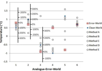
For level 1 assessment of large-scale features (i.e.c,landvin Eq. 1), a perfect algorithm would return the analogue-clean world features. Algorithms should, ideally, at least make the analogue-error worlds more similar to their analogue-clean worlds. Climatology, variability and long-term trends can be calculated for stations, regional averages or global averages from each adjusted analogue-error world. Similarity can be measured in terms of proximity in degrees Celsius for the cli-matology and linear-trend approximations and standard devi-ation as a measure of variability. This can be presented as per-centage recovery (after Williams et al., 2012). An example is shown in Fig. 2 for linear trend approximations with fur-ther explanation. Although linear trends do not describe the data perfectly, they provide a simple measure of long-term tendency that can be compared. This method does not indi-cate algorithms that result in a linear trend of the wrong sign (positive or negative). This may be seen as a more serious problem than a linear trend being over- or underestimated. Other scores, such as the squared error or the absolute error, could also be used to measure differences between adjusted analogue-error worlds and analogue-clean worlds.
Levels 2 and 3 are important for the developers of ho-mogenisation methods. They can be split into accuracy of change-point location detection and the accuracy of inhomo-geneity adjustments applied. In the case of gradual or season-ally varying inhomogeneities, the slope and seasonal cycle of
Figure 2.Example summary graph of algorithm skill for five hy-pothetical methods across six analogue-error worlds measured as trend-percentage recovery. This uses the trends calculated from an adjusted analogue-error world scaled against the difference be-tween the error world and its corresponding analogue-clean world. A 100 % trend recovery would indicate a perfect algo-rithm. Greater than 100 % would be moving the trend too far in the right direction. Less than 100 % would be an algorithm that does not move the trend far enough towards the analogue-clean world. A negative percentage would indicate an algorithm that moves the trend in the wrong direction. This method does not indicate algo-rithms that result in a trend of the wrong sign (positive or negative). This may be seen as a more serious problem than a trend being over-or underestimated and so would need to be identified separately.
the adjustments should also be assessed. Furthermore, a slid-ing scale may be used to penalise close but not exact hits rather than assigning them as misses. Care should be taken though considering that some algorithms may adjust the in-homogeneous data well, performing highly in the level 1 assessment, while not locating change points accurately or vice versa. For example, many small inhomogeneities may be homogenised by locating a single change point and ap-plying a single large amplitude inhomogeneity adjustment or vice versa. Similarly, a gradual inhomogeneity may be ho-mogenised by applying multiple small adjustments. Large inhomogeneities are easier to detect than small ones so as-sessment could be split into inhomogeneity size categories (e.g. Zhang et al., 2012). This information is of importance to algorithm developers.
Arguably, adjusting for detected inhomogeneities that are not actual inhomogeneities (false detection) adds error to the data and so could be scored more negatively than missing a real inhomogeneity. However, this critically depends upon the size of the adjustments applied. If adjustments for false detections are small there will be little change in climatol-ogy and trend statistics, hence the cost of false detection diminishes.
Table 2.Example contingency table for assessing change-point location detection and inhomogeneity adjustment skill (option shown in brackets) of homogenisation algorithms. Potential detections are the number of potential change points within the time period minus the total number of detections and misses. These are used to quantify those occasions where no change point is found and none is present. One way to do this is to assume that there is potentially a maximum of 1 change point every 6 months (some algorithms can only search for change points with 6 months of data on either side) such that a 26-year period will have 52 potential change points.
Change point No. change points present Totals
Change point detected Hits: False alarms: 8 (7)
within±3 months 5 (4) 3 (3)
(inhomogeneity adjustment with the correct sign (±) and within±1◦C)
Change point not detected Misses: Correct non-detections: 44 (45)
within±3 months 2 (3) 42 (42)
(inhomogeneity adjustment (potential detections) value with the incorrect
sign or not within±1◦C)
Totals 7 (7) 45 (45) 52 (52)
Heidke skill score 61 % (50 %)
Probability of detection hit rate 71 % (57 %)
False alarm rate 7 % (7 %)
of hits, misses, false alarms and “correct non-detections” are counted and used to construct various skill scores (Menne and Williams, 2005). Defining the number of “correct non-detections” is not straightforward, especially where a sliding scale is used to define a “hit”. A method for doing this needs to be investigated. Alternatively, measures that consider only hits, misses and false alarms may be used. The ideas used to assess detection skill can be adapted to investigate size-of-adjustment skill, as shown in red in Table 2. This could be visualised for each data product using a scatter plot where each analogue-error world result is positioned according to its hit rate and false alarm rate. Users can quickly see on which worlds that particular data product/algorithm scores highly (high hit rate and low false alarm rate), and which worlds are problematic. This can be used to infer applicabil-ity of data products for a specific use or intercomparison with data products created from different algorithms.
Level 4 assessment should help inform us which analogue-error world is most similar to reality (if any) in terms of de-tected change points for each algorithm. This is useful for two reasons. Firstly, assuming the error structure is realistic, it may help to tell us something about uncertainty due to in-homogeneities remaining in the data. Secondly, it helps to improve later versions of benchmarks in terms of developing realistic error models.
Levels 1 and 2 are of primary focus for assessing uncer-tainty and comparing data products. Level 3 is of more im-portance to algorithm developers than data-product users, in-forming where best to focus future algorithm improvements. Level 4 is mainly aimed at the working group. For the first benchmark cycle, assessment should focus on levels 1 and 2
to provide a quick response to the benchmark users. Ulti-mately, all worlds and results from the assessment will be made publicly available, ideally alongside any associated data products. This will allow for further bespoke assessment as required by interested analysts.
It is important that this process is made easy to encour-age participation. Ideally, all participants would submit a homogenised version of all stations in each analogue-error world. Additionally, a list should be provided of detected change points. Optionally, submission of information about the adjustments applied could also be encouraged (e.g. mag-nitude, slope/non-linear-trend function, and seasonal cycle). This would enable the assessment of all levels. However, it is more likely that different groups will select different sta-tions based on their desired end product. These may be lim-ited to long stations only or limlim-ited to specific regions. This could be problematic for contingency table assessment given the inherent tendency for false alarm rates/miss rates to grow with increasing numbers of test events (i.e. number of sta-tions). Some groups may wrap their homogenisation into a fully gridded product such that they are unable to provide in-dividual homogenised stations or a list of adjustments. This would prevent any level 2 and 3 assessment.
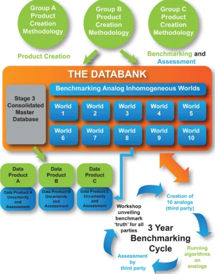
Figure 3.Schematic of the benchmarking assessment and benchmark cycle (source: Fig. 3 in Thorne et al., 2011).
participants could be asked to submit their best estimates of specified statistics such as the climatology, variance and linear trend. A set of regions could be specified such as the Giorgi regions commonly used within many aspects of cli-mate science (Giorgi and Francisco, 2000) in addition to hemispheric and global averages. A more accurate compar-ison could be done if groups submit lists of the stations in-cluded in gridded/regional products. It would also be pos-sible to specify a minimum subset of stations to be ho-mogenised to allow for a fair comparison across the region-ally focussed products, some of which may use manual ho-mogenisation methods and therefore unable to tackle global-scale homogenisation (cf. Venema et al., 2012). An important distinction could be made between best estimates of clean-world regional statistics and statistics calculated on all sta-tions within that region. In some cases it would be a wise decision to remove a station that has too many missing data or that is too poor in quality; however comparisons using all stations in the analogue-clean world compared to a partici-pant’s best estimate may penalise such approaches.
5 Providing a working cycle of benchmarking to serve the needs of science and policy
To ensure that homogenisation benchmarking achieves its full potential in terms of usefulness, the benchmarks need to be easily accessible and the assessment process timely with results that are easy to use. We envisage making the bench-mark worlds available alongside the ISTI databank in identi-cal format (Fig. 3) such that data-product creators can easily process them in addition to the real data.
If the cycle is too short then there are risks that not enough people will get involved, reducing the usefulness of product intercomparison. If the cycle is too long then the benchmarks become out of date and the assessment is too slow to be used alongside the CDR. Additionally, much may be learned about each analogue-error world from homogenising even without release of the underlying analogue-clean world. This runs the risk of second or third versions of algorithms becoming over-tuned to these specific worlds.
The wrap up would bring together users and creators of the benchmarks to assess how they were useful and how they can be improved for the next cycle. This will likely be in the form of a workshop and overview analysis paper. The databank will develop over time as will algorithms and the benchmarks will need to be updated both in terms of station coverage and methodologically.
The focus here is limited to monthly mean temperature data but it is envisaged that maximum and minimum temper-atures and, subsequently, daily temperature records will be included in the future. Also, the current framework is only set up to assess the homogenisation algorithm skill. There are many different aspects of data-product creation including quality-control processes, station selection and interpolation and gridding methods. The benchmarks created here could also be used to assess some of these, but at this time it was thought advantageous to focus only on the homogenisation element in order to make faster progress. We hope that the provision of this benchmarking framework will broaden in the future to include these other important aspects of data-product creation.
6 Concluding remarks
An international and comprehensive benchmarking system for homogenisation of global surface temperature data is es-sential for constraining the uncertainty in climate data arising from changes made to our observing system. The Interna-tional Surface Temperature Initiative is in a unique position to undertake this work and provide testing alongside the pro-vision of the raw climate data. A repeating cycle of bench-marking assessment has been proposed including concepts for creation of benchmark data and their assessment. The task is large and will take time to accomplish. However, this will for the first time enable global-scale quantification of uncer-tainty in station inhomogeneity, which is one of the least un-derstood areas of uncertainty associated with the land surface air temperature record.
The assessment of skill against the benchmarks will enable meaningful intercomparisons of surface temperature prod-ucts and assessment of fitness for purpose for a broad range of end users from large-scale climate monitoring to local-scale societal impacts analysis. Such a detailed and global testing of homogenisation algorithms will also be a signifi-cant aid to algorithm developers, hopefully resulting in vastly
improved algorithms for the future. These benchmarks can also be used to test other aspects of climate data record pro-duction such as station selection and interpolation. If suc-cessful, this work should significantly improve the robust-ness of monthly surface temperature climate data records on a range of spatial scales. This will improve the accuracy of assessment of recent changes in surface temperature and as-sociated uncertainties to end users.
Ultimately, the value of these benchmarks will only be as great as the number of groups participating in the exer-cise. The authors therefore strongly advocate development of new approaches and climate data records by new groups. The value of the new records will be greatly enhanced by under-taking benchmark testing as well as by using ISTI databank data.
Copyright statement
The works published in this journal are distributed under the Creative Commons Attribution 3.0 License. This license does not affect the Crown copyright work, which is re-usable under the Open Government Licence (OGL). The Creative Commons Attribution 3.0 License and the OGL are inter-operable and do not conflict with, reduce or limit each other.
©Crown copyright 2014
Acknowledgements. The work of Kate Willett was supported by the Joint UK DECC/Defra Met Office Hadley Centre Climate Programme (GA01101). Renate Auchmann was funded by the Swiss National Science Foundation (project TWIST). Constructive and comprehensive reviews by Blair Trewin, Richard Cornes and an anonymous reviewer served to improve the manuscript and are gratefully acknowledged.
Edited by: L. Eppelbaum
References
Aguilar, E., Auer, I., Brunet, M., Peterson, T. C., and Wieringa, J.: Guidelines on climate metadata and homogenization, WCDMP 53, WMO-TD 1186, World Meteorol. Organ., Geneva, Switzerland, 55 pp., 2003.
Auchmann, R. and Brönnimann, S.: A physics-based correction model for homogenizing sub-daily temperature series, J. Geo-phys. Res., 117, D17119, doi:10.1029/2012JD018067, 2012. Begert, M., Zenklusen, E., Häberli, C., Appenzeller, C., and Klok,
I.: An automated procedure to detect changepoints; performance assessment and application to a large European climate data set, Meteorol. Z., 17, 663–672, 2008.
Brockwell, P. J. and Davis, R. A.: Time Series: Theory and Meth-ods, 2nd Edn., Springer, New York, NY, 2006.
Brunet, M., Saladié, O., Jones, P. D., Sigró, J., Aguilar, E., Moberg, A., Lister, D., Walther, A., Lopez, D., and Almarza, C.: The development of a new dataset of Spanish daily adjusted tem-perature series (1850–2003), Int. J. Climatol., 26, 1777–1802, doi:10.1002/joc.1338, 2006.
Caussinus, H. and Lyazrhi, F.: Choosing a linear model with a ran-dom number of change-points and outliers, Ann. Inst. Statist. Math., 49, 761–775, 1997.
Caussinus, H. and Mestre, O.: Detection and correction of artificial shifts in climate series, J. Roy. Stat. Soc. Ser. C, 53, 405–425, 2004.
DeGaetano, A. T.: Attributes of several methods for detecting changepoints in mean temperature series, J. Climate, 19, 838– 853, 2006.
Domonkos, P., Poza, R., and Efthymiadis, D.: Newest developments of ACMANT, Adv. Sci. Res., 6, 7–11, doi:10.5194/asr-6-7-2011, 2011.
Ducré-Robitaille, J.-F., Vincent, L. A., and Boulet, G.: Comparison of techniques for detection of changepoints in temperature series, Int. J. Climatol., 23, 1087–1101, 2003.
Easterling, D. R. and Peterson, T. C.: The effect of artificial change-points on recent trends in minimum and maximum tempera-tures, International Minimax Workshop on Asymmetric Change of Daily Temperature Range, College Parg, MD, September 27– 30, 1993, Atmos. Res., 37, 19–26, 1995.
Giorgi, F. and Francisco, R.: Evaluating uncertainties in the predic-tion of regional climate change, Geophys. Res. Lett., 27, 1295– 1298, 2000.
Hannart, A. and Naveau, P.: An improved Bayes Information Crite-rion for multiple change-point models, Technometrics, 54, 256– 268, doi:10.1080/00401706.2012.694780, 2012.
Harrison, R. G.: Natural ventilation effects on temperatures within Stevenson screens, Q. J. Roy. Meteorol. Soc., 136, 253–259, doi:10.1002/qj.537, 2010.
Harrison, R. G.: Lag-time effects on a naturally ventilated large thermometer screen, Q. J. Roy. Meteorol. Soc., 137, 402–408, doi:10.1002/qj.745, 2011.
Karl, T. R., Williams Jr., C. N., Young, P. J., and Wendland, W. M.: A model to estimate the time of observation bias associated with monthly mean maximum, minimum, and mean temperature for the United States, J. Clim. Appl. Meteorol., 25, 145–160, 1986. Lawrimore, J. H., Menne, M. J., Gleason, B. E., Williams, C. N.,
Wuertz, D. B., Vose, R. S., and Rennie, J.: An overview of the Global Historical Climatology Network Monthly Mean Temper-ature Dataset, Version 3, J. Geophys. Res.-Atmos., 116, D19121, doi:10.1029/2011JD016187, 2011.
Lindau, R. and Venema, V. K. C.: On the multiple breakpoint prob-lem and the number of significant breaks in homogenisation of climate records. Idojaras, Q. J. Hung. Meteorol. Serv., 117, 1– 34, 2013.
Lu, Q., Lund, R. B., and Lee, T. C. M.: An MDL approach to the climate segmentation problem, Ann. Appl. Stat., 4, 299–319, doi:10.1214/09-AOAS289, 2010.
Menne, M. J. and Williams, C. N.: Detection of undocumented changepoints using multiple test statistics and composite refer-ence series, J. Climate, 18, 4271–4286, 2005.
Menne, M. J. and Williams Jr., C. N.: Homogenization of tempera-ture series via pairwise comparisons, J. Climate, 22, 1700–1717, 2009.
Menne, M. J., Williams Jr., C. N., and Vose, R. S.: The United States Historical Climatology Network monthly temperature data–Version 2, B. Am. Meteorol. Soc., 90, 993–1007, 2009. Parker, D. E.: Effects of changing exposure of thermometers at land
stations, Int. J. Climatol., 14, 1–31, 1994.
Peterson, T. C., Easterling, D. R., Karl, T. R., Groisman, P., Nicholls, N., Plummer, N., Torok, S. Auer, I., Boehm, R., Gullett, D., Vnicent, L., Heino, R., Tuomenvirta, H., Mestre, O., Szentim-rey, T., Salinger, S., Førland, E., Hanssen-Bauer, I., Hans Alexan-dersson, Jones, P., and Parker, D. E.: Homogeneity adjustments of in situ atmospheric climate data: A review, Int. J. Climatol., 18, 1493–1517, 1998.
Quayle, R. G., Easterling, D. R., Karl, T. R., and Hughes, P. Y.: Ef-fects of Recent Thermometer Changes in the Cooperative Station Network, B. Am. Meteorol. Soc., 72, 1718–1723, 1991. Reeves, J., Chen, J., Wang, Z. L., Lund, R., and Lu, Q.: A
Re-view and Comparison of Changepoint Detection Techniques for Climate Data. J. Appl. Meteor. Climatol., 46, 900–915, doi:10.1175/JAM2493.1, 2007.
Rennie, J. J., Lawrimore, J. H., Gleason, B. E., Thorne, P. W., Morice, C. P., Menne, M. J., Williams, C. N., de Almeida, W. G., Christy, J. R., Flannery, M., Ishihara, M., Kamiguchi, K., Klein-Tank, A. M. G., Mhanda, A., Lister, D. H., Razuvaev, V., Renom, M., Rusticucci, M., Tandy, J., Worley, S. J., Venema, V., Angel, W., Brunet, M., Dattore, B., Diamond, H., Lazzara, M. A., Le Blancq, F., Luterbacher, J., Mächel, H., Revadekar, J., Vose, R. S., and Yin, X.: The international surface tempera-ture initiative global land surface databank: monthly temperatempera-ture data release description and methods, Geoscience Data Journal, doi:10.1002/gdj3.8, online first, 2014.
Rohde, R., Muller, R. A., Jacobsen, R., Muller, E., Perlmutter, S., Rosenfeld, A., Wurtele, J., Groom, D., and Wickham, C.: A New Estimate of the Average Earth Surface Land Temperature Span-ning 1753 to 2011, Geoinfor Geostat: An Overview, 1, 7 pp., doi:10.4172/2327-4581.1000101, 2013.
Seneviratne, S. I., Nicholls, N., Easterling, D., Goodess, C. M., Kanae, S., Kossin, J., Luo, Y., Marengo, J., McInnes, K., Rahimi, M., Reichstein, M., Sorteberg, A., Vera, C., and Zhang, X.: Changes in climate extremes and their impacts on the natural physical environment, in: Managing the Risks of Extreme Events and Disasters to Advance Climate Change Adaptation, edited by: Field, C. B., Barros, V., Stocker, T. F., Qin, D., Dokken, D. J., Ebi, K. L., Mastrandrea, M. D., Mach, K. J., Plattner, G.-K., Allen, S. K., Tignor, M. and Midgley, P. M., A Special Report of Working Groups I and II of the Intergovernmental Panel on Cli-mate Change – IPCC, Cambridge University Press, Cambridge, UK, and New York, NY, USA, 109–230, 2012.
Titchner, H. A., Thorne, P. W., McCarthy, M. P., Tett, S. F. B., Haimberger, L., and Parker, D. E.: Critically Reassess-ing Tropospheric Temperature Trends from Radiosondes Us-ing Realistic Validation Experiments, J. Climate, 22, 465–485, doi:10.1175/2008JCLI2419.1, 2009.
Trewin, B.: Exposure, instrumentation, and observing practice ef-fects on land temperature measurements, WIREs Clim. Change, 1, 490–505, 2010.
Trewin, B.: A daily homogenized temperature data set for Australia, Int. J. Climatol., 33, 1510–1529, doi:10.1002/joc.3530, 2013. Venema, V., Bachner, S., Rust, H. W., and Simmer, C.:
Sta-tistical characteristics of surrogate data based on geophysi-cal measurements, Nonlin. Processes Geophys., 13, 449–466, doi:10.5194/npg-13-449-2006, 2006.
Venema, V. K. C., Mestre, O., Aguilar, E., Auer, I., Guijarro, J. A., Domonkos, P., Vertacnik, G., Szentimrey, T., Stepanek, P., Zahradnicek, P., Viarre, J., Müller-Westermeier, G., Lakatos, M., Williams, C. N., Menne, M. J., Lindau, R., Rasol, D., Rustemeier, E., Kolokythas, K., Marinova, T., Andresen, L., Acquaotta, F., Fratianni, S., Cheval, S., Klancar, M., Brunetti, M., Gruber, C., Prohom Duran, M., Likso, T., Esteban, P., and Brandsma, T.: Benchmarking homogenization algorithms for monthly data, Clim. Past, 8, 89–115, doi:10.5194/cp-8-89-2012, 2012. Vincent, L. A.: A technique for the identification of
inhomo-geneities in Canadian temperature series, J. Climate, 11, 1094– 1104, 1998.
Vincent, L. A., Wang, X. L., Milewska, E. J., Wan, H., Yang, F., and Swail, V.: A second generation of homogenized Canadian monthly surface air temperature for climate trend analysis, J. Geophys. Res., 117, D18110, doi:10.1029/2012JD017859, 2012.
Wang, X. L.: Accounting for autocorrelation in detecting mean-shifts in climate data series using the penalized maximal t or F test, J. Appl. Meteorol. Clim., 47, 2423–2444, doi:10.1175/2008JAMC1741.1, 2008a.
Wang, X. L.: Penalized maximalF test for detecting undocumented mean-shift without trend change, J. Atmos. Ocean. Tech., 25, 368–384, doi:10.1175/2007JTECHA982.1, 2008b.
Wang, X. L., Wen, Q. H., and Wu, Y.: Penalized MaximaltTest for Detecting Undocumented Mean Change in Climate Data Series, J. Appl. Meteorol. Clim., 46, 916–931, doi:10.1175/JAM2504.1, 2007.
Williams Jr., C. N., Menne, M. J., and Thorne, P.: Benchmark-ing the performance of pairwise homogenization of surface tem-peratures in the United States, J. Geophys. Res., 117, D05116, doi:10.1029/2011JD016761, 2012.
WMO: WMO No. 182, International meteorological vocabulary, Geneva, Switzerland, 1992.
WMO: Final Report, Commission for Basic Systems. Working Group on Data Processing, Task Group on WMO/CTBTO Mat-ters, 15–17 July 1998, www.wmo.int/pages/prog/www/reports/ wmo-ctbto.html, Geneva, Switzerland, 1998.
Xu, W., Li, Q., Wang, X. L., Yang, S., Cao, L., and Feng, Y.: Ho-mogenization of Chinese daily surface air temperatures and anal-ysis of trends in the extreme temperature indices, J. Geophys. Res.-Atmos., 118, 9708–9720, doi:10.1002/jgrd.50791, 2013. Zhang, J., Zheng, W., and Menne, M. J.: A Bayes factor model for