www.atmos-chem-phys.org/acp/3/941/
Chemistry
and Physics
Accounting for local meteorological effects in the ozone time-series
of Lovozero (Kola Peninsula)
O. A. Tarasova1and A. Yu. Karpetchko2∗
1Atmosphere Physics Department, Faculty of Physics, Moscow State University, Moscow, Russia 2Polar Geophysical Institute, Apatity, Russia
∗
Present address Finnish Meteorological Institute, Sodankyla, Finland
Received: 20 November 2002 – Published in Atmos. Chem. Phys. Discuss.: 10 February 2003 Revised: 30 June 2003 – Accepted: 2 July 2003 – Published: 7 July 2003
Abstract. The relationship between local meteorological conditions and the surface ozone variability was studied by means of statistical modeling, using ozone and meteorolog-ical parameters measured at Lovozero (250 m a.s.l., 68.5◦N, 35.0◦E, Kola Peninsula) for the period of 1999–2000. The re-gression model of daily mean ozone concentrations on such meteorological parameters as temperature, relative humidity and wind speed explains up to 70% of day-to-day ozone vari-ability in terms of meteorological condition changes, if the seasonal cycle is also considered. A regression model was created for separated time scales of the variables. Short-term, synoptical and seasonal components are separated by means of Kolmogorov-Zurbenko filtering. The synoptical scale variations were chosen as the most informative from the point of their mutual relation with meteorological param-eters. Almost 40% of surface ozone variations in time peri-ods of 11–60 days can be explained by the regression model on separated scales that is 30% more efficient than ozone residuals usage. Quantitative and qualitative estimations of the relations between surface ozone and meteorological pre-dictors let us preliminarily conclude that at the Lovozero site surface ozone variability is governed mainly by dynamical processes of various time scale rather than photochemistry, especially during the cold season.
1 Introduction
Surface ozone levels and its changes are of great interest since harmful effects of O3and positive trends of its concen-tration were established at a number of northern hemispheric locations (Scheel et al., 1997; Roemer, 2001). Since many processes are affecting the ozone concentrations, it is diffi-cult to isolate long-term ozone changes connected to changes Correspondence to: O. A. Tarasova
(Otarasova@yandex.ru)
in the chemical composition of the atmosphere from changes driven by meteorological processes of different time scales from global climate changes to local processes of ozone gen-eration and destruction in the frontal systems.
Chemical ozone generation and deposition on the surface are known to be strongly affected by meteorological con-ditions. For example, ozone levels tend to be higher un-der hot, sunny conditions favorable for photochemical ozone production in the presence of precursors. At the same time higher temperatures cause convection to develop, which in turn can enhance vertical ozone transport. Conversely, wet, rainy weather with high relative humidity is typically asso-ciated with the low ozone levels provided by less intensive photochemical production and, possibly, by ozone deposi-tion on water droplets (Lelieveld and Crutzen, 1990). Windy weather can influence ozone concentration near the surface in a different way. In particular, strong wind reflects the in-creased intensity of the vertical transport. If the boundary layer acts as a source of ozone due to chemical generation, the growth of the wind speed leads to the decrease of ozone concentration because of the vertical mixing. Conversely, if the ozone chemical budget in the boundary layer is negative, vertical transport transfers ozone-rich air from aloft down-ward, and surface ozone concentrations correlate positively with the wind speed.
30% of ozone variability, with highest ozone values associat-ing with ozone transport from industrial areas from south-west and losouth-west values associating with Artic air masses from North-East (Karpetchko et al., 2001).
Although the relationship between some meteorological parameters and surface ozone has been statistically estab-lished for some sites, both in urban and remote conditions (Bloomenfield et al., 1996; Dapeng Xu et. al., 1996, Gardner and Dorling, 2000), the physical background of the statisti-cal results is not completely understood yet. Among widely used statistical models the multilayer perception (MLP) neu-ral network, linear regression and regression tree can be men-tioned (Gardner and Dorling, 2000 and references therein). While MLP models are mostly used for the forecast aims and have low physical background, regression models are well defined in physical terms and allow the possibility to investi-gate impacting processes. The first attempt to use separated scales for modeling was made by Flaum et al. (1996), who used the separated seasonal component of ozone variations for a regression model creation on the basis of air tempera-ture and dew point temperatempera-ture dependence.
In this paper we present results of the investigation of me-teorological effects on the surface ozone time-series from the site located in the northwestern part of Russia. Both the re-gression analysis of the original deseasonalized data and sep-aration of the time scales were applied. Decomposition of the original data into the different time scale components iso-lates the periods which contribute mostly to the bulk corre-lation. This information is important for a better understand-ing of the processes underplayunderstand-ing the statistical relationships between surface ozone and meteorological parameters. The results presented here could also be of importance for the construction of a regression model of surface ozone varia-tions.
2 Measurements
The Lovozero site (250 m a.s.l., 68.5◦N , 35.0◦E) is located on the Kola Peninsula plateau on the bank of Lake Lovozero. The site was operating in the frames of European project TOR-2 (Tropospheric Ozone Research). Lovozero is sit-uated away from strong anthropogenic pollutant sources. Only a slight influence of the industrial towns of Apatity or Monchegorsk located at the distances of 80 km to the south-west or 120 km to the south-west, respectively, is possible. This influence is very small during the warm periods when north-ern and eastnorth-ern winds are prevailing. The Lovozero site is situated in the tundra region so VOC emission is also weak (Guenther et al, 1995; Guenther et al, 2000).
The climate of Kola Peninsula is specific in comparison with the other regions of Russia located at the same lat-itude due to its unique position between the Barents Sea with the hot Gulfstream and big continental areas at the south. The mean temperature for the period of
measure-ments was +0.9◦C. The coldest registered temperature was
−36.9◦C and the hottest one was +30.5◦C. During the year the coldest monthly temperatures was observed in January-February (−10◦–15◦C) while the hottest month was July (about +15◦C). Relative humidity all year round was about 75–90%. The site surrounding is under the stable snow cover from late October-early November till the beginning of May. Snow cover substantially reduces O3 surface depo-sition (Galbally and Roy, 1980). As a result, O3deposition differs strongly between summer and winter.
Prevailing wind directions at the site location are Northern (0 Degrees), South-Eastern (150 Degrees) and North-West-Western (285 Degrees).
The main features of the local meteorological conditions are determined by the site position north of the polar cycle so there polar day (June-mid July) and polar night (December-mid January) are clearly observed. The temperature inver-sions are quite rare during summer months and occur often in winter causing weaker ozone destruction near the ground in summer than in winter. As the natural and anthropogenic emissions are low, in situ ozone production in the area sur-rounding the site is low.
Measurements of the surface ozone concentration were carried out in Lovozero since January 1999 up to the present. For the measurements DASIBI 1008-AH analyzer with auto-matic temperature and pressure corrections was used. The in-strument was calibrated against the reference generator of the Laboratory of Ecological Control (St. Petersburg in 1998) and cross examined with DASIBI 1008-RS instrument. The calibration data was also verified by the similar instrument operating at the Russian ozone measuring network and by the instrument used in the international experiment TROICA (Crutzen et al., 1998). The sample uptake was 10 seconds, and the stored data resolution was 1 min, from which hourly, daily and monthly averages were calculated.
The standard meteorological parameters with the standard resolution of 3 hours were provided by Lovozero meteoro-logical station situated on the same Kola plateau. These include temperature, relative humidity, wind speed and di-rection, and precipitation. Wind direction data are avail-able only since May 2000, so they were not included in the analysis procedure. The meteorological data were provided by Russian Hydrometeorological Service and station itself is included in Russian governmental meteorological network which supports a high quality of meteorological data.
0 5 10 15 20 25 30 35 40 45 50 0,0
0,2 0,4 0,6 0,8 1,0
daily mean surface O
3, ppbv
norm
a
liz
ed his
to
g
ram
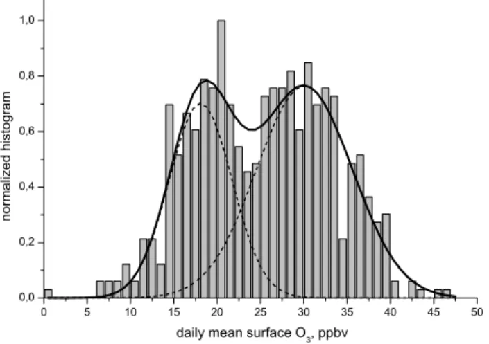
Fig. 1. Normalized histogram of daily mean surface ozone concen-trations at Lovozero site for the period 1999–2000 (the Gaussian approximating functions are presented by dot lines and their sum is solid line).
concentration distribution can be partly related to the local conditions like polar days and nights and inversions absence at Lovozero site. Nevertheless the shape of the histogram re-mains bi-modal if daily and night conditions are separated. The changes from one regime to another probably can be at-tributed to the snow coverage. Histograms of hourly mean concentrations for the subsets with and without snow cov-erage have only one peak. But it should be understood that “snow” subsets do not contain a full seasonal cycle. There is no clear explanation of the bi-modal structure yet and addi-tional study of this phenomenon is necessary.
The maximum hourly mean ozone value for the analyzed period was 59 ppbv and the minimal value was 9 ppbv. The mean value of the surface ozone concentration was 26 ±
9 ppbv for the period of 1999–2000. The principal feature of the seasonal variations of the surface ozone concentration at Lovozero site is the appearance of the spring maximum in April and minimum in August. The amplitude of the sea-sonal ozone variations was about 20 ppbv (in 1999) and com-parable with the northern Finland sites (Laurila, 1999). Sim-ilar seasonal ozone variations are observed at background European stations. In 2000 at Lovozero the secondary sea-sonal maximum was observed in summer and the amplitude of seasonal variations was only 12 ppbv. A possible expla-nation for the observed seasonal variations at the site could be stratosphere-troposphere exchange. Spatial transport fea-tures of year 2000 may cause conditions favorable for the secondary maximum formation but this phenomenon needs additional study.
Diurnal variations at the site are also typical for back-ground locations. The highest amplitude of the diurnal vari-ations is observed during the warm period of the year. Sur-face ozone concentration reaches its minimum values in the morning when ozone deposition on the surface under
temper-ature inversions plays an important role. Maximum ampli-tude of diurnal variations is registered in summer and reaches 10 ppbv.
3 Regression for daily mean ozone
In this chapter we present the results of the regression mod-eling of the surface ozone variations related to the variability of local meteorological parameters. We chose temperature, pressure, wind speed and relative humidity as proxies for the model as they are the only available meteorological parame-ters. Moreover they are the usual proxies for the regression models of the surface ozone (Bloomenfield et al., 1996; Roe-mer, 2001) and characterize main processes driven by local meteorology like in situ photochemical production, deposi-tion and vertical transport. Despite the fact that those param-eters are not completely independent, we will consider the variables to be complementary because they influence ozone through different processes. Surface pressure was also in-cluded in the model accounting for the synoptic scale ozone variations connected with the passages of the different syn-optic systems.
Like ozone there are some of the mentioned meteorologi-cal variables that have a strong seasonal cycle. Therefore the seasonal variations were removed from data series before the regression analysis. To describe the seasonal cycle the tech-nique proposed by Zvyagintsev et al. (1996) was used. The annual component was described as a sum of sine and cosine terms both with the period of 365.25 days. However, the sea-sonal behavior of ozone is not a pure monochromatic oscil-lation, so that the semiannual component was also included into the model fitting of the seasonal cycle. In the ozone case, the sum of the annual and the semiannual components accounts for about 50% of the total day-to-day variance of ozone. The correlation coefficients between deseasonalized ozone and the meteorological parameters are presented in Ta-ble 1.
Table 1. Correlation coefficients between the residuals of surface ozone and meteorological parameters
Correlation coefficients between surface ozone and...
temperature humidity pressure wind speed
Winter 0.48±0.08 0.17±0.10 −0.19±0.10 0.48±0.08 Spring 0.57±0.05 −0.25±0.07 −0.10±0.07 0.09±0.07 Summer 0.47±0.06 −0.17±0.07 0.09±0.08 0.19±0.07 Autumn −0.15±0.07 −0.38±0.07 0.07±0.08 0.52±0.06 Year 0.33±0.04 −0.22±0.04 −0.04±0.04 0.30±0.04
Table 2. Regression coefficients (with errors) and different mea-sures of regression models effectiveness (R2andd2) for the residu-als usage
Temperature Humidity Wind speed R2 d2
Winter 0.16±0.06 − 0.58±0.21 0.27 0.66 Spring 0.70±0.08 −0.14±0.04 − 0.38 0.72 Summer 0.64±0.09 − 0.92±0.30 0.25 0.63 Autumn −0.35±0.09 −0.13±0.05 1.50±0.20 0.37 0.72 Year 0.31±0.04 −0.13±0.02 0.51±0.10 0.17 0.55
correlation of ozone residuals with wind speed changes re-markably between autumn-winter and spring-summer peri-ods. In autumn-winter correlation coefficient is about 0.5, suggesting that ozone in the boundary layer has its origin in the free troposphere as there are no any significant sources of ozone near the ground. The small correlation coefficients in the spring-summer mean that vertical gradients of ozone are weak during this part of the year. The processes asso-ciated with the wind speed changes are strongly affected by the site’s position at the latitude where the vertical exchange is intensified in the Planetary Frontal Zone and tropopause folds happen quite often (Beekmann et al., 1997). The cor-relation coefficient of the ozone residuals with pressure is seen to be small all the year long. It implies, probably, that the origin of the synoptical systems is more significant than the systems themselves. For example, anticyclones coming to Kola Peninsula from the south differ strongly in ozone response from the arctic ones coming from the north (Kar-petchko et al., 2001). The separation of the ozone data set in accordance to the transport patterns may be necessary before surface pressure dependence can be established.
The stepwise method (which takes into consideration only the variables changing the total dispersion) for construction a multiple linear regression of the ozone concentration was used. The models were created for the complete data set and for different seasons separately. The results obtained are pre-sented in Table 2 and Fig. 2. It can be seen that the step-wise regression method did not include the pressure into any model as it does not improve the model quality.
0 20 40 60 80
10 15 20 25 30 35 40 45
50 spring, 1999 LOVOZERO
su
rf
ace
oz
one
,
ppb
v
days from the spring beginning
measurements yearly regression seasonal regression
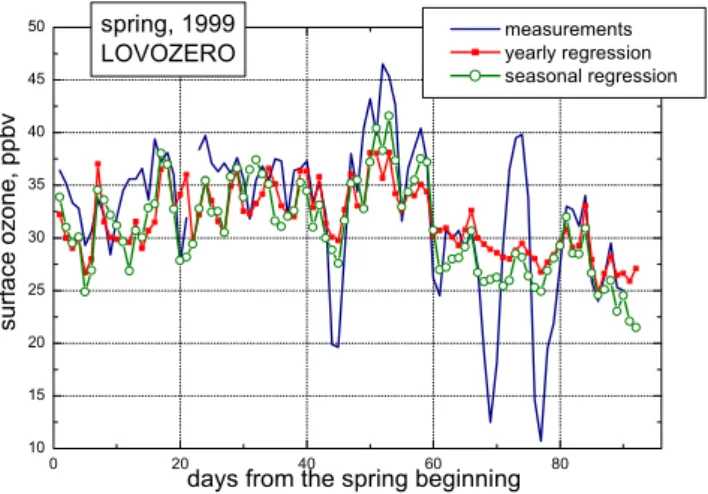
Fig. 2. Regression model of daily mean surface ozone on the local meteorological parameters (spring of 1999).
Two different measures of the effectiveness of the models are presented in the last two columns of Table 2. The first one is the determination coefficient (R2) which indicates how much of variability in the observed data is being reproduced by model. A more useful measure (Gardner and Dorling, 2000) of the model performance is provided by the “index of agreement” which is defined as
dα =1−
N
P
i=1
|Pi−Oi|α
N P
i=1
|Pi−O| + |Oi −O| α
(1)
wherePi andOi are modeled and observed concentrations. The index of agreement can be calculated for both α = 1 and 2. Both values ofdα are normalized and indicate the ex-tent that predicted deviations differ from the observed devia-tions about the mean observed value, indicating the degree to which model predictions are error free. Statisticsd2is more sensitive to the model quality than d1 since it is based on simple differences rather than squared differences..
The regression coefficients for the complete data set are presented at the bottom of the table. It can be seen that this model is not very effective because the determination coefficient reaches only 0.17. Such a low effectiveness of the model originates, probably, from the fact that processes governing the relations between ozone and meteorological parameters differ significantly during the year and can even change sign (see Table 1).
-0,4 -0,3 -0,2 -0,1 0,0 0,1 0,2 0,3 0,4 0,5
<1
1
11
-2
3
23
-3
5
35
-4
7
47
-5
8
58
-7
0
70
-8
2
82
-9
3
9
3-105
1
05-11
7
1
17-12
8
1
28-14
0
1
40-15
1
1
51-16
3
1
63-17
5
periods, days
c
o
rr
el
at
io
n
co
ef
fi
c
ient
temperature humidity pressure wind speed
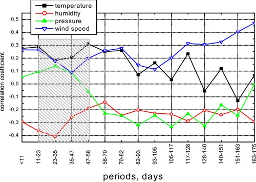
Fig. 3. Correlation coefficients for the separated scales of surface ozone and meteorological parameters variations (synoptical periods are shadowed).
withi=1 ...4 are different for each season. The resulting model can explain about 32% of the ozone variance. This shows that seasonal model is almost twice more effective than the model without consideration of the seasonal depen-dence of the regression coefficients. The higher effective-ness of the seasonal model may be explained by the changes of the prevailing meteorological processes which impact the surface ozone concentration for the different seasons. Taking into account the model of seasonal ozone cycle, the surface ozone concentrationCO3(d)can be expressed in the
follow-ing form: CO3(d)=CO+
X
i
[Aicos(2π d/T )+Bisin(2π d/T )]+ KT∗T (d)+KH∗H (d)+KW∗W (d)+R(d), (2) whereC0is a constant, the sum within parenthesis describes the seasonal cycle, which includes annual and semiannual components,KT,KH,KW are corresponding regression co-efficients with the residuals of temperatureT (d), humidity H (d)and wind speedW (d), andR(d)are ozone residuals after the regression on the meteorological parameters appli-cation, and d corresponds to the day of the year. This model explains about 70% of the total variance of the surface ozone concentration.
The results of two models with season-dependent and con-stant coefficients are presented in Fig. 2. To show the capa-bility of the models to capture day-to-day ozone variations, three months of the spring of 1999 are presented in the plot. It can be seen that the model with season-dependent coeffi-cients fits the observations better.
4 Time scales separation
It is of importance to estimate how the relations between sur-face ozone variations and meteorological parameters change on different time scales.
Time scale separation can be reached by the application of different filters (Randel, 1994; Marple, 1990). It was shown that the simplest way to reach a suitable degree of time scales separation is Kolmogorov-Zurbenko (KZ) filtering (Rao et al., 1997). Other filters can also be applied (Roemer and Tarasova, 2002), but they are not so efficient in the wide range of frequencies. Another advantage ofKZ method is its non-sensitivity to the gaps in the original data sets.
TheKZfilter is based on the running average calculation, applied to the time series several times. The output of the previous step serves as an input for the next step. Repeated application of the filter provides the necessary noise suppres-sion. The details of the filter characteristics can be found in Rao et al.(1997).
Table 3. “Signal/noise” ratio in the power spectrum of the separated components
Component ozone ln(O3) relative humidity temperature wind speed pressure
Seasonal 9.96 4.52 4.51 13.68 1.92 0.085
Synoptical 3.94 4.42 3.16 5.56 2.68 5.67
Short 2.43 2.92 4.46 1.95 5.01 1.58
the different periods ranges are presented in Fig. 3. The cor-relations at the longest possible periods present the “natural correlations” of the seasonal variations. Maximum correla-tion coefficients in the range of shorter periods are observed for humidity/ozone relations at the periods of 23–35 days, temperature/ozone relations at the periods of 47–58 days and wind speed/ozone relations at the periods of 11–23 days. So the most informative part of the spectrum from the point of the mutual correlations between surface ozone and meteoro-logical parameters lays in the range of the short periods be-tween 11 days and 2 months. This resulted in the following approach.
As the time series of the measurements is available only for 2 years, the following decomposition is applied:
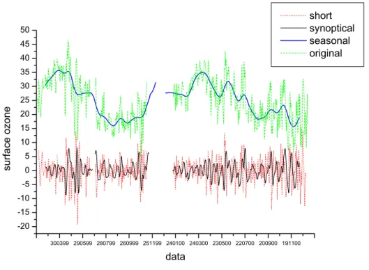
SH (t )=O3−KZ3,3(O3) (3) SY (t )=KZ3,3(O3)−KZ15,3(O3) (4) SE(t )=KZ15,3(O3) (5) whereSH (t )represents the short term component with the periods shorter than 11 days,SY (t )represents the synoptical scale variations from 11 days to 2 months, andSE(t ) repre-sents the seasonal component. As the daily mean values are used for the scales separation there are no diurnal variations included into the short term component.
The same decomposition is applied to the time series of the meteorological parameters: daily mean temperature, relative humidity, pressure and wind speed. The separated time series of surface ozone are presented in Fig. 4.
To evaluate the quality of separation the ratio of total power of useful/noise harmonics is estimated. The ratio shows the part of the energy in the selected range of peri-ods. The separation is quite poor for most of the compo-nents as it can be seen in Table 3. This is mainly due to the short length of the analyzed time series and short time resolu-tion, which causes strong aliasing and ringing effects in the analyzed spectra. Comparison of the separation of the log transformed ozone and non-transformed time-series shows that the seasonal component can be isolated better by use of the non-transformed ozone filtering, while for the other com-ponents the log transformation is preferable. Table 3 also demonstrates that the best separation of the seasonal compo-nent is obtained for the parameters with the strong seasonal behavior like ozone or temperature. Poor separation of the seasonal component is observed for pressure because of the small relative value of this type of variations.
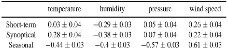
Table 4. Correlation coefficients between the separated time scales of surface ozone and meteorological parameters
correlation coefficients between surface ozone and...
temperature humidity pressure wind speed
Short-term 0.03±0.04 −0.29±0.03 0.05±0.04 0.26±0.04 Synoptical 0.28±0.04 −0.38±0.03 0.07±0.04 0.22±0.04 Seasonal −0.44±0.03 −0.4±0.03 −0.57±0.03 0.61±0.03
Table 5. Regression coefficients for synoptical component and model effectiveness
temperature humidity wind speed R2 d2
Winter − 0.10±0.09 1.19±0.27 0.48 0.84 Spring 0.63±0.07 −0.22±0.04 − 0.42 0.76 Summer 0.61±0.01 −0.11±0.04 0.22±0.30 0.36 0.72 Autumn −0.52±0.09 −0.12±0.07 1.92±0.26 0.45 0.78 Year 0.28±0.04 −0.21±0.03 0.44±0.12 0.22 0.59
5 Regression model for the synoptical component
The correlation coefficients between the separated compo-nents (Table 4) were compared with the ones obtained for the residuals in chapter 3. Obviously the highest correlations are observed between the seasonal courses of the separated com-ponents. Note that the correlations between ozone and tem-perature for the short and synoptical components are positive, and correlation coefficient is negative for the seasonal com-ponents. The correlation coefficients of the seasonal ozone component and meteorological parameters are substantially higher than for the annual residuals.
300399 290599 280799 260999 251199 240100 240300 230500 220700 200900 191100
-20 -15 -10 -5 0 5 10 15 20 25 30 35 40 45 50
s
ur
fac
e
o
z
on
e
data
short synoptical seasonal original
Fig. 4. Separation of the surface ozone time series.
210599 190899 171199 150200 150500 130800 111100 -10
-8 -6 -4 -2 0 2 4 6 8 10
ozo
ne s
y
no
ptic
al c
o
m
pone
nt,
pp
bv
Data
ozone (synoptical component) regression m odel
seasonal regression m odel
Fig. 5. Regression models application for the ozone synoptical component.
There is a very weak dependence of the synoptical scale ozone on temperature in winter and most of the variability is caused be the wind speed changes. This relationship is much stronger than in simple regression and the mechanism of this relation is described below. The dispersion is reduced nearly by a factor of two.
coefficient in the separated scales is larger and negative as well as in the simple regression model. This coefficient is statistically significant and very close in value for the sepa-rated scales and the simple regression model in summer and spring. Using the non-seasonal regression of synoptical scale ozone variations can explain 22% of the variability. Appli-cation of the seasonal regression shows that meteorological parameters can explain 42% of the synoptical scale variabil-ity of the surface ozone.
Comparison of the created regression models shows the following interesting features. The use of the separated scales is 30% more effective than application of the simple regression on the deseasonalized ozone time series. This is probably connected to the fact that the residuals contain not only the synoptical component, but also the short term one. It can be supposed that in the selected range of periods (11– 60 days) one of the most important mechanisms providing strong relation of the surface ozone variability with the mete-orological parameters is Rossby and longer Waves. This type of planetary waves was registered in total ozone (Khrgian and Kuznetsov, 1981). Planetary waves provide the changes of the vertical ozone gradient in the lower troposphere which may influence in the surface ozone variations. The spectral analysis of the synoptical components of ozone and meteo-rological parameters showed the main period of about 20– 25 days. These periods coincide with the Rossby and some other long waves periods. Relation of parameters in the re-gression model may be described by the following scheme: in the boundary layer of the atmosphere temperature rises adiabatically in descending air that is enriched with ozone and has low humidity during the wave passage. This way the air parcel reaches the surface with higher temperature, higher ozone concentration, higher wind speed and lower humidity. Additional study is necessary to confirm proposed mecha-nism.
6 Conclusions
In the paper the possibilities of the description of surface ozone variability in terms of the empiric regression models on the local meteorological parameters are discussed. Two different approaches to the regression models creation are compared. The first one is based on the usage of deseasonal-ized time series of the surface ozone concentration and local meteorological parameters for the regression modeling. The second approach is based on the separation of time scales by means ofKZfiltering technique with subsequent regression model creation for the selected time scale.
On the basis of the proposed methods some of the mech-anisms of the physical relations between surface ozone and meteorological predictors were clarified. Time scales sep-aration allowed to estimate the contribution of some mecha-nisms to the surface ozone variability and to find out the most effective periods of mutual correlations. Such an approach
gives the possibility to investigate the spatial and temporal structure of different processes contributing to the surface ozone variability.
The regression model of the ozone residuals after the sub-scription of the seasonal variations as parametric functions let us explain about 30% of the surface ozone variability on the basis of the local meteorological condition changes. The model including seasonal cycle can explain up to 70% of the surface ozone variability. At the same time it should be kept in mind that physical mechanisms driving the seasonal cycles of surface ozone and meteorological predictors can be differ-ent and this approach doesn’t demonstrate really physically grounded relations.
As a second approach the time scale separation was ap-plied. It was demonstrated that the highest correlation in the range of the short periods is observed between 11 days and 2 months. Three components separation for ozone and lo-cal meteorologilo-cal parameters (temperature, relative humid-ity, pressure and wind speed) was performed. The synoptical scale variations were chosen for the regression modeling as the most informative in the cross correlations of the surface ozone variations and local meteorological parameters.
The regression model of the synoptical scale ozone com-ponent on the meteorological parameters can explain about 40% of variability in terms of local meteorological condition changes of the same time scale. This model is 30% more efficient than the one on the basis of residuals since the re-lation between parameters is provided mainly by one sepa-rated process. This fact shows that at selected range of peri-ods about 40% of surface ozone variability at remote site is driven by the processes having similar responses to meteoro-logical variables.
Quantitative and qualitative estimations of the relation be-tween surface ozone and meteorological predictors let us preliminarily conclude that at least at a certain location (Lovozero site) surface ozone variability is governed mainly by dynamical processes of different time scales rather than photochemistry, especially during the cold season .
Acknowledgements. The work is carried out under the support of
Russian Foundation for Basic Research (grant N 00-05-64742, 02-05-64114, 03-05-64712) and INTAS (grant N 01-0016). The authors gratefully thank Hans-Eckhart Scheel (Forschungzentrum Karlsruhe, IMK-IFU, Germany) and Dr. Gennady I. Kuznetsov (Moscow State University) for the helpful comments during manuscript preparation and all the personnel working at the site for data acquisition (the laboratory of M.I. Beloglazov, Polar Geophys-ical Institute, Russia).
References
(Ecological Physics), Trukhin, V. I., Pirogov, Yu. A., Pokazeev, K. V. (Eds), Moscow, MAX Press, 9, 56–69, 2002.
Arabov, A. Yu., Elansky, N. F., Olshansky, D. I., Senik, I. A., Be-loglazov, M. I., Karpetchko, A. Yu., Kuznetsov, G. I., Tarasova, O. A., Kortunova, Z. V., Povolotskaya, N. P.: The temporal and spatial variations of surface ozone as observed at several sites of Russia, Atmospheric Ozone, Proceedings of the Quadrennial Ozone Symposium, HASDA, 679–680, 2000.
Beekmann, M., Ancellet, G., Blonsky, S., De Muer, D., Ebel, A., Elbern, H., Hendricks, J., Kowol, J., Mancier, C., Sladkovic, R., Smit, H. G. J., Speth, P., Trickl, T., and Van Haver, Ph.: Re-gional and global tropopause fold occurrence and related ozone flux across the tropopause, J.Atmos.Chem., 28, 29–44, 1997. Bloomenfield, P., Royle, J. A., Stainberg, L. J., and Qing, Y.:
Ac-counting for meteorological effects in measuring urban ozone levels and trends, Atm. Envir., 30 (17), 3067–3077,1996. Crutzen, P. J., Elansky, N. F., Hahn, M., Golitsyn, G. S.,
Bren-ninkmeijer, C. A. M., et al.: Trace gas measurements be-tween Moscow and Vladivostok using the Trans-Siberian rail-road, J.Atmos.Chem., 29, 179–194, 1998.
Elansky, N. F., Arabov, A. Ya., Senik, I. A., Kuznetsov, G. I., Tarasova, O. A., Beloglazov, M. I., Karpechko, A. Yu., Kor-tunova, Z. V.: The Features of Surface Ozone Variations in Re-mote, Rural and Urban Regions of Russia, TOR-2 Annual Report 2000, ISS, Munich Germany, 72–76, 2001.
Flaum, J. B., Rao, S. T., and Zubenko, I. G.: Moderating the influ-ence of Meteorological Conditions on Ambient Ozone Concen-trations, J. Air & Wast Manage.Assoc., 46, 35–46, 1996. Galbally, I. E. and Roy, C. R.: Destruction of ozone at the earth’s
surface, Q.J.R. Meteorol. Soc., 106, 599–620, 1980.
Gardner, M. W. and Dorling, S. R.: Statistical surface ozone mod-els: an improved methodology to account for non-linear be-haviour, Atmos. Envir., 34(1), 21–34, 2000.
Guenther, A., Geron, C., Pierce, T., Lamb, B., Harley, P., and Fall, R.: Natural emissions of non-methane volatile organic com-pounds, carbon monoxide, and oxides of nitrogen from North America, Atmos. Envir, 34 (12-14), 2205–2230, 2000.
Guenther, A., Hewitt, N., Erickson, D., Fall, R., Geron, C., Greadel, T., Harley, P., Klinger, T.,Lerdau, M., McKay, W., Pierce, T., Scholes, B., Streinbrecher, R., Tallamraju, R., Taylor, J., and Zimmerman, P.: A global model of natural volatile organic com-pounds emissions, J.Geophys.Res., 100, 8873–8892, 1995. Hogrefe, C., Rao, S., Xurbenko, I., and Porter, S.: Interpreting the
information in ozone observations and model predictions rele-vant to regulatory policies in the Eastern United States, Bulletin of the American Meteorological Society, 81, 2083–2106, 2000.
Karpetchko A. Yu., Elansky, N. F., Kuznetsov, G. I., Tarasova, O. A., Beloglazov, M. I., Rumyantsev, S. A.: The role of air transfer processes in the formation of surface ozone concentration fields over the Kola Peninsula, Izvestiya of Russian Academy of Sci-ence, Series Physics of the Atmosphere and Ocean, 37 (5), 692– 699, 2001.
Khrgian, A. H. and Kuznetsov, G. I.: The problem of atmospheric ozone observations and investigations, Moscow University Press, 216, 1981.
Laurila, T.: Observational study of transport and photochemical formation of ozone over northern Europe, J.Geophys.Res., 104 (D21), 26 235–26 243, 1999.
Lelieveld, J. and Crutzen, P. J.: Influence of cloud and photochem-ical processes on tropospheric ozone, Nature, 343, 227–233, 1990.
Marple Jr. S. R.: Digital spectral analysis with applications, Moscow, Mir, 584, 1990.
Roemer, M. and Tarasova, O.: Methane in The Netherlands – An ex-ploratory study to separate time scales, TNO report R 2002/215, The Netherlands, 2002.
Moody, J. L., Oltmans, S. J., Levy, II H., Merrill, J. T.: Trans-port climatology of tropospheric ozone: Bermuda, 1988–1991, J. Geophys. Res., 100 (D4), 7179–7194, 1995.
Randel, W. J.: Filtering and data processing for time series analysis, Methods of experimental physics, 28, 283–311, 1994.
Rao, S., Zurbenko, I., Neagu, R., Porter, S., Ku, J., and Henry, R.: Space and Time Scales in Ambient Ozone Data, Bulletin of the American Meteorological Society, 78, 2153–2166, 1997. Roemer, M.: Trends of ozone and related precursors in Europe,
Sta-tus report, TOR-2, Task group 1, TNO-report No. R-2001/244, 2001.
Scheel, H., Ancellet, G., Areskoug, H., et al.: Spatial and tem-poral variability of tropospheric ozone over Europe, In: Tropo-spheric ozone research: tropoTropo-spheric ozone in the regional and sub-regional context, Hov, Ø, Springer Verlag, Berlin, 35–45, 1997.
Tarasova, O. A., Elansky, N. F., Kuznetsov, G. I., Kuznetsova, I. N., Senik, I. A.: Impact of Air Transport on Seasonal Variations and Trends of Surface Ozone at Kislovodsk High Mountain Station, J. Atmos. Chem., (in press), 2003.
Xu, D., Yap, D., and Taylor, P. A.: Meteorologically adjusted ground level ozone trends in Ontario, Atm. Envir., 30 (7), 1117– 1124, 1996.