Using surface remote sensors to derive mixed-phase cloud radiative forcing: an example from M-PACE

(1)

ACPD

11, 12487–12518, 2011

Remotely-sensed cloud radiative

forcing

G. de Boer et al.

Title Page

Abstract Introduction

Conclusions References

Tables Figures

◭ ◮

Back Close

Full Screen / Esc

Printer-friendly Version Interactive Discussion

Discussion

P

a

per

|

Dis

cussion

P

a

per

|

Discussion

P

a

per

|

Discussio

n

P

a

per

|

Atmos. Chem. Phys. Discuss., 11, 12487–12518, 2011 www.atmos-chem-phys-discuss.net/11/12487/2011/ doi:10.5194/acpd-11-12487-2011

Atmospheric Chemistry and Physics Discussions

This discussion paper is/has been under review for the journal Atmospheric Chemistry and Physics (ACP). Please refer to the corresponding final paper in ACP if available.

Using surface remote sensors to derive

mixed-phase cloud radiative forcing:

an example from M-PACE

G. de Boer1, W. D. Collins1, S. Menon1, and C. N. Long2

1

Lawrence Berkeley National Laboratory, 1 Cyclotron Road, Berkeley, CA 94720, USA

2

Pacific Northwest National Laboratory, 902 Batelle Boulevard, Richland, WA 99352, USA Received: 21 March 2011 – Accepted: 14 April 2011 – Published: 20 April 2011

Correspondence to: G. de Boer (gdeboer@lbl.gov)

(2)

ACPD

11, 12487–12518, 2011

forcing

G. de Boer et al.

Title Page

Tables Figures

◭ ◮

Back Close

Full Screen / Esc

Discussion

P

a

per

|

Dis

cussion

P

a

per

|

Discussion

P

a

per

|

Discussio

n

P

a

per

|

Abstract

A suite of ground-based measurements are used in conjunction with a column version of the Rapid Radiative Transfer Model (RRTMG) to derive the cloud radiative forcing of mixed-phase stratiform clouds observed during the United States Department of Energy (US DOE) Atmospheric Radiation Measurement (ARM) Mixed-Phase Arctic 5

Clouds Experiment (M-PACE) between September and November of 2004. In total, sixteen half hour time periods are reviewed due to their coincidence with radiosonde launches. Cloud liquid (ice) water paths are found to range between 11.0–366.4 (0.5– 114.1) gm−2, and cloud physical thicknesses fall between 286–2075 m. Combined with temperature and hydrometeor size estimates, this information is used to calculate sur-10

face radiative fluxes using RRTMG, which are demonstrated to generally agree with measured fluxes from surface-based radiometric instrumentation. Errors in longwave flux estimates are found to be largest for thin clouds, while shortwave flux errors are generally largest for thicker clouds. Cloud radiative forcing is calculated for all profiles, and illustrates the dominance of the longwave component during this time of year, with 15

net cloud forcing generally between 50 and 90 Wm−2. Finally, sensitivity of calculated surface fluxes to droplet e_ffective radius, surface albedo and surface temperature are tested, with changes in minimum droplet size between 3.5 and 10 µm altering the sur-face shortwave flux by up to 50 Wm−2, and changes in surface albedo between 0.5 and 0.95 altering surface shortwave fluxes by up to 85 Wm−2.

20

1 Introduction

The radiative impacts of clouds remain one of the largest uncertainties in the simulation and understanding of global climate change (IPCC, 2007). In particular, clouds occur-ring in the Arctic have a potentially large impact on characteristics and lifetime of sea ice (e.g. Kay and Gettelman, 2009), permafrost, and plant growth (e.g. Prowse et al., 25

(3)

ACPD

11, 12487–12518, 2011

forcing

G. de Boer et al.

Title Page

Tables Figures

◭ ◮

Back Close

Full Screen / Esc

Discussion

P

a

per

|

Dis

cussion

P

a

per

|

Discussion

P

a

per

|

Discussio

n

P

a

per

|

both ice and liquid hydrometeors, are among the most-commonly observed, longest lasting and radiatively influential cloud structures (e.g. Curry et al., 1996; Shupe et al., 2006). As discussed in Shupe et al. (2008), observation of these clouds is inherently difficult due to the need to capture multiple phases of liquid simultaneously.

Despite these challenges, several previous efforts have provided estimates of Arctic 5

stratiform cloud radiative characteristics and forcing. While obtaining this estimate is not the central goal of the present study, we do provide an overview of these stud-ies and their methodologstud-ies for reference. Pioneering estimates of infrared radiative characteristics of summertime stratiform clouds over the Beaufort Sea were provided by Curry and Herman (1985) using a combination of radiometers, in-situ measure-10

ments and a radiative transfer model. In that work, cloud emittances, absorption co-efficients, reflectances, cooling rates and extinction lengths were reported. All param-eters were found to be strongly tied to liquid cloud droplet size distributions assumed and cloud liquid water path. Expanding on this work, Curry and Ebert (1992) utilized measurement-based estimates of cloud fraction and microphysical properties, along 15

with top of the atmosphere (TOA) radiative fluxes from the NASA Earth Radiation Bud-get Experiment (ERBE; Barkstrom et al., 1990) to calculate an annual cycle of radiative fluxes for different cloud types. Included were “low clouds” which were parameterized to have mean seasonal liquid water paths between 10–40 gm−2 and ice water paths between 0–60 gm−2. These estimates also included wintertime ice crystal precipitation 20

not associated with mixed-phase clouds. As in earlier work, the uncertainty associated with estimating cloud droplet effective radius was mentioned to be considerable. Net surface cloud forcing was demonstrated to be positive throughout most of the year, with any negative values occurring during the summer months, when cloud-induced shortwave cooling is slightly stronger than longwave heating.

25

(4)

ACPD

11, 12487–12518, 2011

forcing

G. de Boer et al.

Title Page

Tables Figures

◭ ◮

Back Close

Full Screen / Esc

Discussion

P

a

per

|

Dis

cussion

P

a

per

|

Discussion

P

a

per

|

Discussio

n

P

a

per

|

fluxes and those observed. Comparison of model calculations with clear-sky calcula-tions demonstrated a longwave cloud radiative forcing of up to 70 Wm−2. Shupe and Intrieri (2004) provide cloud radiative forcing calculations for an annual cycle of clouds observed during the Surface Heat Budget of the Arctic (SHEBA; Uttal et al., 2002), analyzing individual contributions of cloud properties on long and shortwave forcing for 5

observed clouds. They found that clouds with significant longwave impacts were gener-ally low clouds with warmer base temperatures, with longwave cloud forcing impacted strongly by liquid water path (LWP). Except during mid-summer, they found that long-wave effects dominate up to LWP values of 400 gm−2. They also demonstrated that for clouds containing liquid water, the longwave forcing dominates net cloud forcing on an 10

annual scale, resulting in a peak in the annual distribution of net cloud radiative forcing of approximately 50 Wm−2. An annual distribution of longwave cloud forcing for liquid-containing clouds was found to peak at 50–70 Wm−2. Summer cloud radiative forcing was also evaluated by Dong and Mace (2003). Utilizing surface remote sensors at Barrow for May–September, they found the net radiative forcing by stratus clouds to 15

become negative starting in late May, and stay negative until early September. The forcing was found to peak during June and July, with values up to−150 Wm−2. Stra-tus cloud longwave radiative forcing was found to range between roughly 40–70 Wm−2 during that time period.

In the current e_ffort, we utilize modern measurement and retrieval methods from 20

a combination of ground-based remote sensors used during the Mixed-Phase Arctic Cloud Experiment (M-PACE; Verlinde et al., 2007) to estimate the radiative forcing of mixed-phase clouds observed during this campaign. While surface radiative measure-ments are available for this time period, our main focus is characterizing the ability of a combination remotely-sensed measurements and a column version of the advanced 25

(5)

ACPD

11, 12487–12518, 2011

forcing

G. de Boer et al.

Title Page

Tables Figures

◭ ◮

Back Close

Full Screen / Esc

Discussion

P

a

per

|

Dis

cussion

P

a

per

|

Discussion

P

a

per

|

Discussio

n

P

a

per

|

perform experiments analyzing the method’s sensitivity to less frequently measured quantities such as cloud liquid e_ffective radius, surface temperature and surface albedo. An overview of methods and tools utilized is provided in the following section. This is followed by an overview of M-PACE clouds studied, an analysis of derived surface flux estimates and cloud radiative forcing and sensitivity experiments. Finally, discussion 5

and a summary are provided.

2 Measurement period and methods

M-PACE was a United States Department of Energy (DOE) Atmospheric Radiation Measurement (ARM) experiment carried out along the north slope of Alaska (NSA) during the fall of 2004 aimed at collecting a focused set of observations to understand 10

Arctic mixed-phase clouds. Measurements used in this evaluation were collected at Barrow (71.3◦N, 156.6◦W). Because of the methods involved, it is necessary to take observations occurring close to a radiosonde launch time. With this restriction 16 cases featuring single-layer mixed-phase stratiform clouds were identified, covering a wide variety of cloud thicknesses, as well as liquid and ice water paths for both day and 15

nighttime periods (see Table 1). 2.1 Instruments and retrievals

To derive cloud properties, we utilized a combination of ground based remote sensors and information from launched radiosondes. The microphysical retrieval techniques implemented are similar to those described in de Boer et al. (2009), using the University 20

of Wisconsin Arctic High Spectral Resolution Lidar (AHSRL; Eloranta, 2005), a 35-GHz Millimeter Cloud Radar (MMCR; Moran et al., 1998) and microwave radiometer (MWR). Our focus on mixed-phase stratiform clouds is due in part to the challenge they present to microphysical retrieval algorithms. Retrievals implemented generally represent state-of-the-science attempts, as recommended in Shupe et al. (2008), and 25

(6)

ACPD

11, 12487–12518, 2011

forcing

G. de Boer et al.

Title Page

Tables Figures

◭ ◮

Back Close

Full Screen / Esc

Discussion

P

a

per

|

Dis

cussion

P

a

per

|

Discussion

P

a

per

|

Discussio

n

P

a

per

|

To begin, cloud boundaries are determined using the cloud radar and lidar. A combi-nation of AHSRL backscatter cross-section and depolarization is used to find the base of the liquid component of the cloud (Zbase). All ice found below that is assumed to be

precipitation. Because the lidar signal is often completely attenuated within the cloud layer, MMCR reflectivity is used to find cloud top (Z_top). It is important to note that due 5

to near-field limitations of the radar, observations below 200 m are not included in any of the analysis presented.

Ice water content (IWC) is calculated using an empirical relationship from radar re-flectivity (Zmmcr) as prescribed in Shupe et al. (2006). The relationship used is:

IWC=0.07Z0_mmcr.63 (1)

10

While this equation is empirical, and tuned to a specific region, it is generally the best option available, since multi-sensor retrievals are limited by attenuation of the lidar and a liquid-dominated lidar backscatter signal.

Because the liquid cloud can not necessarily be detected by the radar, and atten-uation hinders lidar measurements, liquid water content (LWC) is calculated using a 15

scaled-adiabatic assumption (Zuidema et al., 2005). Utilizing temperature information from the radiosonde, the pseudo-adiabatic lapse rate (Γs) for a cloud is calculated.

From this, we calculate liquid water mixing ratio (wl) via integration of:

d wl=

cp

L_{l ,v}

Γs+

g cp

d z (2)

with c_p being the specific heat of air at a constant pressure, L_{l ,v} the latent heat of 20

vaporization,z the altitude, and gthe acceleration due to gravity. Multiplication of the liquid water mixing ratio by the air density results in an estimate of LWC. Since these clouds are not necessarily adiabatic, we scale the calculated profile using the LWP derived from MWR measurements. Because this method depends on accurate tem-perature measurements, we can only calculate these properties close to radiosonde 25

(7)

ACPD

11, 12487–12518, 2011

forcing

G. de Boer et al.

Title Page

Tables Figures

◭ ◮

Back Close

Full Screen / Esc

Discussion

P

a

per

|

Dis

cussion

P

a

per

|

Discussion

P

a

per

|

Discussio

n

P

a

per

|

Ice and liquid hydrometeor effective sizes are more challenging to derive. For the ice e_ffective particle size (re,ice), we utilize a multi-instrument retrieval (AHSRL and

MMCR) as described in Donovan and van Lammeren (2001), using the ratio of the lidar and radar backscatter to estimate particle effective size. This can only be done below the liquid portion of the cloud due to dominance of the lidar signal by the liquid 5

component of the mixed-phase cloud. Therefore, once inside the cloud layer, we utilize a scaling factor calculated just below cloud base based on the ratio of radar reflectivity just below cloud base to radar reflectivity throughout the cloud. This ratio is raised to the 1/6th power, since radar backscatter cross section is proportional tor6. Values of

re,ice within the cloud layer are then calculated using this scaling factor and the below

10

cloudr_e,_ice. Liquid droplet e_ffective radius (r_e,_liq) is not constrained, since we can not observe the depth of the liquid component of the cloud. Therefore, calculate a profile ofre,liq that assumes an initial cloud-base droplet size, and scales to the LWC profile,

assuming a constant droplet number concentration calculated using this cloud-base droplet size and LWC.

15

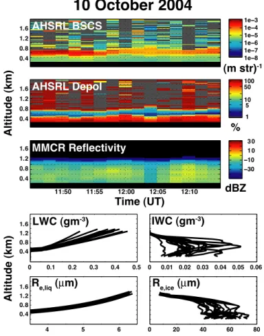
An example of the measurements and retrievals is provided in Fig. 1. Included in the top half of Fig. 1 are plots of the AHSRL-measured backscatter cross-section (β′, top) and depolarization (δ, middle), as well as MMCR reflectivity (Zmmcr, bottom). The data

have been averaged to 2-minute intervals in order to reduce noise and variability in the information passed into the radiative transfer model. Higher values ofβ′observed 20

at roughly 500–800 m are the result of liquid droplets. Because of the concentration of these droplets they have a large combined backscatter cross-section. The AHSRL

δ is used to help determine cloud phase, with lower depolarization ratios generally resulting from spherical scatterers. Due to the thickness of the liquid portion of this cloud, the lidar signal is attenuated before reaching cloud top. This is seen in Zmmcr,

25

(8)

ACPD

11, 12487–12518, 2011

forcing

G. de Boer et al.

Title Page

Tables Figures

◭ ◮

Back Close

Full Screen / Esc

Discussion

P

a

per

|

Dis

cussion

P

a

per

|

Discussion

P

a

per

|

Discussio

n

P

a

per

|

et al., 2008; McFarquhar et al., 2007), and that radar is capable of detecting cloud top altitude.

The lower half of Fig. 1 illustrates profiles of retrieved liquid and ice water content, as well as liquid and ice particle sizes for the 10 October case. These provide some perspective on the variability between individual profiles within a case. Because of the 5

pseudo-adiabatic assumption applied to the liquid portion of the cloud, liquid properties vary relatively linearly with altitude. Ice properties demonstrate more variability with altitude.

2.1.1 RRTMG

RRTMG is a global climate model version of the rapid radiative transfer model (RRTM). 10

It calculates long and shortwave fluxes utilizing a correlated-k method for computational e_fficiency. It has been demonstrated to be accurate when compared to line-by-line ra-diative calculations. Parts of RRTM are currently implemented in the European Center for Medium-Range Weather Forecasts (ECMWF) and National Centers for Environ-mental Prediction (NCEP) Global Forecast System (GFS) models, as well as the latest 15

version of the National Center for Atmospheric Research (NCAR) Community Climate System Model (CCSM4) as part of the Community Atmosphere Model (CAM). In this work, retrieved profiles of LWC, IWC,r_e,_ice, andr_e,_liq, solar zenith angle, surface tem-perature and albedo are used to drive a column version of RRTMG. Solar zenith angle is calculated for each given date and time, along with the earth’s radius at Barrow’s 20

(9)

ACPD

11, 12487–12518, 2011

forcing

G. de Boer et al.

Title Page

Tables Figures

◭ ◮

Back Close

Full Screen / Esc

Discussion

P

a

per

|

Dis

cussion

P

a

per

|

Discussion

P

a

per

|

Discussio

n

P

a

per

|

3 Analysis

3.1 Derived cloud properties

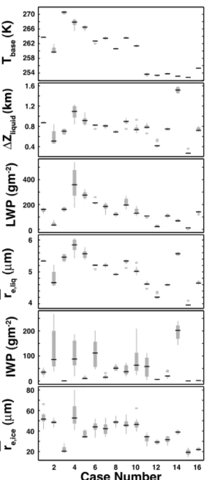
Although only a small sample, clouds observed close to radiosonde launches during M-PACE cover a variety of mixed-phase stratiform conditions. Estimates of mean cloud thickness (∆Zliquid), mean cloud liquid water path (LWP) and mean cloud ice water path

5

(IWP) are provided in Table 1 for each of the 16 cases analyzed. Figure 2 provides ad-ditional insight into the variability between and within cases. For each quantity, boxplots are laid out with the black line representing the mean, the shaded box representing the interquartile range (IQR) and whiskers representing the 10th and 90th percentiles for measured profiles within each case. Outliers (points outside of the 10th/90th percentile) 10

are represented by open circles. It is important to note that 2-min averaging results in only 6–15 profiles per case (depending on instrument calibrations and uptime), mean-ing small sample sizes for the distributions shown. Cloud base temperature for these cases was found to vary between 253–272 K. Due to the stratiform nature of the clouds, temperature generally did not vary very much within each case. Cases 11–16, occur-15

ring later in the year (end of October, beginning of November) had the coldest recorded temperatures.

The thickness of the liquid portion of the cloud varied between 300 and 1600 m, and within case 2, varied up to 400 m. Generally, clouds were found to be around 800 m thick. Retrieved liquid water paths also varied substantially between cases, ranging 20

from roughly 20 gm−2to over 500 gm−2. With the exception of cases 12 and 15, these clouds contained enough liquid (in a mean sense) to emit as grey bodies. The LWP threshold for this was demonstrated to be around 30 gm−2by Shupe and Intrieri (2004), with further increases in LWP having no impact on downwelling longwave radiation.

As discussed above, liquid droplet effective radii were constrained by measured liq-25

(10)

ACPD

11, 12487–12518, 2011

forcing

G. de Boer et al.

Title Page

Tables Figures

◭ ◮

Back Close

Full Screen / Esc

Discussion

P

a

per

|

Dis

cussion

P

a

per

|

Discussion

P

a

per

|

Discussio

n

P

a

per

|

to scale with cloud physical depth. Using this initial value, re,liq ranged from roughly

4–5.8 µm.

Ice water paths were found to vary quite widely, both between cases and within indi-vidual cases. Across the dataset, values varied between roughly 5–260 gm−2, though with the exception of case 14, case mean values did not exceed 125 gm−2. Mean 5

ice particle effective radii (re,ice) were estimated to fall between 15–80 µm. Generally,

variability for any individual case was small (with exception of case number 4), and

r_e,_ice generally fell between 30 and 50 µm. While the ice component of these clouds has been demonstrated to be less influential than the liquid phase at both visible and infrared wavelengths, it is not negligible.

10

3.2 RRTMG derived fluxes and cloud radiative forcing

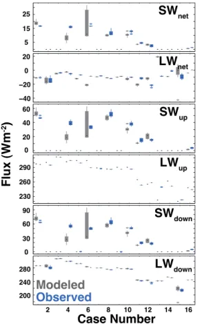
Initial analysis is completed on all 16 cases, assuming cloud-base r_e,_liq of 3.5 µm. Surface albedos for each case were calculated from surface radiometric data, with case-mean values ranging between 0.67 and 0.86. Finally, ground temperature was obtained from the National Oceanographic and Atmospheric Administration’s (NOAA) 15

US Climate Reference Network station at Barrow, which uses a Apogee Instruments IRTS-P infrared (IR) temperature sensor mounted on a tower at 1.3 m above ground level. Comparisons are completed using QCRAD, a quality-controlled surface radiation estimate product available through the ARM program database (Long and Shi, 2008). Results of this comparison are shown in Fig. 3. Shortwave (wavenumbers between 820 20

and 50 000 cm−1) and longwave (wavenumbers between 10 and 3250 cm−1) fluxes are shown, and broken down into surface downwelling, upwelling and net components. Each case features two distributions, with boxplots plotted identically to Fig. 2. Outly-ing values (values outside of the 10th/90th percentiles) are shown by open circles. The sign convention used results in positive net values at the surface when downwelling 25

flux is larger than upwelling flux.

(11)

ACPD

11, 12487–12518, 2011

forcing

G. de Boer et al.

Title Page

Tables Figures

◭ ◮

Back Close

Full Screen / Esc

Discussion

P

a

per

|

Dis

cussion

P

a

per

|

Discussion

P

a

per

|

Discussio

n

P

a

per

|

General patterns observed were replicated in the modeled data. The best agree-ment was found for downwelling longwave radiation, with a root-mean-squared error (RMSE) of 4.42 Wm−2. The upwelling longwave estimates had larger errors (RMSE of 9.19 Wm−2), likely due to errors in the surface temperature estimates used. Com-bined, these result in RMSE of 9.83 in the net surface longwave fluxes. For all of these 5

quantities, it should be noted that the majority of the error seems to come from a small subset of the cases, with cases 11, 13 and 14 having the largest differences between modeled and observed surface fluxes. As is shown in Fig. 2, these cases feature some of the smallest LWP observed. Shortwave errors were generally larger. RMSEs for downwelling, upwelling and net shortwave radiation were 10.01, 7.19 and 2.95 Wm−2 10

respectively. These numbers are muted due to contributions from nighttime cases, where both modeled and observed fluxes were zero. Removing nighttime cases, these values were increased to 13.96, 9.75 and 4.28 Wm−2.

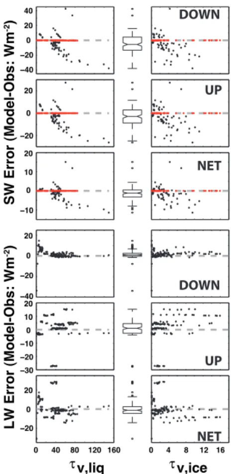
Error magnitude was also plotted against visible optical depth for each case (Fig. 4). The optical depths were computed separately for the liquid and ice components using 15

relationships from Stephens (1994) and Ebert and Curry (1992), respectively. The relationship for liquid is:

τ_vis_,_liq≈ 3LWP 2ρlre,liq

(3)

whereτvis,liq is the visible optical depth for liquid, LWP is the liquid water path,ρl is the

density of water, andr_e,_liqis the droplet effective radius. For ice, the relationship is: 20

τ_vis_,_ice≈IWP

a₊ b

re,ice

(4)

whereτ_vis_,_ice is the visible optical depth for ice, IWP is the ice water path, r_e,_ice is the ice crystal effective size, and a and b are wavelength-dependent parameters (avail-able in Ebert and Curry (1992), for visible wavelengths a=3.448×10−3m2g−1 and

(12)

ACPD

11, 12487–12518, 2011

forcing

G. de Boer et al.

Title Page

Tables Figures

◭ ◮

Back Close

Full Screen / Esc

Discussion

P

a

per

|

Dis

cussion

P

a

per

|

Discussion

P

a

per

|

Discussio

n

P

a

per

|

For shortwave fluxes illustrated in Fig. 4, it appears that errors in both up- and down-welling fluxes increase with increasingτvisfor both liquid and ice. Generally, shortwave

fluxes appear to be underestimated by the technique used. The cluster of cases that demonstrate zero error are the result of dark or very low-light cases, with nighttime cases (solar zenith angle≥90◦) illustrated in red. Errors in up- and downwelling com-5

ponents look very similar to one another due to the upwelling component simply being proportional to the downwelling by the albedo. It also appears as though clouds with lower LWP provide more di_fficulties for the model than thicker clouds, and that clouds with lowτvis,iceare the only ones that over predict the incoming (and therefore outgoing)

shortwave radiation. Net shortwave flux errors are generally less than 10 Wm−2. 10

For longwave fluxes, again the errors in net surface radiative flux are relatively small (generally<10 Wm−2). Downwelling longwave fluxes seem to be over-predicted, with errors<3 Wm−2 for cases with larger τ_vis_,_liq. Cases with smaller τ_vis_,_liq have errors up to roughly 10 Wm−2. The center column of Fig. 4 illustrates boxplots (similarly laid out to Fig. 2) illustrating the distribution of errors for each flux component. For shortwave 15

fluxes, nighttime errors were not included in these boxplots. Mean error values are presented in Table 2.

Cloud radiative forcing is calculated in a method similar to that used in Ramanathan et al. (1989). Here the short and longwave radiative forcing are defined as:

CFLW=F(Ac)−F(0) (5)

20

CFSW=Q(Ac)−Q(0) (6)

CF₌CF_LW₊CF_SW (7)

whereA_c is the cloud fraction, F and Q the net surface long- and shortwave fluxes, respectively, and theF(0) andQ(0) terms represent the clear-sky flux only. As in the rest of the paper, all fluxes are defined as positive downward. In order to determine the 25

(13)

ACPD

11, 12487–12518, 2011

forcing

G. de Boer et al.

Title Page

Tables Figures

◭ ◮

Back Close

Full Screen / Esc

Discussion

P

a

per

|

Dis

cussion

P

a

per

|

Discussion

P

a

per

|

Discussio

n

P

a

per

|

the temperature profile to remove inversions caused by cloud-top cooling. This was done via interpolation from the surface to the top of the cloud-induced inversion, creat-ing a linear temperature profile for that portion of the atmosphere.

Cloud radiative forcing estimates from this calculation are presented in Fig. 5. Dis-tributions of shortwave, longwave, and net cloud radiative forcing are provided for the 5

151 retrieved profiles. The contribution of nighttime and low light cases is evident in the large peak in shortwave forcing centered on 0 Wm−2. The rest of the cases are distributed on the negative side between 0 and −50 Wm−2 (cloud results in re-duced shortwave surface flux) due to variability in cloud properties and solar zenith angle. Longwave radiative forcing is positive, with a large peak around 75–85 Wm−2. 10

Both longwave and shortwave distributions are qualitatively similar to those collected by Shupe and Intrieri (2004) for a year of measurements from the SHEBA campaign. However, longwave cloud radiative forcing values are slightly higher (70–90 Wm−2 com-pared to 25–75 Wm−2) when compared to the Shupe and Intrieri (2004) study. This is likely due to the short time period covered in the current study, and the likely inclusion of 15

numerous thin liquid clouds in the one-year SHEBA dataset. The longwave values are higher but comparable to those reported by Dong and Mace (2003) for summer months in Barrow (40–70 Wm−2). Short- and longwave cloud radiative forcing estimates for Barrow during October from Dong et al. (2010) were smaller in magnitude than those derived in the current study, but their analysis was not limited to mixed-phase clouds or 20

liquid-containing clouds. Combined, the short- and longwave contributions result in a positive cloud radiative forcing for mixed-phase stratiform clouds observed during the M-PACE campaign. Net values range between roughly 25 and 90 Wm−2, with a ma-jority of cases falling in the 70–90 Wm−2 range. This means that mixed-phase clouds increase incoming radiation at the surface due to the longwave contributions during 25

the observed autumn period. An overview of mean cloud radiative forcing estimates is provided in Table 3.

(14)

ACPD

11, 12487–12518, 2011

forcing

G. de Boer et al.

Title Page

Tables Figures

◭ ◮

Back Close

Full Screen / Esc

Discussion

P

a

per

|

Dis

cussion

P

a

per

|

Discussion

P

a

per

|

Discussio

n

P

a

per

|

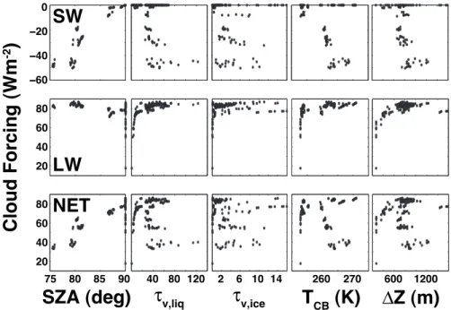
a function of solar zenith angle (SZA) as observed during M-PACE. As expected, short-wave cloud radiative forcing decreases with decreasing SZA (decreasing SZA means that the sun is higher in the sky). Cases for which the SZA was 90 are indicative of a sun that is at or below the horizon, and all calculated SZA values higher than 90 were set to 90 degrees. Longwave cloud radiative forcing is not shown to have the same 5

correlation. Perhaps there is some trend for higher SZA to result in lower longwave forcing, but this is likely due to decreases in temperature at later times of year. The second column from the left demonstrates the relationship between liquid optical depth and cloud radiative forcing. The most noticeable influence is on the longwave cloud forcing, with a sharp decrease in cloud forcing associated with very low optical depths. 10

This is due to contributions from the cold overlying atmosphere that are experienced at the surface when the cloud is not thick enough to mask those contributions. A similar effect can be seen with the ice water optical depth (center column), though it is not nearly as well-defined.

The effect of cloud base temperature is shown in the second column from the right. 15

As expected, lower cloud base temperatures result in decreased longwave cloud radia-tive forcing at the surface. In the cases presented, it appears as though clouds with the lowest liquid water optical depth also featured the lowest cloud base temperatures. For non-nighttime cases, shortwave cloud radiative forcing also demonstrates a decrease with increasing cloud base temperature. Analysis of the ratio of all-sky flux to clear sky 20

flux (not shown) demonstrates a similar increase with decreasing cloud base temper-ature. This implies that the relationship is due to a variety of factors, and that it is not due solely to colder clouds occurring later in the year. In support of this, thinner clouds were found to occur at colder temperatures. Longwave cloud radiative forcing demon-strates a relationship to cloud thickness similar to that of the liquid optical thickness. 25

(15)

ACPD

11, 12487–12518, 2011

forcing

G. de Boer et al.

Title Page

Tables Figures

◭ ◮

Back Close

Full Screen / Esc

Discussion

P

a

per

|

Dis

cussion

P

a

per

|

Discussion

P

a

per

|

Discussio

n

P

a

per

|

ratios than thicker ones. This implies that SZA differences between cases are masking the expected relationship between cloud thickness and cloud radiative forcing in Fig. 6. 3.3 Sensitivity tor_e

,liq, surface albedo andTsf c

Individual cases were analyzed in order to test the response of estimated surface fluxes to variables that are not able to be measured by the remote sensors themselves, such 5

asTsf c, surface albedo andre,liq. In the analysis performed above, estimates of surface

albedo and surface temperature were available from outside sources. In order to test the applicability of this technique in instances where similar measurements are not available, and to determine the sensitivity of the above estimates to the cloud base effective droplet size chosen, sensitivity tests were completed.

10

For the cloud base droplet effective radius, values between 3.5 µm and 10.5 µm were tested. The results of this comparison are demonstrated in Fig. 7. Due to the adia-batic assumption involved, the cloud-base droplet size will determine the droplet sizes throughout the rest of the cloud. This impacts mainly the shortwave radiation via a brightening of the cloud with smaller droplet sizes due to decreased absorption. This 15

effect is largest for case number one, where changing the cloud-basere,liqfrom 3.5 µm

to 10.5 µm results in an increase in downwelling shortwave flux of roughly 55 Wm−2. Cases 4, 6, 8, and 10 have similar sensitivity to this change, with surface downwelling fluxes increased by 25–35 Wm−2. Cases 11, 12, and 16 feature smaller sensitivities yet, with changes of 5–10 Wm−2. This decrease in sensitivity has less to do with cloud 20

properties than it does with larger and larger zenith angles occurring with the approach-ing Arctic night. As the pathlength through the atmosphere increases, and intensity of solar radiation reaching cloud top decreases, the brightening of clouds with smaller droplets has a smaller and smaller impact on the surface radiation. Similar patterns show up in the upwelling shortwave radiation, which is understandable due to its close 25

(16)

ACPD

11, 12487–12518, 2011

forcing

G. de Boer et al.

Title Page

Tables Figures

◭ ◮

Back Close

Full Screen / Esc

Discussion

P

a

per

|

Dis

cussion

P

a

per

|

Discussion

P

a

per

|

Discussio

n

P

a

per

|

In addition to changes in the shortwave radiation, there are also some impacts on longwave downwelling radiation. In general, these changes are minimal. The two ex-ceptions to this are cases 12 and 15, where there are reductions to the downwelling longwave radiation of 5 Wm−2 (2% of total) and 15 Wm−2 (7% of total) respectively. These are the thinnest cases sampled and the clouds impact on the downwelling long-5

wave radiation is not as dominant as for thicker clouds. In these instances, increasing there,liqdecreases the cloud optical depth, resulting in an increased contribution to the

downwelling surface longwave flux from the clear sky above cloud level, reducing the effective radiating temperature of the atmosphere. This results in decreased flux at the surface with increasingre,liq.

10

Surface shortwave fluxes also demonstrate significant sensitivity to the assumed surface albedo. Figure 8 demonstrates changes in downwelling shortwave flux of up to 80 Wm−2and up to 100 Wm−2in the upwelling surface shortwave radiative flux. These sensitivities came with changes in the surface albedo between 95% and 50%. The largest changes came at the upper end of this scale, with changes from 95% to 90%, 15

for example, resulting in larger decreases in surface shortwave flux than changes from 60% to 55%. Throughout the M-PACE experiment, as zolar zenith angle decreases, the sensitivity to surface albedo is reduced substantially. This is also evident when comparing the sensitivities from this study to those from Shupe and Intrieri (2004), who demonstrated a decreased surface flux of roughly 40 Wm−2for every 0.1 decrease in 20

surface albedo for conditions featuring a 60◦ SZA, 0.6 surface albedo and 50 gm−2 LWP. For case one conditions (SZA of 75◦, 0.6 surface albedo and 150 gm−2LWP) that sensitivity is closer to 5 Wm−2per 0.1 decrease in surface albedo due to the lower SZA and thicker cloud.

Sensitivity of results to surface temperature was also tested (not shown). Due to the 25

(17)

ACPD

11, 12487–12518, 2011

forcing

G. de Boer et al.

Title Page

Tables Figures

◭ ◮

Back Close

Full Screen / Esc

Discussion

P

a

per

|

Dis

cussion

P

a

per

|

Discussion

P

a

per

|

Discussio

n

P

a

per

|

surface flux of roughly 20 Wm−2. Integrated over a longer time period, this difference would eventually be detectable in the surface downwelling longwave flux due to a cooler atmosphere and cooler cloud temperature. The time frame required for a surface tem-perature change to significantly impact the downwelling longwave flux at the surface was not investigated in this study.

5

4 Summary

Cloud radiative forcing was estimated for mixed-phase clouds observed during M-PACE using a combination of modern cloud remote-sensors, current cloud measurements and retrievals and an advanced radiative transfer model. Using profiles of cloud prop-erties such as liquid and ice water paths, cloud heights, effective particle sizes and 10

temperature profiles to drive the radiative transfer model, a total of 16 mixed-phase cloud cases were evaluated. This technique was demonstrated to generally agree well with surface radiometric estimates, with the magnitude of most errors falling be-low 10 Wm−2. For shortwave radiation, errors were found to be largest for clouds with thicker liquid components, and were generally found to be negative, meaning the model 15

fluxes were too low when compared to the observations. Errors in downwelling long-wave radiation were largest for clouds with low liquid water paths, and generally posi-tive, meaning the model fluxes were too high compared to those observed.

The calculated fluxes were used to calculate cloud radiative forcing for these mixed-phase clouds. Shortwave forcing was generally small, due in part to the contribution 20

of nighttime cases, and in part to low sun-angles during this time of year. The largest shortwave forcing occurred early in the observation period and was roughly−50 Wm−2. Longwave cloud forcing was always positive, with most values falling between 70– 90 Wm−2. Combined with the shortwave forcing, this resulted in net cloud forcing rang-ing between 25–90 Wm−2. This demonstrates that these clouds act to warm the sur-25

(18)

ACPD

11, 12487–12518, 2011

forcing

G. de Boer et al.

Title Page

Tables Figures

◭ ◮

Back Close

Full Screen / Esc

Discussion

P

a

per

|

Dis

cussion

P

a

per

|

Discussion

P

a

per

|

Discussio

n

P

a

per

|

cloud forcing was demonstrated to correlate strongly with solar zenith angle, with an average change of 3 Wm−2 per degree. Shortwave cloud forcing also appears to be correlated with cloud-base temperature, although it is likely that this is a result of colder clouds occuring during times with lower solar zenith angles. Longwave cloud forcing was shown to be connected to both liquid optical depth and physical cloud thickness. 5

The relationship to liquid optical depth reaches an asymptote of roughly 85 Wm−2 for optical depths greater than 30 or so, while the relationship to cloud thickness reaches the same level for clouds thicker than 800 m.

The information presented here is relevant to understanding the impact of clouds on a changing surface state. The radiative impacts of specific cloud types on the freezing 10

and melting of sea ice, permafrost and glaciers, for example are just beginning to be explored. The results presented provide guidance on the use of this technique for expanding our knowledge of mixed-phase cloud forcing at observational sites that have cloud remote sensors but lack or have limited radiometric instrumentation. Future work will focus on application of this method to larger datasets, and exploration of the 15

radiative impact of mixed-phase stratiform clouds on surface ice melting rates. Doing so will provide information on the relevance of clouds and cloud-aerosol effects on the climate system, as well as help us to understand how simulated future changes in cloud types and cloud cover may impact the surface state.

Acknowledgements. The authors would like to thank Michael Iacono and the Atmospheric and

20

Environmental Research (AER) team for their help in getting RRTMG running propertly. In addition, we would like to thank the University of Wisconsin Lidar Group for making data from the M-PACE period available for evaluation via their website at http://lidar.ssec.wisc.edu, and the M-PACE crew for their hard work in compiling the datasets used. Funding for M-PACE was provided by the United States Department of Energy, and the current work is funded by the

25

(19)

ACPD

11, 12487–12518, 2011

forcing

G. de Boer et al.

Title Page

Tables Figures

◭ ◮

Back Close

Full Screen / Esc

Discussion

P

a

per

|

Dis

cussion

P

a

per

|

Discussion

P

a

per

|

Discussio

n

P

a

per

|

References

Barkstrom, B., Harrison, E., and Lee, R.: Earth Radiation Budget Experiment: Preliminary seasonal results, EOS, 71, 297, 1990. 12489

Clough, S., Shephard, M., Mlawer, E., Delamere, J., Iacono, M., Cady-Pereira, K., Boukabara, S., and Brown, P.: Atmospheric radiative transfer modeling: a summary of the AER codes, J.

5

Quant. Spectrosc. Radiat. Transfer, 91, 233–244, 2005. 12490

Curry, J. and Ebert, E.: Annual cycle of radiation fluxes over the Arctic Ocean: Sensitivity to cloud optical properties, J. Clim., 5, 1267–1280, 1992. 12489

Curry, J. and Herman, G.: Infrared radiative properties of summertime Arctic stratus clouds, J. Clim. Appl. Meteor., 24, 525–538, 1985. 12489

10

Curry, J., Rossow, W., Randall, D., and Schramm, J.: Overview of Arctic Cloud and Radiation Characteristics, J. Climate, 9, 1731–1764, 1996. 12489

de Boer, G., Tripoli, G. J., and Eloranta, E. W.: Preliminary comparison of CloudSAT-derived microphysical quantities with ground-based measurements for mixed-phase cloud research in the Arctic, J. Geophys. Res., 113, D00A06, doi:10.1029/2008JD010029, 2008. 12493

15

de Boer, G., Eloranta, E., and Shupe, M.: Arctic Mixed-Phase Stratiform Cloud Properties from Multiple Years of Surface-Based Measurements at Two High-Latitude Locations, J. Atmos. Sci., 66, 2874–2887, doi:10.1175/2009JAS3029.1, 2009. 12491

Dong, X. and Mace, G.: Arctic stratus cloud properties and radiative forcing derived from ground-based data collected at Barrow, Alaska, J. Clim., 16, 445–461, 2003. 12490, 12499

20

Dong, X., Xi, B., Crosby, K., Long, C., Stone, R., and Shupe, M.: A 10 year climatology of Arctic cloud fraction and radiative forcing at Barrow, Alaska, J. Geophys. Res., 115, D17212, doi:10.1029/2009JD013489, 2010. 12499

Donovan, D. and van Lammeren, A.: Cloud effective particle size and water content profile retrievals using combined lidar and radar observations I – Theory and examples, J. Geophys.

25

Res., 105, 27425–27488, 2001. 12493

Ebert, E. and Curry, J.: A parameterization of ice cloud optical properties for climate models, J. Geophys. Res., 97, 3831–3836, 1992. 12497

Eloranta, E.: High Spectral Resolution Lidar, in: Lidar: Range-Resolved Optical Remote Sens-ing of the Atmosphere, edited by: Weitkamp, K., 143–163, SprSens-inger-Verlag, 2005. 12491

30

(20)

ACPD

11, 12487–12518, 2011

forcing

G. de Boer et al.

Title Page

Tables Figures

◭ ◮

Back Close

Full Screen / Esc

Discussion

P

a

per

|

Dis

cussion

P

a

per

|

Discussion

P

a

per

|

Discussio

n

P

a

per

|

doi:10.1029/2000JC000439, 2002. 12503

IPCC: Climate Change 2007: The Physical Science Basis, Tech. rep., 2007. 12488

Kay, J. and Gettelman, A.: Cloud influence on and response to seasonal Arctic sea ice loss, J. Geophys. Res., 114, D18204, doi:10.1029/2009JD011773, 2009. 12488

Long, C. and Shi, Y.: An automated quality assessment and control algorithm for surface

radi-5

ation measurements, TOASJ, 2, 23–37, 2008. 12496

McFarquhar, G., Zhang, G., Poellot, M., Kok, G., McCoy, R., Tooman, T., Fridlind, A., and Heymsfield, A.: Ice Properties of Single-Layer Stratocumulus During the Mixed-Phase Arctic Cloud Experiment: 1. Observations, J. Geophys. Res., 112, D24201, doi:10.1029/2007JD008633, 2007. 12494

10

Moran, K., Martner, B., Post, M., Kropfli, R., Welsch, D., and Widener, K.: An unattended cloud-profiling radar for use in climate research, Bull. Am. Meteorol. Soc., 79, 443–455, 1998. 12491

Pinto, J.: Autumnal Mixed-Phase Cloudy Boundary Layers in the Arctic, J. Atmos. Sci., 55, 2016–2038, 1998. 12489

15

Prowse, T., Furgal, C., Wrona, F., and Reist, J.: Implications of climate change for northern Canada: freshwater, marine, and terrestrial ecosystems, Ambio, 38, 282–289, 2009. 12488 Ramanathan, V., Cess, R., Harrison, E., Minnis, P., Barkstrom, B., Ahmad, E., and Hartman,

D.: Cloud-radiative forcing and climate: Results for the Earth Radiation Budget Experiment, Science, 243, 57–63, 1989. 12498

20

Schweiger, A. and Key, J.: Arctic Ocean radiative fluxes and cloud forcing estimates from the ISCPP C2 cloud dataset, 1983–1990, J. Appl. Meteor., 33, 948–963, 1994. 12503

Shupe, M. and Intrieri, J.: Cloud radiative forcing of the Arctic surface: The influence of cloud properties, sufrace albedo, and solar zenith angle, J. Climate, 17, 616–628, 2004. 12490, 12495, 12499, 12502, 12503

25

Shupe, M., Matrosov, S., and Uttal, T.: Arctic Mixed-Phase Cloud Properties Derived from Surface-Based Sensors at SHEBA, J. Atmos. Sci., 63, 697–711, 2006. 12489, 12492 Shupe, M., Daniel, J., de Boer, G., Eloranta, E., Kollias, P., Long, C., Luke, E., Turner, D., and

Verlinde, J.: A Focus on Mixed-Phase Clouds: The Status of Ground-Based Observational Methods, Bull. Am. Meteorol. Soc., 87, 1549–1562, 2008. 12489, 12491

30

(21)

ACPD

11, 12487–12518, 2011

forcing

G. de Boer et al.

Title Page

Tables Figures

◭ ◮

Back Close

Full Screen / Esc

Discussion

P

a

per

|

Dis

cussion

P

a

per

|

Discussion

P

a

per

|

Discussio

n

P

a

per

|

Budget of the Arctic Ocean, Bull. Am. Meteorol. Soc., 83, 255–275, 2002. 12490

Verlinde, J., Harrington, J., McFarquhar, G., Yannuzzi, V., Avramov, A., Greenberg, S., Johnson, N., Zhang, G., Poellot, M., Mather, J., Turner, D., Eloranta, E., Zak, B., Prenni, A., Daniel, J., Kok, G., Tobin, D., Holz, R., Sassen, K., Spangenberg, D., Minnis, P., Tooman, T., Ivey, M., Richardson, S., Bahrmann, C., Shupe, M., De Mott, P., Heymsfield, A., and Schofield, R.:

5

The Mixed-Phase Arctic Cloud Experiment, Bull. Am. Meteorol. Soc., 88, 205–221, 2007. 12490

Zuidema, P., Baker, B., Han, Y., Intrieri, J., Key, J., Lawson, P., Matrosov, S., Shupe, M., Stone, R., and Uttal, T.: An Arctic Springtime Mixed-Phase Boundary Layer Observed During SHEBA, J. Atmos. Sci., 62, 160–176, 2005. 12492

(22)

ACPD

11, 12487–12518, 2011

forcing

G. de Boer et al.

Title Page

Tables Figures

◭ ◮

Back Close

Full Screen / Esc

Discussion

P

a

per

|

Dis

cussion

P

a

per

|

Discussion

P

a

per

|

Discussio

n

P

a

per

|

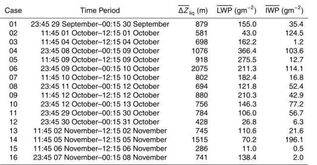
Table 1. Case overview providing case numbers, the time periods covered, and values for case mean liquid cloud depth, case mean liquid water path and case mean ice water path.

(23)

ACPD

11, 12487–12518, 2011

forcing

G. de Boer et al.

Title Page

Tables Figures

◭ ◮

Back Close

Full Screen / Esc

Discussion

P

a

per

|

Dis

cussion

P

a

per

|

Discussion

P

a

per

|

Discussio

n

P

a

per

|

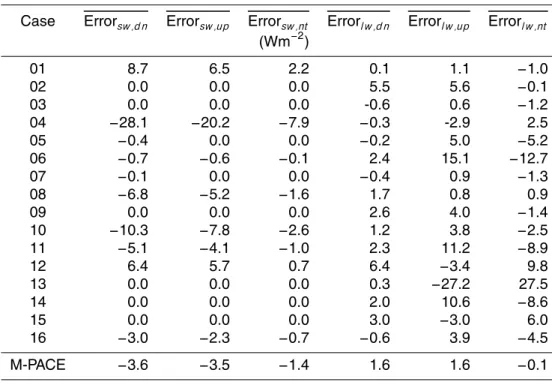
Table 2. Mean errors in modeled surface radiative fluxes (model-observation). Total shortwave error estimates do not include nighttime cases

Case Error_{sw,d n} Error_sw,up Error_sw,nt Error_{l w,d n} Error_{l w,up} Error_{l w,nt} (Wm−2)

01 8.7 6.5 2.2 0.1 1.1 −1.0 02 0.0 0.0 0.0 5.5 5.6 −0.1 03 0.0 0.0 0.0 -0.6 0.6 −1.2 04 −28.1 −20.2 −7.9 −0.3 -2.9 2.5 05 −0.4 0.0 0.0 −0.2 5.0 −5.2 06 −0.7 −0.6 −0.1 2.4 15.1 −12.7 07 −0.1 0.0 0.0 −0.4 0.9 −1.3 08 −6.8 −5.2 −1.6 1.7 0.8 0.9 09 0.0 0.0 0.0 2.6 4.0 −1.4

10 −10.3 −7.8 −2.6 1.2 3.8 −2.5

11 −5.1 −4.1 −1.0 2.3 11.2 −8.9

(24)

ACPD

11, 12487–12518, 2011

forcing

G. de Boer et al.

Title Page

Tables Figures

◭ ◮

Back Close

Full Screen / Esc

Discussion

P

a

per

|

Dis

cussion

P

a

per

|

Discussion

P

a

per

|

Discussio

n

P

a

per

|

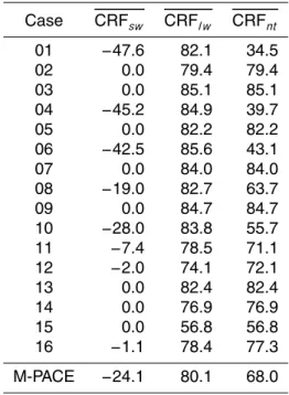
Table 3. Mean cloud radiative forcing for M-PACE mixed-phase clouds by case, and for the entire period. The M-PACE mean shortwave cloud radiative forcing does not include nighttime cases.

Case CRF_sw CRF_{l w} CRF_nt 01 −47.6 82.1 34.5

02 0.0 79.4 79.4 03 0.0 85.1 85.1 04 −45.2 84.9 39.7 05 0.0 82.2 82.2 06 −42.5 85.6 43.1 07 0.0 84.0 84.0 08 −19.0 82.7 63.7 09 0.0 84.7 84.7 10 −28.0 83.8 55.7 11 −7.4 78.5 71.1 12 −2.0 74.1 72.1 13 0.0 82.4 82.4 14 0.0 76.9 76.9 15 0.0 56.8 56.8 16 −1.1 78.4 77.3

(25)

ACPD

11, 12487–12518, 2011

forcing

G. de Boer et al.

Title Page

Tables Figures

◭ ◮

Back Close

Full Screen / Esc

Discussion

P

a

per

|

Dis

cussion

P

a

per

|

Discussion

P

a

per

|

Discussio

n

P

a

per

|

Time (UT)

Altitude (km)

11:50 11:55 12:00 12:05 12:10

0.4 0.8 1.2 1.6

(m str)1e−8-1

1e−7 1e−6 1e−5 1e−4 1e−3

% 1

5 10 50 100

0.4 0.8 1.2 1.6

dBZ

−30

−10 10

30

0.4 0.8 1.2 1.6

10 October 2004

0 0.1 0.2 0.3 0.4 0.5 0 0.01 0.02 0.03 0.04 0.05 0.06

0.4 0.8 1.2 1.6

Altitude (km)

LWC (gm-3₎ IWC (gm-3₎

AHSRL BSCS

AHSRL Depol

MMCR Reflectivity

0 20 40 60 80

Re,ice (µm) Re,liq (µm)

5

4 6

0.4 0.8 1.2 1.6

(26)

ACPD

11, 12487–12518, 2011

forcing

G. de Boer et al.

Title Page

Tables Figures

◭ ◮

Back Close

Full Screen / Esc

Discussion

P

a

per

|

Dis

cussion

P

a

per

|

Discussion

P

a

per

|

Discussio

n

P

a

per

|

0.4 0.8 1.2 1.6

∆

Zliquid฀

(k

m)

0 100 200

IWP

(gm

-2)

0 200 400

LWP

(gm

-2)

254 258 262 266 270

Tbase

(K)

20 40 60 80 4 5 6

2 4 6 8 10 12 14 16

Case Number re,liq

(

µ

m)

re,ice

(

µ

m)

(27)

ACPD

11, 12487–12518, 2011

forcing

G. de Boer et al.

Title Page

Tables Figures

◭ ◮

Back Close

Full Screen / Esc

Discussion

P

a

per

|

Dis

cussion

P

a

per

|

Discussion

P

a

per

|

Discussio

n

P

a

per

|

2 4 6 8 10 12 14 16

200 240 280

Case Number

Flux (Wm

-2 )

LWdown 30

60 90 230 260 290 20 40 60 −20 0 20 5 15 25

SW_down LWup

SW_up LWnet

SW_net

Modeled

Observed

−40

0

(28)

ACPD

11, 12487–12518, 2011

forcing

G. de Boer et al.

Title Page

Tables Figures

◭ ◮

Back Close

Full Screen / Esc

Discussion

P

a

per

|

Dis

cussion

P

a

per

|

Discussion

P

a

per

|

Discussio

n

P

a

per

|

LW Error (Model-Obs: Wm

-2)

SW Error (Model-Obs: Wm

-2)

−40 −20 0 20 40

−20 0 20

−10 0 10 20

DOWN

UP

NET

−30 −20 −10 0 10 20

0 4 8 12 τ_v,ice 0 40 80 120

−20 0 20

τ_v,liq

DOWN

UP

NET

−40 −20 0 20

16 160

(29)

ACPD

11, 12487–12518, 2011

forcing

G. de Boer et al.

Title Page

Tables Figures

◭ ◮

Back Close

Full Screen / Esc

Discussion

P

a

per

|

Dis

cussion

P

a

per

|

Discussion

P

a

per

|

Discussio

n

P

a

per

|

−100 −50 0 50 100

10 30 50 70 90

Cloud Radiative Forcing (Wm

-2

)

# of Profiles

Total Profiles: 151

LW

SW

NET

(30)

ACPD

11, 12487–12518, 2011

forcing

G. de Boer et al.

Title Page

Tables Figures

◭ ◮

Back Close

Full Screen / Esc

Discussion

P

a

per

|

Dis

cussion

P

a

per

|

Discussion

P

a

per

|

Discussio

n

P

a

per

|

75 80 85 90

SZA (deg)

40 80 120

τ

_v,liq 2 6 10 14

_T

260 270_CB

_(K)

_∆

600 1200

_{Z (m)}

Cloud Forcing (Wm

-2

)

−60 −40 −20 0

20 40 60 80

τ

_v,ice

SW

LW

NET

(31)

ACPD

11, 12487–12518, 2011

forcing

G. de Boer et al.

Title Page

Tables Figures

◭ ◮

Back Close

Full Screen / Esc

Discussion

P

a

per

|

Dis

cussion

P

a

per

|

Discussion

P

a

per

|

Discussio

n

P

a

per

|

2 6 10 14

0 40 80 120

Case Number

SW

200 240 280 320

2 6 10 14

3.5 µ

_m

4.5 µ

_m

5.5 µ

_m

6.5 µ

_m

7.5 µ

m

8.5 µ

_m

9.5 µ

_m

10.5 µ

_m

LW

Surface Flux (Wm

-2

)

DOWN

UP

(32)

ACPD

11, 12487–12518, 2011

forcing

G. de Boer et al.

Title Page

Tables Figures

◭ ◮

Back Close

Full Screen / Esc

Discussion

P

a

per

|

Dis

cussion

P

a

per

|

Discussion

P

a

per

|

Discussio

n

P

a

per

|

0.5

0.55

0.6

0.65

0.7

0.75

0.8

0.85

0.9

0.95

2 6 10 14

0 40 80 120

Case Number

SW

220 260 300

2 6 10 14

LW

Surface Flux (Wm

-2