www.biogeosciences.net/10/851/2013/ doi:10.5194/bg-10-851-2013
© Author(s) 2013. CC Attribution 3.0 License.
Biogeosciences
Geoscientific
Geoscientific
Geoscientific
Geoscientific
The Australian terrestrial carbon budget
V. Haverd1, M. R. Raupach1, P. R. Briggs1, J. G. Canadell.1, S. J. Davis2, R. M. Law3, C. P. Meyer3, G. P. Peters4, C. Pickett-Heaps1, and B. Sherman5
1CSIRO Marine and Atmospheric Research, P.O. Box 3023, Canberra ACT 2601, Australia 2University of California, Irvine, Dept. of Earth System Science, CA, USA
3CSIRO Marine and Atmospheric Research, PB1, Aspendale, Victoria 3195, Australia
4Center for International Climate and Environmental Research – Oslo (CICERO), P. B. 1129 Blindern, 0318 Oslo, Norway 5CSIRO Land and Water, P.O. Box 1666, Canberra ACT 2600, Australia
Correspondence to: V. Haverd ([email protected])
Received: 31 July 2012 – Published in Biogeosciences Discuss.: 12 September 2012 Revised: 14 December 2012 – Accepted: 26 December 2012 – Published: 7 February 2013
Abstract. This paper reports a study of the full carbon
(C-CO2)budget of the Australian continent, focussing on 1990– 2011 in the context of estimates over two centuries. The work is a contribution to the RECCAP (REgional Carbon Cycle Assessment and Processes) project, as one of numer-ous regional studies. In constructing the budget, we estimate the following component carbon fluxes: net primary produc-tion (NPP); net ecosystem producproduc-tion (NEP); fire; land use change (LUC); riverine export; dust export; harvest (wood, crop and livestock) and fossil fuel emissions (both territorial and non-territorial).
Major biospheric fluxes were derived using BIOS2 (Haverd et al., 2012), a fine-spatial-resolution (0.05◦) of-fline modelling environment in which predictions of CABLE (Wang et al., 2011), a sophisticated land surface model with carbon cycle, are constrained by multiple observation types.
The mean NEP reveals that climate variability and ris-ing CO2 contributed 12±24 (1σ error on mean) and 68±15 TgC yr−1, respectively. However these gains were partially offset by fire and LUC (along with other minor fluxes), which caused net losses of 26±4 TgC yr−1 and 18±7 TgC yr−1, respectively. The resultant net biome pro-duction (NBP) is 36±29 TgC yr−1, in which the largest con-tributions to uncertainty are NEP, fire and LUC. This NBP offset fossil fuel emissions (95±6 TgC yr−1)by 38±30 %. The interannual variability (IAV) in the Australian carbon budget exceeds Australia’s total carbon emissions by fossil fuel combustion and is dominated by IAV in NEP. Territo-rial fossil fuel emissions are significantly smaller than the rapidly growing fossil fuel exports: in 2009–2010, Australia
exported 2.5 times more carbon in fossil fuels than it emitted by burning fossil fuels.
1 Introduction
Full carbon budgets for land regions are significant for sev-eral reasons: they provide insights into terrestrial carbon cy-cle dynamics, including processes contributing to the net trend and variability in the terrestrial carbon sink; they place anthropogenic carbon and greenhouse gas inventories in a broader context; and they indicate how anthropogenic inven-tories change spatially across regions and temporally in re-sponse to climate variability and changes in land use and land management. This paper reports a study of the full carbon budget of the Australian continent, focussing on 1990–2011 in the context of estimates over two centuries. The work is a contribution to the RECCAP (REgional Carbon Cycle As-sessment and Processes) project (Canadell et al., 2011), as one of numerous regional studies being synthesised in REC-CAP.
A carbon budget for a land region can be expressed by equating the change in territorial storage of carbon CT per unit timetwith the net flux of carbon into the land surface: −dCT/dt= −dCB/dt−dCF F/dt−dCHWP/dt (1)
Changes in other C pools (e.g. biological products other than HWP) are considered negligible. The sign convention forF is that a positive flux is directed away from the land sur-face. (However note also the following hereafter: (i) positive “productivities” denoted e.g. NPP (net primary production), NEP (net ecosystem production), and NBP (net biome pro-duction); in the absence of the main symbolF are by defi-nition uptake by the land; (ii) positive “exports” and “emis-sions” are by definition fluxes away from the land surface.) Flux subscripts denote contributions to the net flux from NPP, heterotrophic respiration (RH), fire, land use change (LUC), transport by rivers and dust, harvest, fossil fuel emis-sions (FF), and FF export. It is assumed that, in all gaseous fluxes, C is present as C in CO2, and that the ultimate fate of C in the lateral fluxes (transport, harvest, exported FF) is C in CO2. (Hereafter C in CO2 will be abbreviated as C.) Terms in Eq. (1) can also be used to construct the net land-to-atmosphere C flux:
FLAE=FNPP+FRH+FFire+FLUC+FFF (2) +FHarvestConsump−dCHWP/dt,
where LAE denotes land–atmosphere exchange and FHarvestConsump is the component of the harvest flux that is consumed within the land region. The portion of the harvest that is consumed but does not decompose is accounted for by the change in stored HWP. The total change in atmospheric C storage attributable to loss of C from the land is given by−dCT/dt (Eq. 1), and is the sum ofFLAE and non-territorial (NT) emissions resulting from lateral fluxes (i.e. transport fluxes, and the export of harvest and FF). As such, a bottom-up estimate of dCT/dtformed by estimating the component fluxes provides an independent test of results from “top-down” atmospheric inversion approaches (Canadell et al., 2011).
The aim of this work is to construct a full carbon bud-get for the period 1990–2011 by combining estimates of the fluxes in Eq. (1). Methods for estimating the flux compo-nents are detailed in Sect. 2, and the budget is summarised in Sect. 3. Details of the component fluxes are presented in Sect. 4. In Sect. 5 atmospheric inversion results for Australia are discussed.
2 Methods and datasets
Net primary production and net ecosystem production were obtained using a regional biospheric modelling environment (BIOS2), subject to constraint by multiple observation sets (including eddy flux data and carbon pool data), as described in Sect. 2.1 below. We chose to use BIOS2 in preference to multiple estimates of NPP and NEP from global ecosystem models participating in the carbon cycle model intercom-parison project (TRENDY) (Sitch and Friedlingstein, 2011). The reason for this is that these global models exhibit vari-ability in Australian continental NPP estimates (2.2 PgCy−1
(range) and 0.8 PgCy−1(1σ )), which is much higher than the uncertainty (0.2 PgCy−1(1σ ))in the regionally constrained BIOS2 estimates (Haverd et al., 2012).
Most other components of the carbon budget were ob-tained independently as described in Sects. 2.2–2.6, with two exceptions. First, the heterotrophic respiration, which is de-rived primarily from BIOS2, is corrected for the influences of fire, transport (by river and dust) and harvest (Sect. 2.1). Second, the net fire emissions from non-clearing fires were estimated using a BIOS2 simulation with prescribed gross fire emissions (Sect. 2.2.2).
2.1 Net primary production, net ecosystem production and heterotophic respiration
NPP and NEP components were derived using BIOS2 (Haverd et al., 2012), constrained by multiple observation types, and forced using remotely sensed vegetation cover. BIOS2 is a fine-spatial-resolution (0.05◦) offline modelling environment built on capability developed for the Australian Water Availability Project (King et al., 2009; Raupach et al., 2009). It includes a modification of the CABLE land sur-face scheme (Wang et al., 2011) incorporating the SLI soil model (Haverd and Cuntz, 2010) and the CASA-CNP bio-geochemical model (Wang et al., 2010). BIOS2 parameters are constrained and predictions are evaluated using multiple observation sets from across the Australian continent, includ-ing streamflow from 416 gauged catchments, eddy flux data (CO2and H2O) from 12 OzFlux sites, litterfall data, and data on soil, litter and biomass carbon pools (Haverd et al., 2012). CABLE consists of five components (Wang et al., 2011): (1) the radiation module describes direct and diffuse radia-tion transfer and absorpradia-tion by sunlit and shaded leaves; (2) the canopy micrometeorology module describes the surface roughness length, zero-plane displacement height, and aero-dynamic conductance from the reference height to the air within canopy or to the soil surface; (3) the canopy module includes the coupled energy balance, transpiration, stomatal conductance and photosynthesis of sunlit and shaded leaves; (4) the soil module describes heat and water fluxes within soil and snow and at their respective surfaces; and (5) the ecosys-tem carbon module accounts for the respiration of secosys-tem, root and soil organic carbon decomposition. In BIOS2, the default CABLE v1.4 soil and carbon modules were replaced respec-tively by the SLI soil model (Haverd and Cuntz, 2010) and the CASA-CNP biogeochemical model (Wang et al., 2010). Modifications to CABLE, SLI and CASA-CNP for use in BIOS2 are detailed in Haverd et al. (2012).
Moreover, model structural errors incurred by process omis-sion are incorporated in the model-observation residuals, which are propagated through to uncertainties in model pre-dictions (Haverd et al., 2012).
In this work we extended BIOS2 simulations back in time to 1799, to assess the effects of changing climate and atmo-spheric CO2 on NPP and NEP. CASA-CNP carbon pools were initialised by spinning the model 200 times over a 39 yr period using NPP generated with atmospheric CO2 fixed at the pre-industrial value of 280 ppm, and 1911–1949 meteorology, corresponding to the earliest available rain-fall and temperature data from the Bureau of Meteorology’s Australian Water Availability Project dataset (BoM AWAP) (Grant et al., 2008; Jones et al., 2009). Following spin-up, the 1799–2011 simulation was performed using actual deseason-alised atmospheric CO2(from the Law Dome ice core prior to 1959 (MacFarling Meure et al., 2006), and from global in situ observations from 1959 onward (Keeling et al., 2001) with repeated 1911–1949 meteorology prior to 1911 and ac-tual meteorology thereafter.
Vegetation cover was prescribed using PAR (fraction pho-tosynthetic absorbed radiation) estimates obtained from the AVHRR record (1990–2006), with an annual climatology be-ing used outside of the period of data availability. Total fPAR was partitioned into persistent (mainly woody) and recur-rent (mainly grassy) vegetation components, following the methodology of Donohue et al. (2009) and Lu et al. (2003). Leaf area index (LAI) for woody and grassy components was estimated from the fPAR components by Beer’s law (e.g. Houldcroft et al., 2009). Grassy LAI was partitioned between C3 and C4 components according to the proportion of all grass species that are C4 species, as estimated by Hatters-ley (1983).
Uncertainties in BIOS2 predictions (all uncertainties here-after expressed as 1σ), due to parameter uncertainty and un-certainty in forcing data, were estimated separately and com-bined in quadrature to give total uncertainty, as described by Haverd et al. (2012). To obtain uncertainties in model predic-tions associated with parameter uncertainties in a parameter setp, the parameter covariance matrix C was projected onto the variance in the predictionZ:
σZ2=
∂Z ∂p
!T
C
∂Z
∂p (3)
where∂Z/∂p is the vector of sensitivities of a prediction
Z to the elements ofp. Uncertainties in model predictions associated with forcing uncertainties were estimated as the absolute change in prediction associated with perturbations to forcing inputs. NEP uncertainty estimates also include the uncertainty due to an assumed 20 % uncertainty in the partial derivative of NPP with respect to atmospheric CO2 concen-tration.
We define net ecosystem production as net primary pro-duction (NPP) minus the heterotrophic respiration flux that
would occur without the influences of fire, transport (by river and dust) and harvest,FRH,-F-T-H. (Here subscripts F, T, -H denote the absence of fire, harvest and transport.) Sec-tion 2.2 describes the estimaSec-tion ofFRH,-F-T-H, i.e.FRHunder a regime of fire. The effect of harvest and transport onFRHis treated more simply: we assumeFRHis discounted by 100 % of the exported flux, because the C in these fluxes is removed and cannot be respired.
2.2 Fire
2.2.1 Gross fire emissions
Gross monthly fire emissions were extracted from the GFED3 database (van der Werf et al., 2010) for the 1997– 2009 period. These emissions are determined using the al-gorithm of Sieler and Crutzen (1980), with burnt area deter-mined from the MODIS burned area product from 2002 to 2009 and from AVHRR for the period 1997–2002 (Giglio et al., 2010), fuel loads calculated using the CASA terrestrial biosphere model (Randerson et al., 1997) and combustion pa-rameters sourced from the global literature. These were com-pared with independent estimates derived using the 2004 Na-tional Greenhouse Gas Inventory Methodology (Australian Greenhouse Office, 2006; Meyer, 2004). This methodology also implements the algorithm of Sieler and Crutzen (1980). However the data are entirely independent of GFED. Burnt area in the tropical savanna and arid rangelands is estimated from AVHRR 1 km imagery (Craig et al., 2002) while, for the forests area, fire area estimates are sourced from fire agency statistics. In all regions fuel loads and combustion parameters are sourced from field measurements. The NGGI (National Greenhouse Gas Inventory) methodology is implemented re-gionally, by state (administrative unit), while GFED3 is spa-tially explicit at 0.5 deg resolution.
Uncertainty (1σ ) in continental gross fire emissions was estimated as the difference between the NGGI and GFED3, each averaged over the period (1997–2009) for which both products exist.
2.2.2 Net fire emissions
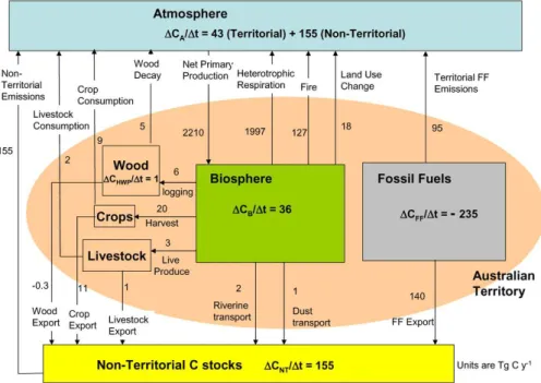
Fig. 1. Summary of the Australian territorial carbon budget, 1990–2011.
landscapes are resilient, with regrowth commencing after the first post-fire rainfall (Graetz, 2002).
For the purpose of estimating net fire emissions, clearing fire emissionsFfire, clearing were specified according to DC-CEE (2012) and subtracted from the gross fire emissions from GFED3 to give Ffire, non-clearing. The net export of C from the biosphere due to non-clearing fires was evaluated as
Ffirenet,non-clearing=Ffire,non-clearing−FRH,-F-T-H+FRH,-T-H (4)
=Ffire,non-clearing
1−FRH,-F-T-H−FRH,-T-H Ffire,non-clearing
.
Heterotrophic respiration under a recurring fire regime (but without account for transport by rivers and dust or harvest), FRH,-T-H, was estimated using a modification of the BIOS2 environment, in which (i) fire occurred at prescribed return intervals; (ii) at the time of fire, each aboveground carbon pool Cj was instantaneously depleted by fbβjCj with βj being a set of prescribed burning efficiencies for each above-ground pool andfbthe fraction of area burned. Burning ef-ficiencies were assigned according to values used by Bar-rett (2010). The fraction burned area was calculated as fb=
(rNPPt) P
j βjCj
(5)
withr a prescribed ratio of gross fire emissions to NPP (Ta-ble 2, Sect. 4.2.2 below) and NPPt the NPP accumulated since the last burn. Gross fire emissions in this simulation are thus equal torNPPt.
Relative uncertainty in the mean net fire emissions was assumed equal to that of the gross fire emissions.
2.3 Land use change and harvest
For land use change (LUC), flux estimates (FLUC)(1990– 2008) were extracted from the Australian National Green-house Gas Inventory (DCCEE, 2012), and associated data files (UNFCCC, 2011; v.1.4). The component extracted is the one consistent with the Kyoto Protocol article 3.3 which fo-cuses on emissions from deforestation and reforestation. Es-timates ofFLUCare calculated using the Australian National Carbon Accounting System (NCAS), a greenhouse account-ing framework for the land sector. It is based on spatially explicit ecosystem modelling that uses extensive ground-based datasets for parameterization and validation, and Land-sat data time series at 25-m resolution (Richards and Brack, 2004; Waterworth and Richards, 2008; Waterworth et al., 2007).
The LUC flux from NCAS includes emissions from con-verting forest to cropland and to grassland, and afforestation largely from the conversion of grasslands to forest land (i.e. plantations). The FullCAM model, used as part of NCAS, estimates emissions and removals from all pools including living biomass, dead organic matter, and soil (Richards and Evans, 2004).
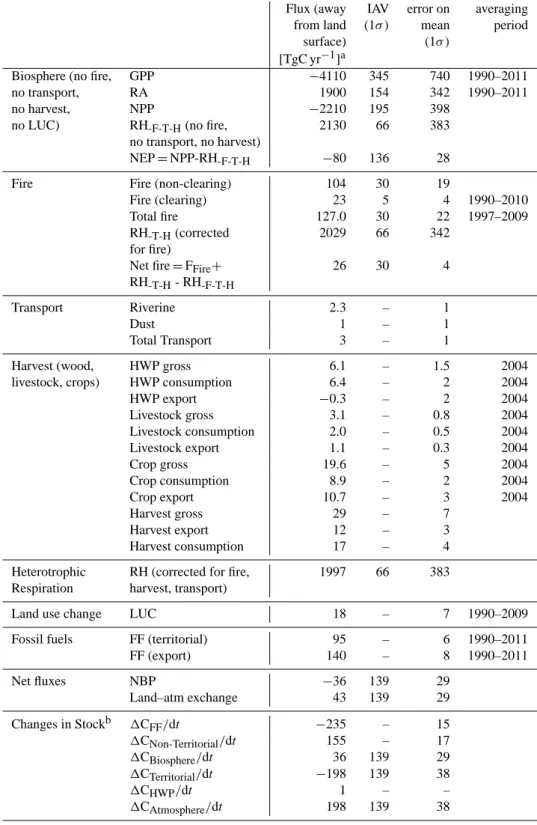
Table 1. Components of the Australian carbon budget.
Flux (away IAV error on averaging from land (1σ ) mean period
surface) (1σ ) [TgC yr−1]a
Biosphere (no fire, GPP −4110 345 740 1990–2011
no transport, RA 1900 154 342 1990–2011
no harvest, NPP −2210 195 398
no LUC) RH-F-T-H(no fire, 2130 66 383
no transport, no harvest)
NEP=NPP-RH-F-T-H −80 136 28
Fire Fire (non-clearing) 104 30 19
Fire (clearing) 23 5 4 1990–2010 Total fire 127.0 30 22 1997–2009 RH-T-H(corrected 2029 66 342
for fire)
Net fire=FFire+ 26 30 4
RH-T-H- RH-F-T-H
Transport Riverine 2.3 – 1
Dust 1 – 1
Total Transport 3 – 1
Harvest (wood, HWP gross 6.1 – 1.5 2004
livestock, crops) HWP consumption 6.4 – 2 2004
HWP export −0.3 – 2 2004
Livestock gross 3.1 – 0.8 2004
Livestock consumption 2.0 – 0.5 2004 Livestock export 1.1 – 0.3 2004
Crop gross 19.6 – 5 2004
Crop consumption 8.9 – 2 2004
Crop export 10.7 – 3 2004
Harvest gross 29 – 7
Harvest export 12 – 3
Harvest consumption 17 – 4
Heterotrophic RH (corrected for fire, 1997 66 383 Respiration harvest, transport)
Land use change LUC 18 – 7 1990–2009
Fossil fuels FF (territorial) 95 – 6 1990–2011
FF (export) 140 – 8 1990–2011
Net fluxes NBP −36 139 29
Land–atm exchange 43 139 29
Changes in Stockb 1CFF/dt −235 – 15
1CNon-Territorial/dt 155 – 17
1CBiosphere/dt 36 139 29
1CTerritorial/dt −198 139 38
1CHWP/dt 1 – –
1CAtmosphere/dt 198 139 38
aMultiply by 0.126 to convert to g m−2yr−1.
For harvested products, the Australian National Carbon Ac-counting System (NCAS) accounts for the change in stock of harvested wood products (HWP). This stock includes wood products from forest land within Australia plus imported ma-terial minus exported mama-terial. Descriptions of the methods and data sources are described in DCCEE (2012), and details of the wood products model and accounting framework are described in Richards et al. (2007).
Production, consumption and export of C in HWP, crops and livestock feed consumption were estimated using the methodology of Peters et al. (2012), applied to Australia for this work. The livestock feed consumption data were verted to carbon content of livestock using the livestock con-version efficiency factor (for Oceania) of 3.7 % from Krauss-mann et al. (2008) (Table 6).
For uncertainties of LUC emissions, we assumed the global value of 40 % (1σ ) (Le Quere et al., 2009), while for fluxes of harvested products, we assume uncertainties of 25 % (1σ).
2.4 Riverine transport
Freshwater fluxes of dissolved organic carbon (DOC), which we assume is of terrestrial origin, are computed as the prod-uct of a representative DOC concentration and the mean an-nual river flow.
River flow is taken to be either the modelled runoff from one of several significant recent studies of surface water re-sources in Australia (e.g. Raupach et al., 2009; CSIRO, 2008) or, for the catchments of the Great Barrier Reef lagoon, measured annual discharge from the Short Term Modelling Project (Cogle, Carroll, and Sherman, 2006) and from Fur-nas (2003).
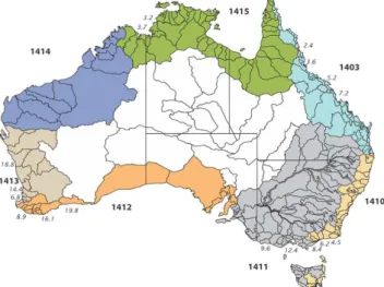
A database of DOC concentrations for Australian conti-nental rivers was assembled from the literature (e.g. Bass et al., 2011). These data were used to estimate mean DOC concentrations as follows: the Australian continent is broken up into 246 distinct hydrographic basins (a.k.a. surface wa-ter management areas) (ASWMA, 2004). Where data were available for more than one river within a basin, a flow-weighted mean concentration was computed from the ob-servations and assigned to the entire basin. This concen-tration was multiplied by the total basin runoff to give the DOC flux for the basin. For calculating fluxes to the ocean, the 246 basins were aggregated to areas contributing to 7 COSCAT zones (COastal Segmentation and related CATch-ments), based on a combination of coastal shelf morphology, coastal current patterns, and climate gradients (Meybeck et al., 2006), as shown in Fig. 13. Fluxes were calculated on a COSCAT zone basis as the product of the relevant annual runoff and a representative concentration. The representa-tive concentration was computed as a flow-weighted average from the constituent basins. In the absence of any measured DOC data, a value was assigned using judgement to
interpo-late between basins with observational data and considering the local landscape and hydrologic attributes.
In the absence of uncertainty estimates, we assign a rela-tive uncertainty of 50 % on this component of the C budget. This crude estimate has negligible impact on the uncertainty of NBP, because the C flux associated with riverine transport is very small (Sect. 4.4).
2.5 Dust export
Net dust export from Australia is equal to gross dust emis-sions minus wet and dry dust deposition terms. Estimates of these terms were obtained from a literature survey of stud-ies (Ginoux et al., 2004; Li et al., 2008; Luo et al., 2003; Miller et al., 2004; Tanaka and Chiba, 2006; Werner et al., 2002; Yue et al., 2009; Zender et al., 2003) that use global atmospheric/chemical transport models and/or climate mod-els, specifically enabled to simulate the uplift, transport and wet/dry deposition of dust. Li et al. (2008) specifically tar-get regions in the Southern Hemisphere. Of the eight stud-ies, only four provided full dust budgets. The mean ratio of net dust export to gross dust emissions for Australia obtained from these four studies was applied to the gross emissions of the remaining four studies.
Export of carbon by dust is estimated by multiplying net dust export by a fixed soil organic content (SOC) of dust, taken as 4±3 %. This value is based on a range of 1–7 % SOC observed in wind-blown sediment samples in a recent study indicating significant enrichment of carbon in Aus-tralian dusts relative to parent soils (Webb et al., 2012).
Uncertainty in this flux component of the C budget is as-sumed as 100 % of the flux, based on the large uncertainty in the soil organic carbon content of dust and the large range of net dust export estimates (Sect. 4.5). This crude estimate has negligible impact on the uncertainty of NBP, because the C flux associated with dust transport is very small (Sect. 4.5).
2.6 Fossil fuel
Table 2. Ratio of annual gross fire emissions and annual net fire
emissions to mean NPP (1990–2011): mean ratio; IAV of ratio and maximum ratio for the 1997–2009 period.
Gross fire emissions/ Net fire emissions/
mean NPP mean NPP
mean IAV (1σ ) max mean IAV (1σ ) max
Tropics 0.18 0.04 0.24 −0.015 0.003 0.001
Savanna 0.09 0.03 0.15 −0.002 0.0006 0.000
Warm Temp 0.01 0.01 0.05 0.008 0.008 0.030
Cool Temp 0.03 0.04 0.14 0.016 0.022 0.075
Mediterranean 0.006 0.003 0.01 1.8×10⁻⁵ 8×10⁻⁶ 3×10⁻⁵
Desert 0.03 0.02 0.07 0.004 0.002 0.0089
Australia 0.06 0.02 0.08 0.0014 0.003 0.0074
consumption is known relatively accurately, the uncertainty of carbon content of coal is∼6 %.
3 The net carbon budget, 1990–2011
Table 1 summarises the net territorial Australian carbon bud-get, and it is further distilled in Figs. 1 and 2. Each compo-nent is discussed in detail in Sect. 4.
The budget period for each flux component is specified as 1990–2011, and is defined as starting at the beginning of 1990 or whenever data become available thereafter, and end-ing at the end of 2011, or whenever data cease beend-ing avail-able before then. Estimates of NPP and NEP span the entire budget period. Of the remaining fluxes, it is mostly assumed that the average flux over the available years applies to the entire budget period. The exception is fossil fuel emission and export, for which the 1990–2011 values were derived by extrapolation (Sect. 2.6).
For the 1990–2011 period, the biosphere gained carbon at an average rate of 36±29 TgC yr−1 (1σ error on mean). As indicated in Figs. 1 and 2i, the gross loss of carbon from the biosphere is dominated by heterotrophic respira-tion (1997±383 TgC yr−1), with smaller losses due to fire (127±22 TgC yr−1), harvest (29±7 TgC yr−1), land use change (18±7 TgC yr−1) and transport by rivers and dust (3±1 TgC yr−1). However the process contributions to bio-spheric carbon accumulation are quite different. As shown in Fig. 2ii, the net effects of changing climate and ris-ing CO2 are to increase biospheric carbon by 12±24 and 68±7 TgC yr−1respectively, while fire and LUC cause net respective losses of 26±4 TgC yr−1 and 18±7 TgC yr−1. (Harvest and transport are assumed to have no net effect on biospheric carbon accumulation.)
Of the total harvest, 60 % is consumed in Australia and mostly contributes directly to the flux from the Australian territory to the atmosphere. A small part of the wood har-vest flux contributes to the accumulation of the HWP stock at a rate of 1 TgC yr−1. The exported harvest is returned to the atmosphere as non-territorial emissions. Small exports of carbon by river (2±1 TgC yr−1)and dust (1±1 TgC yr−1) transport also contribute to non-territorial emissions.
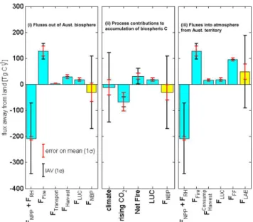
Fig. 2. (i) Net flux of carbon out of the Australian biosphere (FNBP,
yellow) as the sum of components (blue); (ii) net flux of carbon out of the Australian biosphere (FNBP, yellow) as the sum of process
contributions (blue) due to variable climate, rising CO2, net effect
of fire (mainly clearing fires) and LUC; (iii) net flux of carbon from the Australian territory to the atmosphere (FLAE, yellow), as the
sum of components (blue). Error bars represent errors on the mean (1σ, red) and interannual variability (1σ, black).
During the same period, the stock of carbon in fos-sil fuels was depleted by 235±15 TgC yr−1, of which 95±6 TgC yr−1 were attributable to burning of fossil fu-els within the Australian territory, and the remainder to ex-port. Combining territorial fossil fuel emissions with harvest consumption and biospheric land-to-atmosphere fluxes re-sults in a total land-to-atmosphere flux of 43±29 TgC yr−1, with an additional 155±17 TgC yr−1contribution from non-territorial emissions resulting from consumption of Aus-tralian harvest and fossil fuels outside of Australia.
Components of the net flux out of the Australian biosphere and the net land-to-atmosphere flux are shown in bar-chart form in Fig. 2i and iii, along with their 1σ uncertainties and interannual variabilities (IAV). The IAV of both net fluxes is dominated by IAV in FNPP+FRH(136 TgC yr−1), which in turn is largely attributable to IAV in NPP (Table 1).
4 Components of the net carbon budget
4.1 NPP and NEP
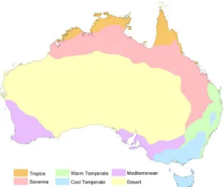
Fig. 3. Bioclimatic classification for use in regionalisation of
re-sults.
annual temperature and precipitation (1975–2011) for each bioclimatic region.
4.1.1 Spatial distribution of mean NPP
Figure 4 shows the spatial distribution of mean NPP (1990– 2011) at 0.05◦spatial resolution across the Australian
con-tinent, as simulated using BIOS2. Spatially and temporally variable drivers are meteorological inputs (air temperature, incoming solar radiation, precipitation), vegetation cover (to-tal leaf area index and its partition into woody and grassy components) and soil properties (temporally invariant). Solid lines in Fig. 4 indicate the boundaries of the bioclimatic re-gions (Fig. 3) and emphasise the strong climate dependence of NPP. The NPP is strongly weighted to the eastern, northern and south-western margins of the continent, with the remain-der of the continent having very low mean NPP.
4.1.2 Ranking the 1990–2011 period
It is important to assess the 1990–2011 period in the context of longer-term variability. Figure 5 shows the annual tem-poral variations of continental mean precipitation, NPP, and NEP, for 1911–2011. Precipitation is included because it is the single largest driver of variability in the Australian car-bon cycle. We assessed the representativeness of precipita-tion, NPP and NEP during 1990–2011 compared with other 22-yr periods in Fig. 5. The assessment was done by (i) con-structing moving average and standard deviation time series of each quantity using a 22-yr window period; and (ii) con-verting each point in the time series to a percentile rank (i.e. the percentage of points in the time series that have lower values than the point in question).
Results are shown in Fig. 6, for each bioclimatic region of Fig. 3 and for the whole continent. The final point in each time series is the percentile rank for the 1990–2011 period.
Fig. 4. Mean NPP (1990–2011), with boundaries of bioclimatic
re-gions (Fig. 3, Table 5) indicated as solid lines.
Table 3. Spatial extent, mean annual temperature and precipitation
of the bioclimatic regions shown in Fig. 3.
Area Fractional Mean annual Mean annual [106km2] area T (1975–2011) precip.
[%] [◦C] (1975–2011) [mm yr−1]
Tropics 0.39 5.07 26.4 1345
Savanna 1.62 21.31 24.2 704
Warm Temperate 0.32 4.27 17.2 808
Cool Temperate 0.34 4.47 12.4 881
Mediterranean 0.55 7.22 16.8 420
Desert 4.39 57.66 21.8 296
The x-axis represents the centre year of each 22-yr period. Several features emerge from Fig. 6: (i) at the decadal time scale, NPP is strongly correlated with precipitation; (ii) vari-ability in NEP is more noisy (occurs at shorter time scales) than variability in NPP; (iii) Mediterranean, cool temperate and warm temperate regions have experienced below-median rainfall in each 22-yr period from 1986 onwards (includ-ing 2010–2011, widely perceived as the break of a major drought from 2000–2009); (iv) in contrast, the tropics, sa-vanna, desert and the continent as a whole have experienced above-median rainfall during the same period; (v) the rank-ings of precipitation and NPP for the whole of Australia are very similar to those for the desert region; (vi) continental NEP reveals additional structure not seen in the desert, par-ticularly a decline in the periods from 1986–1997, associated with the tropics and savanna regions.
Fig. 5. Annual time series of Australian continental (i)
precipita-tion; (ii) NPP; and (iii) NEP (NPP – RH in the absence of fire and harvest). Shading represents 1σ uncertainties on the mean, and in-cludes contributions from parameter uncertainties and forcing un-certainties, as evaluated in Haverd et al. (2012).
and the whole of Australia (CP>85 %), but less so in the tropics, where variability in temperature (particularly its in-fluence on vapour pressure deficit) strongly inin-fluences vari-ability in NPP and NEP; (iii) the cool temperate region suf-fered from exceptionally low precipitation (CP<10 %) and NEP (CP<3 %), as a consequence of preceding decades of below-median NPP (Fig. 6).
4.1.3 Mean NPP 1990–2011
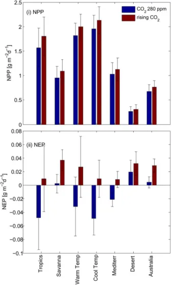
Mean NPP for each bioclimatic region and for the whole of Australia is shown in Fig. 8i, simulated at constant CO2 (280 ppm, a pre-industrial concentration), and with actual (rising) CO2. Error bars represent 1σ uncertainties due to uncertainties in model parameters and forcing. The param-eter uncertainty component represents the constraint on NPP predictions provided by multiple observation sets in the pa-rameter estimation process (Haverd et al., 2012). The Aus-tralian continental mean value (with rising CO2forcing) on a per unit area basis is 0.76 g m−2d−1, equivalent to 73 % of the global mean of 1.04 g m−2d−1for a global land NPP of 55 PgC yr−1(Cramer et al., 2001) and 56±14 PgC yr−1(Ito, 2011). This is taking Australia as 5.5 % of the global land area, and excluding Greenland and Antarctica. Rising CO2 increases continental NPP by 13 % compared with steady preindustrial forcing. Higher increases of 15–16 % occur in the tropics, savanna and desert (which are subject to very high temperatures and humidity deficits) and lower values of 9–10 % in the temperate and Mediterranean regions. The response of NPP to rising CO2is also shown in time series
Fig. 6. Percentile rank time series of 22-yr averaged precipitation,
NPP and NEP. Each point is the percentile rank of the variable (pre-cipitation, NPP or NEP), averaged over a 22-yr window, centered at the time on the x-axis. A point having a percentile rank of 100 % means that all other points in the time series have lower values.
form in Fig. 8i. Each time series is the difference between NPP simulated at “rising CO2” and “constant CO2”, relative to the “constant CO2” NPP.
4.1.4 Mean NEP 1990–2011
Fig. 7. Percentile ranks of the 1990–2011 (i) mean and (ii) standard deviation of precipitation, NPP and NEP, relative to all other 22-yr
periods starting in successive years from 1911.
Responses of NEP to CO2are plotted in Fig. 9ii. Interan-nual variations in the NPP responses (Fig. 9i) are amplified in the NEP responses because of the time delay between a change in NPP and the consequent change in RH. For clarity, the responses are replotted in Fig. 9ii (inset) as 22-yr running means, revealing distinct responses for the different regions. The largest response is in the desert region (4.5 % of NPP in 2011), and the response for Australia is 3.5 % of NPP in 2011.
Fig. 8ii shows that, with constant CO2 forcing, the trop-ics, warm temperate and cool temperate regions would be significant sources of CO2 to the atmosphere, because the averaging period (1990–2011) is preceded by a long pe-riod of declining NPP (Fig. 6). However, the CO2 re-sponse is sufficiently strong that each bioclimatic region, and the whole of Australia, is a net sink under a regime of no disturbance. Error bars represent the 1σ uncertain-ties in NEP resulting from 20 % uncertainty in the partial derivative of NPP with respect to atmospheric CO2 concen-tration, combined in quadrature with uncertainties due to uncertainties in model parameters and forcing. The conti-nental NEP values of 0.004 g m−2d−1 (constant CO2) and 0.029 g m−2d−1(rising CO2) are equivalent to respective continental sinks 12 TgC yr−1and 80 TgC yr−1. The sink un-der rising CO2 is 59 % of the mean terrestrial global sink (assuming a 1990–2011 average global sink of 2.6 PgC yr−1 (Canadell et al., 2007; Pan et al., 2011), and taking the Aus-tralian land surface are as 5.5 % of the global land surface, excluding Greenland and Antarctica). However the com-bined effects of fire and LUC (Fig. 2ii) reduce the continental biospheric sink to 36 TgC yr−1or 27 % of the global mean sink per unit area.
4.1.5 Interannual variability
As seen in the time series of Fig. 5, interannual variability (IAV) of continental NPP and NEP is strongly associated
with IAV in rainfall. For the 1990–2011 period, IAV (1σ )of NPP, relative to mean NPP, is 9 % for the continent, with high values of 14–15 % in the savanna, warm temperate, Mediter-ranean and desert regions, and lower values of 8 % in the tropics and cool temperate regions. The IAV of NEP is sim-ilar in absolute magnitude to that of NPP, with a continental value of 8 %, relative to mean NPP.
4.2 Fire
4.2.1 Gross fire emissions
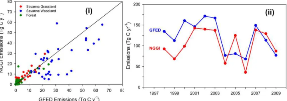
Figure 10i compares gross annual fire emissions derived us-ing the GFED and NGGI methodologies. Each point repre-sents an annual state (administrative unit) flux from one of three vegetation classes. The two estimates generally agree well, particularly for the forest and arid rangelands where the NGGI estimates are 20 % lower and 9 % higher respectively than the GFED estimates. The comparison of the savanna woodland estimates is slightly more complex. In this region, the Queensland fuel loads were prescribed by state experts while, for Northern Territory and Western Australia, they were based on field measurements. It is now clear that the Queensland estimates were biased towards heavily grazed re-gions of Western Queensland where the fuel loads are low in comparison to Cape York Peninsula where most fires occur. Excluding the Queensland data, NGGI estimates for tropi-cal savanna woodland are on average 13 % lower than GFED estimates. Annual continental fire emissions (Fig. 10ii) also agree very well, with a mean bias of 17 % of GFED with respect to NGGI.
Fig. 8. (i) BIOS2 estimates of 1990–2011 mean NPP under
pre-industrial CO2 and increasing CO2forcing. (ii) BIOS2 estimates
of 1990–2011 mean NEP under pre-industrial CO2and rising CO2.
Error bars represent 1σuncertainties on the mean, and include con-tributions from parameter uncertainties and forcing uncertainties, as evaluated in Haverd et al. (2012).
from west to east across the top end, corresponding to a time lag in the onset of the dry season. During the dry season, the air flows to the north-west from the arid rangelands in central Australia to the Timor Sea and the fetch across the arid interior to north-west Western Australia is particularly long. Hence this region becomes fire prone very early in the season, in contrast to the north east (Cape York, Queens-land) where winds are east to south-east, sometimes off the ocean and therefore more humid. The seasonality of fire in the rangelands is more variable than in the tropics; in the south fires occur more frequently in the summer. In the north, the seasonality of monsoons is the main driver.
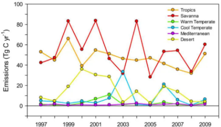
Figure 12 shows time series of the GFED3 annual gross fire emissions by region. The tropics are a persistently high source of gross fire emissions, while the savanna fire
emis-Fig. 9. (i) Response of NPP to increasing CO2, calculated as the
dif-ference between NPP simulated with rising CO2and pre-industrial
CO2(280 ppm), relative to NPP simulated with pre-industrial CO2;
(ii) response of NEP to increasing CO2, calculated as the difference
between NEP simulated with rising CO2and pre-industrial CO2, relative to NPP simulated with pre-industrial CO2.
sions are similarly high but show higher IAV, because fuel loads are more variable. The fire events in the desert coin-cide with years of high NPP associated with large rainfall events; the extreme fire years of 2000 and 2001 followed sev-eral extremely wet years in central Australia between 1997 and 1999.
The cool temperate region, usually a small source of fire emissions, produced large emissions in the severe bush-fire seasons of 2003 and 2006 during a period of extended drought (seen above in Fig. 6).
In Table 2, we list the mean fraction of NPP burned by region, its variability (1σ ), and maximum value. On average, biomass burning represents 6 % of continental NPP, slightly less than the IAV (1σ )of continental NPP (9 %, Sect. 3.1.4) or continental NEP (8 %, Sect. 3.1.4). At 2 % of NPP, the IAV (1σ )of gross fire emissions is small compared to that of NPP or NEP.
4.2.2 Net fire emissions
Annual gross fire emissions from non-clearing fires were ad-justed using Eq. (4) to obtain net annual emissions from these fires. The correction factor in Eq. (4) was approxi-mated as1−FRH,-F-T-H−FRH,-T-H
rNPPt
Fig. 10. Comparison of GFED3 and NGGI CO2-C gross fire emission estimates. (i) Annual fluxes per state per vegetation class; (ii) total
annual Australian continental fire emissions 1997–2009.
temperate and cool temperate) and 20 yr (Mediterranean and desert).
Results for each region and for the Australian continent are listed in Table 2. Net emissions are typically less than 5 % of gross emissions, indicating that, over the averaging period of interest (1990–2011), the C lost due to burning fuel is ap-proximately matched by the additional heterotrophic respira-tion that occurs in the absence of fire. Significant exceprespira-tions are the warm and cool temperate regions, where net fire emis-sions account for about 60 % of gross fire emisemis-sions. The rea-son for this large fraction is that, owing to the long fire return interval (50 yr), the biosphere does not recover to its pre-fire state within the averaging period (22 yr). Net fire emissions in the tropics and savanna are slightly negative. This does not mean that fire is increasing the uptake of biospheric carbon in the long term. On the contrary, in the absence of fire more carbon is sequestered in the soil over hundreds of years pre-ceding the 1990–2011 period. Because of this and because the period 1990–2011 occurs after an extended decline in NPP (Fig. 7), more C is temporarily being released as RH during 1990–2011 in the simulations with no fire than in the simulations with fire.
The net fire emissions in Table 2 need to be augmented by emissions from clearing fires. Graetz (2002) estimated these to be 18±10 PgC yr−1(IAV, 1σ ) which is close to the cur-rent estimate of 23±5 PgC yr−1 for 1990–2010 (DCCEE, 2012). Gross emissions from these fires are converted en-tirely to net emissions (Graetz, 2002).
4.3 Land use change and harvest
Net cumulative emissions from land use change were 359 TgC during the 1990–2009 period with mean annual emissions of 21.4 TgC for the 1990s and 14.4 TgC for the 2000s.
This cumulative net flux over 20 yr was the result of two major land use changes, the first being the conversion of for-est to grassland (12.9 Mha; 359 TgC) and forfor-est to cropland (4.4 Mha; 47 TgC) (Fig. 11). This dominant flux remained quite stable on average throughout the period after an initial
decline of 51 % during the period 1990–1995. The flux also takes into account the dynamics of regrowth and re-clearing of forest land, which takes place particularly in the northeast of Australia.
Second, the expansion of new forest largely results from the conversion of grasslands to forest, which creates a CO2 sink (1.1 Mha;−47.9 TgC) (Fig. 11). This flux was largely driven by the increase of plantations, which grew from about 1 Mha in 2003 to 1.8 Mha in 2006, largely attributable to the expansion of hardwood plantations, mainly Eucalyp-tus (Montreal Process Implementation Group for Australia, 2008).
Carbon fluxes for non-CO2greenhouse gases are negligi-ble for this type of land conversions and not part of the ac-counting of this paper.
The change in stock of harvested wood products1CHWP accounts for a small carbon sink in the context of other ma-jor fluxes reported for the Australian terrestrial carbon bud-get.1CHWP was estimated at 1.4 TgC in 1990, declining to 1.2 TgC in 2009 (DCCEE, 2012). We use an annual average across the period 1990–2009 of 1.3 TgC yr−1.
Production, consumption and export of in HWP, crops and livestock are given in Table 1 for the year 2004, as esti-mated by Peters et al. (2012), and extracted for Australia for this work. Of these harvest types, crops dominate pro-duction (19 TgC yr−1), with smaller productions of HWP (6.4 TgC yr−1)and livestock (3.1 TgC yr−1). In 2004 there was a net import of HWP (6 % of production), while 45 % of crop production and 63 % of livestock production were ex-ported.
4.4 Riverine transport
Fig. 11. Ensemble average GFED CO2-C gross fire emissions 0.5◦×0.5◦grid cell (1997–2009) by month.
the Australian coastline is estimated to be 2.3±1 TgC yr−1. This number is a preliminary estimate and could be refined as more DOC concentration data become available (presently available for only 33 of the total 246 basins).
Runoff estimates for Australia differ by roughly±5 % (not shown) suggesting a relatively small error in flux esti-mates is attributable to uncertainty in runoff. Far greater un-certainty can be attributed by the relatively large range of measured values for any given river. This variability must stem in part from the timing of flow events relative to field sampling. Field sampling on a weekly or less frequent basis may miss a significant proportion of the total DOC flux. Bass et al. (2011) suggest that insufficient temporal resolution of DOC measurements can lead to underestimating the flux by a factor of two or more.
There are several significant complications which are not accounted for in the above approach. First, there is no dis-tinction between the DOC flux in the significant portion of runoff that does not reach the sea and that which does. This is probably important: for example, of an estimated 27 041 GL yr−1of gauged runoff within the Murray–Darling Basin, just 4733 GL reach the ocean (CSIRO, 2008). Sec-ond, there is a chance that the typical DOC concentrations re-ported (and used here) have missed the initial surge of leach-ing and remineralisation which is likely to occur within the first few days of rainfall or flooding after an extended dry pe-riod (Glazebrook and Robertson, 1999; Hladyz et al., 2011). Third, remineralisation of DOC as water moves downstream along a river is not accounted for, and is probably important because the fraction of total organic carbon present as DOC can be highly variable (e.g. Vink et al., 2005).
Fig. 12. Annual time series of GFED CO2-C gross fire emissions by bioclimatic region.
Table 4. Mean annual runoff (Raupach et al., 2009) draining into
Australian COSCAT regions (Fig. 13), mean DOC concentrations computed from observed concentration data (italics denote assumed DOC concentration used to compute DOC fluxes), and DOC fluxes computed using each of the three runoff estimates. Fluxes were cal-culated using the maximum concentration observed in region 1411.
COSCAT Number Runoff Mean DOC DOC flux region of basins [GL yr−1] [mg/L] [GgC yr−1]
n/ainterior 31 4830 12 58
1403 62 76 273 6.3 481
1410 37 40 157 5 201
1411 95 79 600 3–13.4 1067
1412 18 3869 12.8 50
1413 13 2077 13.0 27
1414 14 18 284 5 91
1415 55 128 840 2.6 335
Total 325 353 931 2309
4.5 Dust transport
Table 5. Australian continental dust: annual emission, deposition, export and emission as % global emission.
Reference Emission Total Export % Dry Wet % global [Tg yr−1] Depos. [Tg yr−1] exported depos. depos. emission
[Tg yr−1] [Tg yr−1] [Tg yr−1]
Tanaka and Chiba (2006) 106 106 0 0.0 65 41 5.7
Luo et al. (2003) 132 129 3 2.3 70 59 8.0
Miller et al. (2004) 148 46 102 68.9 44 2 15.0
Yue et al. (2009) 73 46 27 37.0 38 8
Zender et al. (2003)∗ 37 27 10 27.0 2.5
Ginoux et al. (2004∗ 61 45 16 27.0 2.9
Li et al. (2008)∗ 120 88 32 27.0 5.2
Werner et al. (2002)∗ 52 38 14 27.0 4.9
Mean 91 65 26 27.0 6.3
SD 41 37 33 30 4.2
∗Full dust budget not published. Export and total deposition calculated assuming Export accounts for 27 % of Emission.
Fig. 13. Australian water catchments grouped by COSCAT zones
(filled colours). Bold numbers denote COSCAT zones. Italicised numbers denote representative DOC concentrations [mg L−1] from measurements taken in adjacent catchment rivers. COSCAT zones are based on a combination of coastal shelf morphology, coastal current patterns, and climate gradients (Meybeck, Durr, and Voros-marty, 2006).
within the Southern Hemisphere is due to the short atmo-spheric lifetime of dust.
Dust emissions peak from October–February and the ma-jor source regions within Australia are the Great Artesian Basin in Central Australia and the Murray–Darling Basin (Li et al., 2008; Maher et al., 2010). Dust emission and export are also characterized by short-lived, sporadic, intense events, sometimes resulting in short-lived, offshore ocean fertiliza-tion due to high iron content (Luo et al., 2008). The major pathways of dust export are to the south-east of the continent and, to a lesser extent, the north-west (Maher et al., 2010).
Fig. 14. Annual CO2-C fluxes from land use change (TgC).
Both total emission estimates and the fraction of dust ex-ported from Australia vary considerably (Table 5). Of the 8 emission estimates provided in Table 5, only four are accom-panied by a full budget, leading to a mean estimate of 27 % of dust emissions being exported out of Australia. Applying this estimate of 27 % to the remaining 4 emission estimates pro-vides a set of 8 estimates of the total mass of dust exported from Australia annually. The mean annual estimate of dust export from Australia is 26±33(1σ) Tg yr−1. The remain-ing dust is deposited elsewhere on the Australian continent, primarily through dry deposition (Yue et al., 2009; Tanaka and Chiba, 2006; Luo et al., 2003), although the proportion of dry vs. wet deposition varies significantly.
Assuming a dust carbon content of 4±3 % (Sect. 2.5 above) and a 100 % uncertainty estimate on net dust export leads to an estimate of 1±1 TgC yr−1.
4.6 Fossil fuel emissions
Fig. 15. Millions of tons (Mt) of CO2embodied in trade in 2004.
The upper panel shows regional differences between extraction and production emissions (i.e. the net effect of emissions from traded fossil fuels), and the lower panel shows regional differences be-tween production and consumption emissions (i.e. the net effect of emissions embodied in goods and services). Net exporting coun-tries are shown in blue and net importing councoun-tries in red. Arrows in each panel depict the fluxes of emissions (Mt CO2yr−1)to and
from Australia greater than 9 Mt CO2yr−1. Fluxes to and from
Eu-rope are aggregated to include all 27 member states of the EuEu-ropean Union.
basis, Australia’s total GHG emissions in 2009–2010, ex-cluding net CO2emissions from land use, land use change and forestry (LULUCF), were 148 TgC-equivalent yr−1, or 543 TgCO2-equivalent yr−1in the units conventionally used in greenhouse accounting (DCCEE, 2012). These CO2 -equivalent emissions include all Kyoto GHGs (CO2, CH4, N2O, HFCs, PFCs, SF6). Of these emissions, CO2makes by far the largest contribution at 110 TgC yr−1, due almost en-tirely to emissions from fossil fuel combustion. The 1990– 2011 average fossil fuel emission was 95.1 TgC yr−1. Thus, Australia’s fossil fuel emissions are both the largest single contribution to its total GHG emissions (about 74 %), and also a major term in its full carbon budget (Eq. 1).
Australia’s emissions have also grown rapidly from 1990 to 2009–2010, the last period for which finalised data are available. Excluding LULUCF, fossil-fuel CO2 emissions have grown by 50 % (76 to 114 TgC yr−1from 1990 to 2009– 2010) and total GHG emissions by 30 % (114 to 148 TgC-equivalent yr−1). Including LULUCF, the growth in total GHG emissions has been much smaller (4 % over 20 yr), be-cause the baseline year, 1990, was a year of very high LU-LUCF emissions (DCCEE, 2012) followed by step reduc-tions over the following five years. This will allow Australia
to formally meet its Kyoto commitment of an 8 % increase in emissions from 1990 to 2008–2012. However, the underlying emissions growth from fossil fuels is much higher.
The above figures for CO2emissions for fossil fuels re-flect territorial emissions from fossil-fuel combustion within Australia’s borders. An even larger contribution comes from export of mined fossil fuels, mainly coal and gas. Australia is the world’s largest coal exporter, responsible for about 5 % of total world coal production. Australia’s total black (thermal and metallurgical) coal production in 2009–2010 was 356 Mt (about 270 TgC, assuming a carbon content of 75 %), of which 300 Mt coal (225 TgC) was exported, with the major export destinations being Japan, Korea, Taiwan, India and China (ABARES, 2011). Coal exports are grow-ing rapidly (∼3 % yr−1 over 2005–2010, and faster since then). Additional brown coal (lignite) production is around 30 % of black coal production in carbon terms, but is not exported. Gas production for Australia in 2009–2010 was 1954 PJ (petajoules) or about 24 TgC, of which about 16 TgC were exported. In liquid fuels (including liquefied petroleum gas, LPG) Australia is a net importer at about 19 GL yr−1or 15 TgC yr−1(2009–2010 data; ABARES, 2011). Across all fossil fuels (solid, liquid, gas), Australia’s net exports were close to 241 TgC (2009–2010), with black coal being the largest flow by far. This is about twice the territorial CO2 emissions from Australia by fossil fuel combustion. This es-timate of FF exports, and the assumption of a fixed growth rate of 0.06 yr−1, leads to an estimate of 140 TgC yr−1 for the mean FF export over the 1990–2011 period. Major des-tination countries included Japan, Korea, Taiwan, India and China (Fig. 15, upper). Australia also imported and burned fossil fuels extracted in other regions, mostly oil from the Middle East and Vietnam (Davis et al., 2011).
4.7 Embodied carbon flows
International trade in goods and services also embodies CO2 emissions. For example, emissions produced during the man-ufacture of goods for export may be attributed to the country where the goods are consumed. In this way, goods and ser-vices consumed in Australia in 2004 were associated with 361 Mt CO2, with net exports of 16 Mt CO2mostly destined for the EU, Japan and the US (Fig. 15, lower). Of exported emissions, the vast majority (83 %) were embodied in inter-mediate goods for input to further manufacturing processes elsewhere. Among the exported emissions embodied in fi-nal goods, 46 % were associated with just four industry sec-tors: air transport, machinery, beef, and motor vehicles/parts. Emissions embodied in imports were similarly concentrated in four sectors: machinery, electronic equipment, motor ve-hicles/parts, and unclassified transport (Davis and Caldeira, 2010).
(e.g. aluminium), much of which is exported. When allocat-ing the emissions in Australia required to produce exported products, 25 % (20 TgC) of Australia’s carbon emissions in 1990 were from the production of exported products and this almost doubled in size in 2008 to 41 % of the domestic emis-sions (39 TgC) (Peters et al., 2011, Fig. 1). In terms of im-ports, in 1990 10 TgC, representing 13 % of Australia’s do-mestic emissions, were emitted in other countries to produce imports into Australia and this more than doubled to 24 TgC (25 %) by 2008 (Peters et al., 2011; Fig. 1). Thus, Australia is a net exporter of carbon emissions to the rest of the world, increasing 50 % from a net export of 10 TgC (13 % domes-tic emissions) in 1990 to a net export of 15 TgC (16 %) in 2008. Consequently, after adjusting for the net trade in em-bodied carbon emissions (Peters, 2008), consumption-based emissions in Australia are lower than the territorial emissions with the gap increasing over time.
Consumption-based (embodied) carbon emissions and the flows of carbon in traded fossil fuels are not included in terri-torial or production-based national carbon budgets. However, these flows help to understand the drivers of changes in na-tional emission profiles over time and how they relate to the global total fossil fuel emissions (Peters et al., 2008; Davis and Caldeira, 2010).
5 Analysis of global inversions
Fourteen sets of estimated fluxes are available from a range of global inversions (Peylin, 2013). Coarse-resolution inver-sions (such as the TransCom cases) solve for Australia as a single region combined with New Zealand. Other inversions solve for sub-regions of Australia, or at model grid-scale. However the major limitation of all these inversions is the atmospheric CO2 data for the Australian region. Typically the inversions include flask records at Cape Grim (144.7◦E, 40.7◦S) and Cape Ferguson (147.1◦E, 19.3◦S). However these are taken under baseline conditions, which are designed to avoid sampling air that has recently crossed the Australian continent. Some inversions also use aircraft measurements taken on Japan to Sydney flights, but these are from around 10 km altitude. Thus none of the global inversions consid-ered here includes atmospheric CO2measurements that are representative of air that has had recent contact with the Australian continent. Consequently the estimated fluxes are highly dependent on prior information included in the inver-sion, typically fluxes from a biosphere model simulation such as CASA (Randerson et al., 1997).
The inversions were run for different time periods with fossil emissions taken as well known (though not prescribed identically for different inversions). Decadal mean (FLAE−FFF) for Australia ranges from −0.26 to 0.31 PgC yr−1with most variation being across models and a smaller variation being across the years used to make the decadal mean. Some inversions show decadal mean fluxes
that become more negative over time. The inversions with higher fossil emissions do not show correspondingly lower net biosphere fluxes. It is apparent that global inversions driven by baseline CO2observations provide no meaningful constraint on Australian fluxes.
6 Summary
Key findings emerging from the construction of the full Aus-tralian carbon budget (1990–2011) are listed below.
1. Climate variability and rising CO2contributed 12±24 and 68±15 TgC yr−1 to biospheric C accumulation. The relative contributions of these forcings varied across bioclimatic regions. One extreme was the desert region, where CO2 fertilisation reinforced the positive impact on NEP of extremely high rainfall in 1990–2011, preceded by several decades of increasing rainfall. The other extreme was the cool temperate region where CO2 fertilisation was only just sufficient to offset the negative impact of decades of drought on NEP. The response of NPP to rising CO2varies regionally, being higher for re-gions where gross primary production (GPP) is strongly influenced by high humidity deficit.
2. Net ecosystem productivity is partially offset by fire and LUC, which cause net losses of 26±5 TgC yr−1 and 18±7 TgC yr−1from the biosphere. The resultant NBP of 36±29 TgC yr−1offsets fossil fuel emissions (95±6 TgC yr−1)by 32±30 %.
3. Gross fire emissions account for 6 % of continental NPP, approximately the same as the 1σ interannual variabil-ity in NPP. However net fire emissions, largely associ-ated with clearing fires, account for only 1 % of NPP. 4. Lateral transport of C as DOC in rivers accounts for
0.1 % of NPP, while net export of C by dust is smaller at 0.05 %. Both transport terms have large uncertainties of∼100 %.
5. Land use change emissions (the net effect of deforesta-tion and reafforestadeforesta-tion) is a similar magnitude to net fire emissions, accounting for 1 % of NPP.
6. Australia exported 1.5 times as much fossil-fuel carbon as it consumed in territorial emissions (1990–2010). However this ratio is growing rapidly, with 2009–2010 exports being 2.5 times larger than territorial emissions from fossil fuels.
8. Global atmospheric inversion studies do not meaning-fully constrain the Australian terrestrial carbon budget.
Acknowledgements. This work was largely supported by the
Australian Climate Change Science Program. We acknowledge the TRENDY and Transcom modellers for making their results available. We thank the Global Carbon Project for the invitation to participate in RECCAP and Eva van Gorsel for her contribution via the CSIRO internal review process.
Edited by: P. Ciais
References
ABARES: Energy in Australia 2011, ABARES (Australian Bureau of Agricultural and Resource Economics and Sciences), Com-monwealth of Australia, Canberra, 2011.
Andres, R. J., Boden, T. A., Br´eon, F.-M., Ciais, P., Davis, S., Erick-son, D., Gregg, J. S., JacobErick-son, A., Marland, G., Miller, J., Oda, T., Olivier, J. G. J., Raupach, M. R., Rayner, P., and Treanton, K.: A synthesis of carbon dioxide emissions from fossil-fuel com-bustion, Biogeosciences, 9, 1845–1871, doi:10.5194/bg-9-1845-2012, 2012.
Australian Greenhouse Office: National greenhouse gas inventory 2004, Australian Government Department of the Environment and Heritage, 2006.
Australian Surface Water Management Areas (ASWMA) 2000: Product User Guide, 3rd Edn., Geoscience Australia, Canberra, 2004.
Barrett, D. J.: Timescales and Dynamics of Carbon in Australia’s Savannas, in: Ecosystem Function in Savannas: Measurement and Modeling at Landscape to Global Scales, edited by: Hill, M. J. and Hanan, N. P., CRC Press, 347–366, 2010.
Bass, A. M., Bird, M. I., Liddell, M. J., and Nelson, P. N.: Fluvial dynamics of dissolved and particulate organic carbon during pe-riodic discharge events in a steep tropical rainforest catchment, Limnol. Oceanogr., 56, 2282–2292, 2011.
Boden, T. A., Andres, R. J., and Marland, G.: Global, re-gional and national fossil-fuel CO2 emissions, Carbon
Diox-ide Information Analysis Center, Oak Ridge National Lab-oratory, US Department of Energy, Oak Ridge, TN, USA, doi:10.3334/CDIAC/00001 V2012, 2012.
Boon, K. F., Kiefert, L., and McTainsh, G. H.: Organic matter con-tent of rural dusts in Australia, Atmos. Environ., 32, 2817–2823, 1998.
Canadell, J. G., Le Quere, C., Raupach, M. R., Field, C. B., Buiten-huis, E. T., Ciais, P., Conway, T. J., Gillett, N. P., Houghton, R. A., and Marland, G.: Contributions to accelerating atmospheric CO2growth from economic activity, carbon intensity, and effi-ciency of natural sinks, P. Natl. Acad. Sci. USA, 104, 18866– 18870, 2007.
Canadell, J. G., Ciais, P., Gurney, K., Le Quere, C., Piao, S., Rau-pach, M. R., and Sabine, C. L.: An international effort to quantify regional carbon fluxes, EOS, 92, 81–82, 2011.
Craig, R., Heath, B., Raisbeck-Brown, N., Steber, M., J., M., and Smith, R.: The distribution, extent and seasonality of large fires in Australia, April 1998–March 2000, as mapped from
NOAA-AVHRR imagery, in: Australian fire regimes: contemporary pat-terns (April 1998–March 2000) and changes since European set-tlement, Department of the Environment and Heritage, Canberra, 2002.
Cramer, W., Bondeau, A., Woodward, F. I., Prentice, I. C., Betts, R. A., Brovkin, V., Cox, P. M., Fisher, V., Foley, J. A., Friend, A. D., Kucharik, C., Lomas, M. R., Ramankutty, N., Sitch, S., Smith, B., White, A., and Young-Molling, C.: Global response of terrestrial ecosystem structure and function to CO2and
cli-mate change: results from six dynamic global vegetation models, Global Change Biol., 7, 357–373, 2001.
CSIRO: Water availability in the Murray-Darling Basin: a report to the Australian Government from the CSIRO Murray-Darling Basin Sustainable Yields Project, CSIRO, Canberra, Australia, 2008.
Davis, S. J. and Caldeira, K.: Consumption-based accounting of CO2emissions, P. Natl. Acad. Sci., 107, 5687–5692, 2010.
DCCEE: Australia’s national greenhouse accounts: quarterly update of Australia’s National Greenhouse Gas Inventory (December Quarter 2011), Department of Climate Change and Energy Ef-ficiency, Australian Government, Canberra, 2012.
Donohue, R. J., McVicar, T. R., and Roderick, M. L.: Climate-related trends in Australian vegetation cover as inferred from satellite observations, 1981–2006, Global Change Biol., 15, 1025–1039, 2009.
Furnas, M. J.: Catchments and Corals: Terrestrial Runoff to the Great Barrier Reef, Australian Institute of Marine Science and CRC Reef Research Centre, 2003.
Giglio, L., Randerson, J. T., van der Werf, G. R., Kasibhatla, P. S., Collatz, G. J., Morton, D. C., and DeFries, R. S.: Assess-ing variability and long-term trends in burned area by mergAssess-ing multiple satellite fire products, Biogeosciences, 7, 1171–1186, doi:10.5194/bg-7-1171-2010, 2010.
Ginoux, P., Prospero, J. M., Torres, O., and Chin, M.: Long-term simulation of global dust distribution with the GOCART model: correlation with North Atlantic Oscillation, Environ. Modell. Software, 19, 113–128, 2004.
Glazebrook, H. S. and Robertson, A. I.: The effect of flooding and flood timing on leaf litter breakdown rates and nutrient dynamics in a river red gum (Eucalyptus camaldulensis) forest, Aust. J. Ecol., 24, 625–635, 1999.
Graetz, R. D.: The net carbon dioxide flux from biomass burning on the Australian continent, CSIRO Division of Atmospheric Re-search, 2002.
Grant, I., Jones, D., Wang, W., Fawcett, R., and Barratt, D.: Meteorological and remotely sensed datasets for hydrological modelling: A contribution to the Australian Water Availability Project, Catchment-scale Hydrological Modelling and Data As-similation (CAHMDA-3) International Workshop on Hydrolog-ical Prediction: Modelling, Observation and Data Assimilation, Melbourne, 2008.
Hattersley, P. W.: The distribution of c3-grass and c4-grasses in
aus-tralia in relation to climate, Oecologia, 57, 113–128, 1983. Haverd, V. and Cuntz, M.: Soil-Litter-Iso: A one-dimensional
model for coupled transport of heat, water and stable isotopes in soil with a litter layer and root extraction, J. Hydrol., 388, 438– 455, 2010.
Rossel, R. A., and Wang, Z.: Multiple observation types reduce uncertainty in Australia’s terrestrial carbon and water cycles, Biogeosciences Discuss., 9, 12181–12258, doi:10.5194/bgd-9-12181-2012, 2012.
Hladyz, S., Watkins, S. C., Whitworth, K. L., and Baldwin, D. S.: Flows and hypoxic blackwater events in managed ephemeral river channels, J. Hydrol., 401, 117–125, 2011.
Houldcroft, C. J., Grey, W. M. F., Barnsley, M., Taylor, C. M., Los, S. O., and North, P. R. J.: New Vegetation Albedo Parameters and Global Fields of Soil Background Albedo Derived from MODIS for Use in a Climate Model, J. Hydrometeorol., 10, 183–198, 2009.
Hutchinson, M. F., Nix, H. A., and McMahon, J. P.: Climate con-straints on cropping systems, in: Field Crop Systems, edited by: Pearson, C. J., Elsevier, Amsterdam, 37–58, 1992.
Hutchinson, M. F., McIntyre, S., Hobbs, R. J., Stein, J. L., Garnett, S., and Kinloch, J.: Integrating a global agro-climatic classifica-tion with bioregional boundaries in Australia, Global Ecol. Bio-geogr., 14, 197–212, 2005.
Ito, A.: A historical meta-analysis of global terrestrial net primary productivity: are estimates converging?, Global Change Biol., 17, 3161–3175, 2011.
Jones, D. A., Wang, W., and Fawcett, R.: High-quality spatial cli-mate data-sets for Australia, Aust. Meteorol. Oceanogr. J., 58, 233–248, 2009.
Keeling, C. D., Piper, S. C., Bacastow, R. B., Wahlen, M., Whorf, T. P., Heimann, M., and Meijer, H. A.: Exchanges of atmospheric CO2and 13CO2with the terrestrial biosphere and oceans from 1978 to 2000, I. Global aspects, Scripps Institution of Oceanog-raphy, San Diego, 2001.
King, E. A., Paget, M. J., Briggs, P. R., Trudinger, C. M., and Raupach, M. R.: Operational Delivery of Hydro-Meteorological Monitoring and Modeling Over the Australian Continent, Ieee J. Sel. Top. Appl., 2, 241–249, 2009.
Krausmann, F., Erb, K. H., Gingrich, S., Lauk, C., and Haberl, H.: Global patterns of socioeconomic biomass flows in the year 2000: A comprehensive assessment of supply, consumption and constraints, Ecol. Econ., 65, 471–487, 2008.
Le Quere, C., Raupach, M. R., Canadell, J. G., Marland, G., Bopp, L., Ciais, P., Conway, T. J., Doney, S. C., Feely, R. A., Foster, P., Friedlingstein, P., Gurney, K. R., Houghton, R. A., House, J. I., Huntingford, C., Levy, P. E., Lomas, M. R., Majkut, J., Metzl, N., Ometto, J., Peters, G. P., Prentice, I. C., Randerson, J. T., Run-ning, S. W., Sarmiento, J. L., Schuster, U., Sitch, S., Takahashi, T., Viovy, N., van der Werf, G. R., and Woodward, F. I.: Trends in the sources and sinks of carbon dioxide, Nature Geosci., 2, 831–836, doi:10.1038/NGEO689, 2009.
Li, F., Ginoux, P., and Ramaswamy, V.: Distribution, transport, and deposition of mineral dust in the Southern Ocean and Antarc-tica: Contribution of major sources, J. Geophys. Res.-Atmos., 113, D10207, doi:10.1029/2007JD009190 2008.
Lu, H., Raupach, M. R., McVicar, T. R., and Barrett, D. J.: Decom-position of vegetation cover into woody and herbaceous compo-nents using AVHRR NDVI time series, Remote Sens. Environ., 86, 1–18, 2003.
Luo, C., Mahowald, N. M., and del Corral, J.: Sensitivity study of meteorological parameters on mineral aerosol mobilization, transport, and distribution, J. Geophys. Res.-Atmos., 108, 4447, doi:10.1029/2003JD003483, 2003.
Luo, C., Mahowald, N., Bond, T., Chuang, P. Y., Artaxo, P., Siefert, R., Chen, Y., and Schauer, J.: Combustion iron distri-bution and deposition, Global Biogeochem. Cy., 22, GB1012, doi:10.1029/2007GB002964, 2008.
MacFarling Meure, C. M., Etheridge, D., Trudinger, C., Steele, P., Langenfelds, R., van Ommen, T., Smith, A., and Elkins, J.: Law Dome CO2,CH2 and N2O ice core records
ex-tended to 2000 years BP, Geophys. Res. Lett., 33, L14810, doi:10.1029/2006GL026152, 2006.
Maher, B. A., Prospero, J. M., Mackie, D., Gaiero, D., Hesse, P. P., and Balkanski, Y.: Global connections between aeolian dust, climate and ocean biogeochemistry at the present day and at the last glacial maximum, Earth-Sci. Rev., 99, 61–97, 2010. Marland, G. and Rotty, R. M.: Carbon dioxide emissions from
fos-sil fuels: A procedure for estimation and results for 1950–1982, Tellus B, 36, 232–261, 1984.
Meybeck, M., Durr, H. H., and Vorosmarty, C. J.: Global coastal segmentation and its river catchment contributors: A new look at land-ocean linkage, Global Biogeochem. Cy., 20, GB1S90, doi:10.1029/2005GB002540, 2006.
Meyer, C. P.: Establishing a consistent time-series of greenhouse gas emission estimates from Savanna burning in Australia, Re-port to the Australian Greenhouse Office by CSIRO Atmospheric Research, Aspendale, Australia, 2004.
Miller, R. L., Tegen, I., and Perlwitz, J.: Surface radiative forcing by soil dust aerosols and the hydrologic cycle, J. Geophys. Res.-Atmos., 109, D04203, doi:10.1029/2003JD004085, 2004. Montreal Process Implementation Group for Australia: Australia’s
State of the Forests Report 2008, Bureau of Rural Sciences, Can-berra, 2008.
Pan, Y. D., Birdsey, R. A., Fang, J. Y., Houghton, R., Kauppi, P. E., Kurz, W. A., Phillips, O. L., Shvidenko, A., Lewis, S. L., Canadell, J. G., Ciais, P., Jackson, R. B., Pacala, S. W., McGuire, A. D., Piao, S. L., Rautiainen, A., Sitch, S., and Hayes, D.: A Large and Persistent Carbon Sink in the World’s Forests, Science, 333, 988–993, 2011.
Peters, G. P.: From production-based to consumption-based national emission inventories, Ecol. Econom., 65, 13–23, 2008.
Peters, G. P., Minx, J. C., Weber, C. L., and Edenhofer, O.: Growth in emission transfers via international trade from 1990 to 2008, P. Natl. Acad. Sci. USA, 108, 8903–8908, 2011.
Peters, G. P., Davis, S. J., and Andrew, R.: A synthesis of carbon in international trade, Biogeosciences, 9, 3247–3276, doi:10.5194/bg-9-3247-2012, 2012.
Randerson, J. T., Thompson, M. V., Conway, T. J., Fung, I. Y., and Field, C. B.: The contribution of terrestrial sources and sinks to trends in the seasonal cycle of atmospheric carbon dioxide, Global Biogeochem. Cy., 11, 535–560, 1997.
Raupach., M. R. R., Briggs, P. R., Haverd, V., King, E. A., Paget, M., and Trudinger, C. M.: Australian Water Availability Project (AWAP): CSIRO Marine and Atmospheric Research Compo-nent: Final Report for Phase 3, Canberra, 2009.
Richards, G. P. and Brack, C. L.: A continental biomass stock and stock exchange estimation approach for Australia, Austral. For., 67, 284–288, 2004.