High frequency variability of the Atlantic meridional overturning circulation

(1)

OSD

8, 219–246, 2011

High frequency variability of the

AMOC

B. Balan Sarojini et al.

Title Page

Abstract Introduction

Conclusions References

Tables Figures

◭ ◮

Back Close

Full Screen / Esc

Printer-friendly Version Interactive Discussion

Discussion

P

a

per

|

Dis

cussion

P

a

per

|

Discussion

P

a

per

|

Discussio

n

P

a

per

|

Ocean Sci. Discuss., 8, 219–246, 2011 www.ocean-sci-discuss.net/8/219/2011/ doi:10.5194/osd-8-219-2011

Ocean Science Discussions

This discussion paper is/has been under review for the journal Ocean Science (OS). Please refer to the corresponding final paper in OS if available.

High frequency variability of the Atlantic

meridional overturning circulation

B. Balan Sarojini1,2, J. M. Gregory1,2,3, R. Tailleux2, G. R. Bigg4, A. T. Blaker5, D. Cameron6, N. R. Edwards7, A. P. Megann5, L. C. Shaffrey1,2, and B. Sinha5 1

National Centre for Atmospheric Science – Climate Division, Reading, UK

2

Walker Institute, University of Reading, Reading, UK

3

Met Office Hadley Centre, Exeter, UK

4

Department of Geography, University of Sheffield, Sheffield, UK

5

National Oceanography Centre, Southampton, UK

6

Centre for Ecology and Hydrology, Edinburgh, UK

7

Earth and Environmental Sciences, The Open University, Milton Keynes, UK

Received: 19 November 2010 – Accepted: 14 January 2011 – Published: 28 January 2011

Correspondence to: B. Balan Sarojini (b.balansarojini@reading.ac.uk)

(2)

OSD

8, 219–246, 2011

AMOC

Title Page

Tables Figures

◭ ◮

Back Close

Full Screen / Esc

Discussion

P

a

per

|

Dis

cussion

P

a

per

|

Discussion

P

a

per

|

Discussio

n

P

a

per

|

Abstract

We compare the variability of the Atlantic meridional overturning circulation (AMOC) as simulated by the coupled climate models of the RAPID project, which cover a wide range of resolution and complexity, and observed by the RAPID/MOCHA array at about 26◦N. We analyse variability on a range of timescales. In models of all resolutions there

5

is substantial variability on timescales of a few days; in most AOGCMs the amplitude of the variability is of somewhat larger magnitude than that observed by the RAPID array, while the amplitude of the simulated annual cycle is similar to observations. A dynamical decomposition shows that in the models, as in observations, the AMOC is predominantly geostrophic (driven by pressure and sea-level gradients), with both

10

geostrophic and Ekman contributions to variability, the latter being exaggerated and the former underrepresented in models. Other ageostrophic terms, neglected in the observational estimate, are small but not negligible. In many RAPID models and in models of the Coupled Model Intercomparison Project Phase 3 (CMIP3), interannual variability of the maximum of the AMOC wherever it lies, which is a commonly used

15

model index, is similar to interannual variability in the AMOC at 26◦N. Annual volume and heat transport timeseries at the same latitude are well-correlated within 15–45◦N, indicating the climatic importance of the AMOC. In the RAPID and CMIP3 models, we show that the AMOC is correlated over considerable distances in latitude, but not the whole extent of the North Atlantic; consequently interannual variability of the AMOC at

20

50◦N is not well-correlated with the AMOC at 26◦N.

1 Introduction

Any substantial change, whether anthropogenic or natural, in the meridional overturn-ing circulation of the Atlantic Ocean (AMOC) could considerably affect the climate, especially of the North Atlantic and Europe, on account of the associated northward

25

ocean heat transport. A complete cessation of the AMOC would produce a strong

(3)

OSD

8, 219–246, 2011

AMOC

Title Page

Tables Figures

◭ ◮

Back Close

Full Screen / Esc

Discussion

P

a

per

|

Dis

cussion

P

a

per

|

Discussion

P

a

per

|

Discussio

n

P

a

per

|

cooling (Vellinga and Wood, 2002; Stouffer et al., 2006), but this is very unlikely during the 21st century according to the latest assessment of the Intergovernmental Panel on Climate Change (Meehl et al., 2007). Schmittner et al. (2005) and Meehl et al. (2007) show that there exists a wide range of weakening – from 0% to 50% – of the AMOC by 2100 in model projections of climate change under scenarios of increasing

anthro-5

pogenic greenhouse gas concentrations. Other studies (Knight et al., 2005; Keenlyside et al., 2008) suggest that AMOC may weaken over the next decade due to unforced (natural) variability, resulting in a cooler climate around the North Atlantic. The inter-nally generated interannual variability of the AMOC in coupled AOGCMs (Dong and Sutton, 2001; Collins et al., 2006) and in ocean-alone GCMs (Biastoch et al., 2008)

10

is found to be closely linked to interannual variations in Atlantic Ocean heat transport (AOHT). Understanding the unforced interannual variability of the AMOC and AOHT is important because it is the background against which any signal of climate change has to be detected.

Because of such considerations, the RAPID/MOCHA array (Cunningham et al.,

15

2007) was deployed at 26.5◦N in the Atlantic Ocean to monitor the AMOC and pro-vide information about its variability. The array data show temporal variability in the AMOC on a range of time scales, including time scales of a few days. This part of the AMOC variability spectrum has not been much studied in the numerical models used for climate projections. The question thus arises of whether they are able to represent

20

it realistically.

The high-frequency AMOC variability simulated by two climate models is assessed in Baehr et al. (2009) using the first year of data from the RAPID array. They found that the magnitude of variability is well reproduced in ECHAM5/MPI-OM, and ECCO-GODAE shows significant correlation of the daily AMOC to that of the RAPID/MOCHA time

se-25

(4)

OSD

8, 219–246, 2011

AMOC

Title Page

Tables Figures

◭ ◮

Back Close

Full Screen / Esc

Discussion

P

a

per

|

Dis

cussion

P

a

per

|

Discussion

P

a

per

|

Discussio

n

P

a

per

|

model systematic uncertainty and study its causes (e.g., Gregory et al., 2005; Stouffer et al., 2006). The RAPID programme, which established the observational array, also includes an intercomparison project of UK global climate models (the RAPID-models) of varying resolution and complexity. The work presented here aims to answer the fol-lowing questions: (a) whether the RAPID-models simulate high-frequency variability in

5

the AMOC, (b) how they compare to the 5-year long RAPID/MOCHA observational es-timates and (c) whether the volume transport and heat transport at different timescales and at various latitudes in the North Atlantic are related.

2 Data – models and measurements

The RAPID-models, namely HadCM3, FAMOUS, FORTE, FRUGAL, GENIE, CHIME

10

and HiGEM, are all global coupled atmosphere ocean models without flux adjustments. They are all employed for investigations of climate variability and change on various timescales. The specifications of their atmosphere and ocean components are sum-marised in Table 1.

HadCM3 (Gordon et al., 2000) is a Hadley Centre atmosphere–ocean general

circu-15

lation model (AOGCM) which has been used successfully for many purposes and ex-tensively cited, for instance in the IPCC Fourth Assessment Report. FAMOUS (Jones et al., 2005; Smith et al., 2008) is a low-resolution version of HadCM3, calibrated to replicate HadCM3 climate as closely as possible. It runs ten times faster than HadCM3, making it a computationally less expensive AOGCM for long-term or large ensembles

20

of climate simulations. HiGEM (Shaffrey et al., 2009) is a high-resolution AOGCM de-rived originally from the Hadley Centre AOGCM HadGEM1. Compared to HadCM3, the predecessor of HadGEM1, HiGEM has new atmospheric and sea-ice dynamics submodels together with substantial differences such as a linear-free surface, a 4th order advection scheme, 40 vertical levels and the Gent-McWilliams mixing scheme

25

being turned o_ff. It has an eddy-permitting ocean and allows fine spatial and temporal coupling between the ocean and atmosphere. HiGEM is intended for decadal climate

(5)

OSD

8, 219–246, 2011

AMOC

Title Page

Tables Figures

◭ ◮

Back Close

Full Screen / Esc

Discussion

P

a

per

|

Dis

cussion

P

a

per

|

Discussion

P

a

per

|

Discussio

n

P

a

per

|

prediction; it is computationally expensive but several multi-decadal runs with it have been completed. FORTE (Blaker et al., 2010) uses a recoded version (MOMA, Webb, 1996) of the Modular Ocean Model (MOM) (Pacanowski, 1990). It is similar to that of the Hadley Centre models and is at a resolution between the HadCM3 and FA-MOUS ocean, but has a spectral atmospheric dynamics submodel with higher

resolu-5

tion than the HadCM3 atmosphere and simpler atmospheric physics. CHIME (Megann et al., 2010) couples the atmosphere model of HadCM3 with a predominantly isopy-cnic ocean (hybrid-coordinate ocean, HYCOM, Bleck, 2002), the only RAPID-model using such a scheme rather than horizontal levels of fixed depth, permitting an in-vestigation of the consequences of this aspect of model formulation. FRUGAL (Bigg

10

and Wadley, 2001) has an energy-moisture balance advective-diffusive atmospheric component, based on the UVic model of Weaver et al. (2001). It does not simulate winds, and a prescribed wind-stress climatology is applied to the ocean. FRUGAL uses the MOM ocean with a grid designed to improve resolution of the Arctic Ocean. GENIE (Edwards and Marsh, 2005) also uses the UVic atmosphere and is the only

15

RAPID-model which does not have a primitive-equation ocean model; instead, it uses a frictional geostrophic model (GOLDSTEIN) in which horizontal momentum diffusion is parameterised by Rayleigh friction rather than viscosity. This is computationally very cheap and consequently GENIE is the fastest RAPID-model by a large factor, suiting its intended use for multimillennial climate simulations and very large ensembles.

20

For this analysis, we produced 10 years of 5-daily model data (i.e. 5-day means) from the unforced control integrations of the models. For calculation of the interannual variability of the model AMOC, we also produced time-series of 110 years of annual means from the control integrations. The data analysed in this paper comes from portions of the control runs after the models have been spun up for many hundred

25

(6)

OSD

8, 219–246, 2011

AMOC

Title Page

Tables Figures

◭ ◮

Back Close

Full Screen / Esc

Discussion

P

a

per

|

Dis

cussion

P

a

per

|

Discussion

P

a

per

|

Discussio

n

P

a

per

|

The RAPID/MOCHA array is the first of its kind to monitor the basin-wide transport at a latitude. It is designed to estimate the AMOC as the sum of three observable components namely, Ekman transport, Florida Current transport and the upper mid-ocean transports (see Sect. 4 for more details). Note that it is an observational estimate of a composite of the main contributions with an unknown residual term that is assumed

5

to be small and barotropic. It does not include other ageostrophic components than the Ekman component. The array has temporally high sampling, i.e. 12-hourly but does not have spatially high sampling across the latitude and depths. The observational timeseries are 5 years long, from April 2004 to March 2009. We average the 12-hourly measurements (10-day low-pass filtered) to produce 5-daily data for comparison to the

10

5-daily model data. The 5-daily data has a standard deviation only 3.2% less than that of the 12-hourly data.

3 Comparison of simulated and observed variability

We calculate the timeseries of the 5-daily Atlantic meridional overturning transport at about 26◦N in models and measurements. The overturning transport Tover at a given

15

latitudey and timet is the zonal and vertical integral of the meridional velocityv

Tover(y,t)=

Z0

z

Z

v(x,y,z′,t)dxd z′ (1)

wherex and z are the zonal and vertical axes respectively and the zonal integral is across the whole width of the Atlantic Basin. We take the depth integral from the sur-face (z=0) to a depth of 1000 m approximately, to include all of the northward branch

20

of the AMOC. The precise latitude and depth for evaluatingTover are chosen for each model to coincide with a boundary between model cells in each direction and are shown in Table 1. By construction, the value ofToveris identical with the meridional overturn-ing streamfunction at the given latitude and depth. At about 26◦N, all models have a long-term mean strength in the range 16–21 Sv, comparable with 18.6 Sv observed

25

(7)

OSD

8, 219–246, 2011

AMOC

Title Page

Tables Figures

◭ ◮

Back Close

Full Screen / Esc

Discussion

P

a

per

|

Dis

cussion

P

a

per

|

Discussion

P

a

per

|

Discussio

n

P

a

per

|

(Table 1). HiGEM has the smallest time-mean and FAMOUS the largest. The Tover in HiGEM has a lower time-mean compared to that in Shaffrey et al. (2009) because of a difference in the two definitions ofTover. Their definition is the maximum value of the overturning streamfunction at 26◦N whereas ours is the integral of the northward velocity above about 1000 m.

5

Substantial variability on short time scales is evident in models as well as in obser-vations in the timeseries for a single year (Fig. 1a), shown as an illustration. Calcu-lating the 5-daily standard deviation at 26◦N for this single year gives 3–4 Sv for the observations and all the models except FRUGAL and GENIE (Table 1). This is remark-able, given the wide range of complexity of the models, and it is interesting that the

10

magnitude of simulated variability does not depend on model resolution. GENIE and FRUGAL have no high-frequency variability. These models use the UVic atmosphere model, which does not have internal dynamics capable of generating variability. It is likely that in the other models the atmosphere provides most of the ocean variability (Gregory et al., 2005).

15

A single year is not representative of climatological statistics, so we calculate the mean annual cycle from the 10 individual years for each model and the 5 years of ob-servations (Fig. 1b). The high-frequency variability is thereby reduced, but still notable; the 5-daily standard deviation remains similar across most models and is slightly larger in observations (Table 1). Part of the variability comes from the annual cycle. The

ob-20

servations show a maximum in autumn and a minimum in spring whereas the models show a range of seasonal behaviour.

The variance spectra of the time series (Fig. 1c) show that the annual cycle is the dominant period in both models and observations. In all the models, its variance is within a factor of two of that of observations. At the highest frequencies, however, all

25

(8)

OSD

8, 219–246, 2011

AMOC

Title Page

Tables Figures

◭ ◮

Back Close

Full Screen / Esc

Discussion

P

a

per

|

Dis

cussion

P

a

per

|

Discussion

P

a

per

|

Discussio

n

P

a

per

|

atmosphere model as HadCM3, this difference must be due to the ocean model in some way. Oscillations of less than 40-day period are significant in all the models (except FRUGAL and GENIE) and observations.

In Fig. 1d we show the annual timeseries ofTover at 26 ◦

N. The observed timeseries is not yet long enough to assess variability on multiannual timescales. FAMOUS and

5

CHIME have greater long-period variability than other models.

4 Dynamical decomposition of the transport

In order to identify the physical sources of variability in the simulated overturning, a dy-namical decomposition of the transport is carried out on the 5-daily timeseries. Previ-ous modelling studies (Hirschi et al., 2003; Baehr et al., 2009) suggest variPrevi-ous ways

10

of doing this. Cunningham et al. (2007) decompose the observational Tover from the RAPID/MOCHA array into Ekman, Florida Current and upper mid-ocean components. The Ekman component is physically distinguished; it exists within the upper tens of me-tres which are affected by the windstress and the vertical shear it causes. The Florida Current component is geographically distinguished; it is the integral of flow at all depths

15

passing through the narrow channel between Florida and the Bahamas, within which there is a specific monitoring system. The channel is 800 m deep and the flow through it is entirely counted in the northward branch of the AMOC. The upper mid-ocean com-ponent is the geostrophic meridional flow above 1100 m through the 26.5◦N section across the Atlantic from the Bahamas to Africa.

20

Florida and the Bahamas are not represented with realistic geography, or at all, in the models. Hence we cannot meaningfully calculate the Florida Straits current, and instead we carry out the decomposition slightly further north, at around 29◦N, between the coasts of America and Africa. Again, the precise latitude is model-dependent, and the same depth is used as for 26◦N (Table 1). Our decomposition ofToveris physically

25

based, consistent with the model formulations, into Ekman, geostrophic, viscous and advective components.

(9)

OSD

8, 219–246, 2011

AMOC

Title Page

Tables Figures

◭ ◮

Back Close

Full Screen / Esc

Discussion

P

a

per

|

Dis

cussion

P

a

per

|

Discussion

P

a

per

|

Discussio

n

P

a

per

|

Consider the equation of motion. The zonal acceleration is given as

Du

Dt =u· ∇u+ ∂u

∂t =−

1

ρ ∂P

∂x +f v+Fv+Fh (2)

whereuis the 3-D velocity anduits eastward component,∂P /∂xis the zonal pressure

gradient,f is the Coriolis parameter,Fv=κ∂ 2

u/∂z2is the vertical momentum di_ffusion term withκ the coefficient of vertical viscosity, Fh=η∇2Hu and/or η∇

4

Hu (according to

5

model formulation) is the horizontal momentum diffusion term withηbeing the coeffi -cient of horizontal viscosity, andρis the Boussinesq reference density. We rearrange Eq. (2) and integrate it over depth and longitude across the Atlantic as

Z0

z

Z

v dxd z′=1 f

Z0

z

Z

1

ρ ∂P

∂x−Fv−Fh+u· ∇u+ ∂u

∂t

dxd z′ (3)

Thus we treat the total transport on the LHS as a sum of the terms on the RHS as

10

follows.

The geostrophic transport (Tgeo) is the term due to∂P /∂xand consists of two parts: the internal part (Tint), which is due to the pressure gradient ∂Pρ/∂x caused by zonal density gradients, and the external part (Text), which is due to the sea surface slope

∂h/∂x in models with a free surface (HiGEM, FORTE) or to the rigid lid pressure

15

gradient∂Ps/∂xin rigid lid models (HadCM3, FAMOUS and GENIE), where effectively

P_s=hρg. Thus

Tgeo=Text+Tint, Tint= 1

ρf Z0

z

Z ∂P

ρ

∂x dxd z

′_, _T ext=

1

ρf Z0

z

Z _∂P

s

∂x dxd z

′ ₍₄₎

The vertical momentum diffusionκ ∂2u/∂z2is the vertical derivative of the diffusive ver-tical momentum fluxκ ∂u/∂z. Integrated over the upper ocean, this equals the surface

20

(10)

OSD

8, 219–246, 2011

AMOC

Title Page

Tables Figures

◭ ◮

Back Close

Full Screen / Esc

Discussion

P

a

per

|

Dis

cussion

P

a

per

|

Discussion

P

a

per

|

Discussio

n

P

a

per

|

HadCM3 and FAMOUS, which have a free-slip bottom boundary condition, and is neg-ligible in HiGEM and FORTE. GENIE has no bottom boundary layer or explicit bottom stress. Hence there is no contribution from bottom stress to the Ekman transport

TEk=− 1

ρf Z

τxdx. (5)

The ageostrophic transport due to the horizontal momentum diffusion i.e. horizontal

5

viscosity is

Tvis=− 1

f Z0

z

Z

η∇2_Hudxd z′ or Tvis=− 1

f Z0

z

Z

η∇4_Hudxd z′ (6)

The horizontal diffusion terms are Laplacian (∇2_Hu) and/or biharmonic (∇4_Hu) formula-tions with different coefficient of viscosity in each model. In theory these viscous terms represent the horizontal momentum flux due to unresolved eddies, although in practice

10

horizontal viscosity is increased to ensure model dynamical stability. The viscous term can locally be of either sign, since its effect is to transport momentum. Globally, it must sum to zero for momentum, but is a positive definite sink of kinetic energy.

The advective transport (Tadv) due to the non-linear advective termu· ∇uis

Tadv= 1

f Z0

z

Z

u· ∇u dxd z′ (7)

15

where the momentum flux due to resolved eddies would appear. This term is absent in GENIE by construction and found to be negligible in HadCM3, FAMOUS and FORTE. In eddy-permitting HiGEM,Tadv has a considerable contribution which is about 2% of the total mean transport and 17% of the total transport variability.

In HadCM3, FAMOUS and HiGEM we can calculate all the components. Any residual

20

is due to acceleration∂u/∂t. This is not exactly zero but very small, so we ignore it in all models, so

Tover=Tgeo+TEk+Tvis+Tadv (8)

(11)

OSD

8, 219–246, 2011

AMOC

Title Page

Tables Figures

◭ ◮

Back Close

Full Screen / Esc

Discussion

P

a

per

|

Dis

cussion

P

a

per

|

Discussion

P

a

per

|

Discussio

n

P

a

per

|

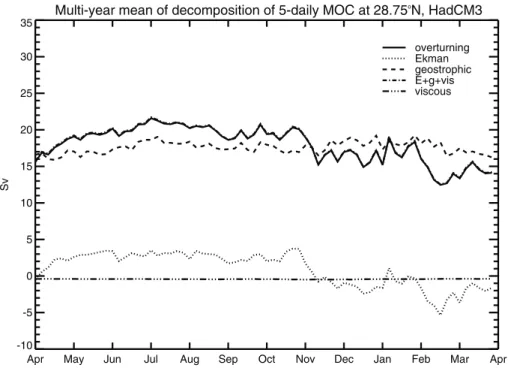
As an example, this decomposition is shown for HadCM3 in Fig. 2. In GENIE, we calculateTover, TEk and Tvis, and infer Tgeo as a residual. This model uses an annual climatology of windstress as a constant term, soTEk does not contribute to variability. In FORTE, we calculateTover,TEkandTvisdue to the Laplacian diffusion term, and infer

Tgeo as the residual. This means that the biharmonic diffusion term is included inTgeo.

5

This term is implicit in the model (Webb et al., 1998) and could not be calculated offline. It is relatively large and it is unclear how to interpret it physically. The components of transport could not be computed for FRUGAL and CHIME.

The mean and 5-day variability of the components of observed and simulated trans-ports are shown in Table 1. In the mean, the geostrophic term is largest in all cases.

10

The Ekman term is relatively small and positive, and the viscous term even smaller and negative, except in GENIE, in which the viscous (actually frictional) term is larger than in other models and the signs of these two terms are the other way round. As discussed above, the largest part of the variability is the mean annual cycle. The two main sources of this variability areTgeoandTEkin the models, as in observations (Cunningham et al.,

15

2007). However, Tgeo variability is smaller than TEk variability in models whereas in observations the reverse is true (Table 1). It is evident in Fig. 2 that the Ekman term dominates the annual cycle in HadCM3, for example. We find thatTgeovariability tends to be underestimated in models as compared to observations. This suggests that mod-els underestimate pressure anomalies along the eastern/western boundaries, possibly

20

as the result of underestimating the adiabatic upwelling/downwelling processes driven by alongshore wind-stress due to the coarse resolution which spreads the effect over one grid box instead of a more confined area in reality.

As in the observed variability (Cunningham et al., 2007), the externalText and inter-nalTint components ofTgeo in the upper 1000 m strongly anticorrelate in most models

25

(12)

OSD

8, 219–246, 2011

AMOC

Title Page

Tables Figures

◭ ◮

Back Close

Full Screen / Esc

Discussion

P

a

per

|

Dis

cussion

P

a

per

|

Discussion

P

a

per

|

Discussio

n

P

a

per

|

|d Tgeo/d t| ≪ |d Tint/d t|. The physical mechanism for the latter still requires further work

to be fully elucidated.

Variability due to the viscous termT_vis is small but not quite negligible. This term is not calculated for the observational array, because it represents the effect of unresolved motion and, by definition, any quantity measured by the array has been “resolved” by it.

5

The analogue of this term would be any contribution toToverfrom ageostrophic motion; the observational estimate assumes that the motion is geostrophic or Ekman, as it has to do because the current is not directly measured at all, except in the Florida Straits and near the western boundary.

5 Meridional coherence of transport and its components

10

On the assumption that the temporal variability of the circulation is coherent throughout the basin, a commonly used AMOC index from AOGCM results isM_max, the maximum of the overturning streamfunction, wherever it occurs, within a range of latitude and depth in the Atlantic, rather than at fixed latitude and depth. The RAPID/MOCHA array is intended to monitor the AMOC, by measuring the circulation at only one latitude. In

15

the model results we can investigate how wellMmaxandToverat 26 ◦

N representToverat other latitudes. GENIE is omitted from this analysis because it has no high-frequency or interannual variability, and CHIME and FRUGAL because all required timeseries are not available.

Calculated from 5-day means in the RAPID-models, the time-meanMmax is larger

20

than the transport at 26◦N, as it must be by construction, but the variability ofMmaxis generally less (Table 1). In annual means, however, the two timeseries have similar standard deviations. We have evaluated the same statistics from the AOGCMs of the Coupled Model Intercomparison Project Phase 3 (CMIP3), finding that in 16 out of 20 of them the annual standard deviation is similar inMmaxand at 26

◦

N (Table 2) (“similar”

25

when the difference between 2 standard deviations is less than 0.5 Sv); the exceptions are GISS-ER, GISS-AOM, INM-CM3.0 and IAP-FGOALS1.0g. That suggests greater

(13)

OSD

8, 219–246, 2011

AMOC

Title Page

Tables Figures

◭ ◮

Back Close

Full Screen / Esc

Discussion

P

a

per

|

Dis

cussion

P

a

per

|

Discussion

P

a

per

|

Discussio

n

P

a

per

|

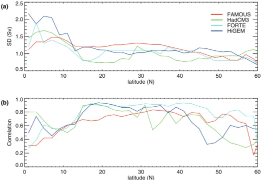
coherence across latitudes at longer time periods. However, only ten of the CMIP3 models and three of the RAPID-models have high correlation (exceeding 0.5) between the two timeseries. This is likely to be because there is a time lag between 26◦N and the latitudes ofMmax. Figure 3a shows the annual standard deviation of total transport as a function of latitude. No model has a well-defined maximum, but there is generally

5

more variability in the tropics, diminishing towards higher latitudes.

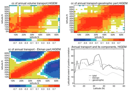
Next, we calculate the temporal correlation between different latitudes of timeseries of annual and 5-daily volume transports and their Ekman and geostrophic components, in HadCM3, FAMOUS, FORTE and HiGEM. Positive correlations are found between neighbouring latitudes in all timeseries, diminishing with increasing separation (eg.,

10

for annual timeseries in HiGEM, Fig. 4). Anticorrelation is found for widely spaced latitudes in the Ekman component. Since this component is wind-forced, the anticor-relation must indicate opposing signs of zonal windstress, occurring on opposite sides of the anomalies in atmospheric pressure and circulation that produce the windstress anomalies. It is notable that the anticorrelation is found for both 5-daily (figure not

15

shown) and annual data, even more pronounced in the former.

We define the “correlation length” as a function of latitude y to be the width of the range of latitudes whose timeseries which have a temporal correlation exceeding 0.5 with the timeseries at latitudey. Within 15–60◦N, the correlation lengths are typically 20–40◦in the annual timeseries (see Table 1 for 26◦N and Fig. 4 for HiGEM).

Correla-20

tion lengths are greater for the annual total and the geostrophic components than for the Ekman. They are also greater for annual total transports than for 5-daily total trans-ports, due to the greater coherence of the annual geostrophic component. Bingham et al. (2007, their Fig. 2c) also showed long-range coherence of annual total transport for HadCM3.

25

(14)

OSD

8, 219–246, 2011

AMOC

Title Page

Tables Figures

◭ ◮

Back Close

Full Screen / Esc

Discussion

P

a

per

|

Dis

cussion

P

a

per

|

Discussion

P

a

per

|

Discussio

n

P

a

per

|

ofToverat 26 ◦

N and 50◦N; only two models have a coe_fficient exceeding 0.5. Correla-tion is increased somewhat by including lags of a few years, but still does not exceed 0.5 in most cases. In models where there is a lag, variability ofToverat 50◦N precedes 26◦N, indicating that the forcing of the large-scale geostrophic variability comes from the north. A similar relation between AMOC at 26◦N and 50◦N with a time lag of 4

5

years is found in GFDL-CM2.1 (Zhang, 2010).

6 Relation of northward volume transport to heat transport

The climatic relevance of the AMOC arises from its association with the northward heat transport. This aspect is assessed by correlating the annual-mean time series of AMOC to that of the ocean heat transport (AOHT) at di_fferent latitudes (Fig. 5) in

10

the North Atlantic. This analysis can only be done for HadCM3, FAMOUS, FORTE, HiGEM and partly for CHIME. (AOHT is unavailable for other RAPID models and most of the CMIP3 models.) The time-mean heat transport is maximum around 10–30◦N, where it is about 1 PW (Fig. 6a, Table 1) in models. Compared to the observational estimate of Ganachaud and Wunsch (2003), HiGEM and FORTE values are within the

15

error bars of 2 of the 3 North Atlantic latitudes, while HadCM3 and CHIME are closer to the estimate around 50 N. FAMOUS heat transports are generally underestimated. LikeTover, AOHT does not have a well-defined maximum in variability as a function of latitude (Fig. 6b). Though the volume and heat transport variations in the models do not have a similar zonal profile, in general a good degree of temporal correlation is

20

found between them at all latitudes from 15◦N to 45◦N (Figs. 5, 3b, Table 1 for 26◦N). The slopes of the regression are fairly similar between 26–45◦N, indicating the positive volume-heat transport relationship at these latitudes. However, since the AMOC at 26◦N and 50◦N are not strongly correlated (Sect. 5), we expect that AOHT at 50◦N, in the latitudes of the Northern Europe, is not strongly correlated with the AMOC at 26◦N.

25

Indeed this is the case in HadCM3, FAMOUS, FORTE, CHIME and HiGEM (Table 1).

(15)

OSD

8, 219–246, 2011

AMOC

Title Page

Tables Figures

◭ ◮

Back Close

Full Screen / Esc

Discussion

P

a

per

|

Dis

cussion

P

a

per

|

Discussion

P

a

per

|

Discussio

n

P

a

per

|

7 Concluding remarks

We have shown that the 5-daily standard deviation of the AMOC simulated in the RAPID set of coupled climate models is comparable to that of the RAPID/MOCHA ob-servational estimate from the array at about 26◦N. This is an evaluation of a property that is unlikely to have been “tuned” during model development, because the

observa-5

tional estimate is new. Surprisingly, there is no systematic relation between the model resolution and the magnitude of variability. The standard deviation has contributions from high-frequency variability (timescale of a few days), the annual cycle and inter-annual variability. The models generally have more high-frequency variability than that estimated from observations, and a similar amplitude of annual cycle, but a spread in

10

simulating the shape of the cycle. The observational dataset (of 5 years) as yet is not long enough to assess simulated interannual variability. In the RAPID models and in most CMIP3 AOGCMs, the magnitude of interannual variability in the AMOC at 26◦N and in the maximum of the AMOC are similar, the latter being a commonly used model index.

15

We have dynamically decomposed the variability at about 29◦N (slightly north of the RAPID/MOCHA array in order to avoid complications with model coastlines) into Ek-man, geostrophic (i.e. due to pressure and sea-level gradient) and viscous/frictional components. The AMOC at 29◦N is predominantly geostrophic, but the Ekman term also contributes to variability. Ekman variability is more important in models than in

20

observations. Other ageostrophic terms contribute non-negligible variability in models, but are neglected in the observational estimate. Our study implies that such a de-composition of the transport is worth checking in the future intercomparison studies of AOGCMs in order to gain a better understanding of the processes responsible and the realism of their simulation.

25

(16)

OSD

8, 219–246, 2011

AMOC

Title Page

Tables Figures

◭ ◮

Back Close

Full Screen / Esc

Discussion

P

a

per

|

Dis

cussion

P

a

per

|

Discussion

P

a

per

|

Discussio

n

P

a

per

|

geostrophic coherence. But it does not extend over the whole basin (also found by Lozier et al., 2010). Consequently the AMOC at 26◦N does not have a high corre-lation with the AMOC or with heat transport at mid-to-high latitudes. Since the latter has a practical importance, and because this analysis, Zhang (2010) and Hodson and Sutton (2011) all suggest that AMOC variability on multiannual timescales propagates

5

from north to south, it would be useful to monitor the AMOC at higher latitudes as well as at 26◦N.

Acknowledgement. This study was supported by the “UK RAPID Thermohaline Circulation

Coupled Model Intercomparison Project” (UKTHCMIP) of the RAPID programme of the Nat-ural Environment Research Council, under grants NERC NE/C509366/1 and NE/C522268/1. 10

Data from UKTHCMIP are available from the British Atmospheric Data Centre. Data from the RAPID-WATCH MOC monitoring project are funded by the NERC and are available from www.noc.soton.ac.uk/rapidmoc. We acknowledge the CMIP3 modelling groups for making their model output available as, the Program for Climate Model Diagnosis and Intercomparison (PCMDI) for collecting and archiving this data, and the WCRP’s Working Group on Coupled 15

Modelling (WGCM) for organizing the model data analysis activity. The WCRP CMIP3 multi-model dataset is supported by the O_ffice of Science, US Department of Energy. Jonathan Gregory was partly supported by the Joint DECC and Defra Integrated Climate Programme, DECC/Defra (GA01101).

References 20

Baehr, J., Cunnningham, S., Haak, H., Heimbach, P., Kanzow, T., and Marotzke, J.: Observed and simulated estimates of the meridional overturning circulation at 26.5◦N in the Atlantic, Ocean Sci., 5, 575–589, doi:10.5194/os-5-575-2009, 2009.

Biastoch, A., B ¨oning, C. W., Getzla_ff, J., Molines, J.-M., and Madec, G.: Mechanisms of interannual-decadal variability in the meridional overturning circulation of the mid-latitude 25

North Atlantic Ocean, J. Climate, 21, 6599–6615, doi:10.1175/2008JCLI2404.1, 2008. Bigg, G. R. and Wadley, M. R.: Millennial changes in the oceans: an ocean modeller’s

view-point, J. Quaternary Sci., 16, 309–319, 2001.

(17)

OSD

8, 219–246, 2011

AMOC

Title Page

Tables Figures

◭ ◮

Back Close

Full Screen / Esc

Discussion

P

a

per

|

Dis

cussion

P

a

per

|

Discussion

P

a

per

|

Discussio

n

P

a

per

|

Bingham, R. J., Hughes, C. W., Roussenov, V., and Williams, R. G.: Meridional coherence of the North Atlantic meridional overturning circulation, Geophys. Res. Lett., 34, L23606, doi:10.1029/2007GL031731, 2007.

Blaker, A. T., Sinha, B., Wallace, C., Smith, R., and Hirschi, J. J.-M.: A description of the FORTE 2.0 coupled climate model, Geosci. Model Dev., in preparation, 2011.

5

Bleck, R.: An oceanic general circulation model framed in hybrid isopycnic-cartesian coordi-nates, Ocean Model., 4, 55–88, 2002.

Collins, M., Botzet, M., Carril, A. F., Drange, H., Jouzeau, A., Latif, M., Masina, S., Ot-teraa, O. H., Pohlmann, H., Sorteberg, A., Sutton, R. T., and Terray, L.: Interannual to decadal climate predictability in the North Atlantic: a multimodel-ensemble study, J. Climate, 10

19, 1195–1202, 2006.

Cunningham, S. A., Kanzow, T., Rayner, D., Baringer, M. O., Johns, W. E., Marotzke, J., Long-worth, H. R., Grant, E. M., Hirschi, J. J.-M., Beal, L. M., Meinen, C. S., and Bryden, H.: Tem-poral variability of the Atlantic meridional overturning circulation at 26.5◦N, Science, 317, 935–938, 2007.

15

Dong, B.-W. and Sutton, R. T.: The dominant mechanisms of variability in Atlantic Ocean heat transport in a coupled ocean-atmosphere GCM, Geophy. Res. Lett., 28, 2445–2448, 2001. Edwards, N. R. and Marsh, R.: Uncertainties due to transport-parameter sensitivity in an effi

-cient 3-D ocean climate model, Clim. Dynam., 24, 415–433, 2005.

Ganachaud, A. and Wunsch, C.: Large scale ocean heat and freshwater transports during the 20

World Ocean Circulation Experiment, J. Climate, 16, 696–705, 2003.

Gordon, C., Cooper, C., Senior, C. A., Banks, H., Gregory, J. M., Johns, T. C., Mitchell, J. F. B., and Wood, R. A.: The simulation of SST, sea ice extents and ocean heat transports in a version of the Hadley Centre coupled model without flux adjustments, Clim. Dynam., 16, 147–168, doi:10.1007/s003820050010, 2000.

25

Gregory, J. M., Dixon, K. W., Stouffer, R. J., Weaver, A. J., Driesschaert, E., Eby, M., Fichefet, T., Hasumi, H., Hu, A., Jungclaus, J. H., Kamenkovich, I. V., Levermann, A., Montoya, M., Mu-rakami, S., Nawrath, S., Oka, A., Sokolov, A. P., and Thorpe, R. B.: A model intercomparison of changes in the Atlantic thermohaline circulation in response to increasing atmospheric CO₂concentration, Geophys. Res. Lett., 32, L12703, doi:10.1029/2005GL023209, 2005. 30

Hodson, D. L. R. and Sutton, R. T.: The impact of model resolution on MOC adjustment in a coupled climate model, Clim. Dynam., in preparation, 2011.

(18)

OSD

8, 219–246, 2011

AMOC

Title Page

Tables Figures

◭ ◮

Back Close

Full Screen / Esc

Discussion

P

a

per

|

Dis

cussion

P

a

per

|

Discussion

P

a

per

|

Discussio

n

P

a

per

|

A monitoring design for the Atlantic meridional overturning circulation, Geophy. Res. Lett., 30, 1413, doi:10.1029/2002GL016776, 2003.

Jones, C., Gregory, J. M., Thorpe, R., Cox, P., Murphy, J., Sexton, D., and Valdes, P.: Systematic optimisation and climate simulations of FAMOUS, a fast version of HadCM3, Clim. Dynam., 25, 189–204, 2005.

5

Keenlyside, N. S., Latif, M., Jungclaus, J., Kornblueh, L., and Roeckner, E.: Advancing decadal-scale climate prediction in the North Atlantic sector, Nature, 453, 84–88, 2008.

Knight J. R., Allan, R. J., Folland, C. K., Vellinga, M., and Mann, M. E.: A signature of persistent natural thermohaline circulation cycles in observed climate, Geophys. Res. Lett., 32, L20708, doi:10.1029/2005GL024233, 2005.

10

Lozier, M. S., Roussenov, V., Reed, M. S. C., and Williams, R. G.: Opposing decadal changes for the North Atlantic meridional overturning circulation, Nature Geosci., 3, 728– 734, doi:10.1038/ngeo947, 2010.

Meehl, G. A., Stocker, T. F., Collins, W. D., Friedlingstein, P., Gaye, A. T., Gregory, J. M., Ki-toh, A., Knutti, R., Murphy, J. M., Noda, A., Raper, S. C. B., Watterson, I. G., Weaver, A. J., 15

and Zhao, Z.-C.: Global Climate Projections, Climate Change 2007: The Physical Science Basis, Contribution of Working Group I to the Fourth Assessment Report of the Intergovern-mental Panel on Climate Change, edited by: Solomon, S., Qin, D., Manning, M., Chen, Z., Marquis, M., Averyt, K. B., Tignor, M., and Miller, H. L., Cambridge University Press, Cam-bridge, UK and New York, NY, USA, 2007.

20

Megann, A. P., New, A. L., Blaker, A. T., and Sinha, B.: The sensitivity of a coupled climate model to its ocean component, J. Climate, 23, 5126–5150, 2010.

Pacanowski, R. C.: MOM 1 Documentation Users Guide and Reference Manual GFDL Ocean Technical Report, Geophysical Fluid Dynamics Laboratory, NOAA, Princeton, USA, 1990. Schmittner, A., Latif, M., and Schneider, B.: Model projections of the North Atlantic thermo-25

haline circulation for the 21st century assessed by observations, Geophys. Res. Lett., 32, L23710, doi:10.1029/2005GL024368, 2005.

Sha_ffrey, L. C., Stevens, I., Norton, W. A., Roberts, M. J., Vidale, P. L., Harle, J. D., Jrrar, A., Stevens, D. P., Woodage, M. J., Demory, M. E., Donners, J., Clark, D. B., Clayton, A., Cole, J. W., Wilson, S. S., Connolley, W. M., Davies, T. M., Iwi, A. M., Johns, T. C., King, J. C., 30

New, A. L., Slingo, J. M., Slingo, A., Steenman-Clark, L., and Martin, G. M.: UK-HiGEM: The new UK High Resolution Global Environment Model. Model description and basic evaluation, J. Climate, 22, 1861–1896, 2009.

(19)

OSD

8, 219–246, 2011

AMOC

Title Page

Tables Figures

◭ ◮

Back Close

Full Screen / Esc

Discussion

P

a

per

|

Dis

cussion

P

a

per

|

Discussion

P

a

per

|

Discussio

n

P

a

per

|

Smith, R., Osprey, A., and Gregory, J. M.: A description of the FAMOUS (version XDBUA) climate model and control run, Geosci. Model Dev., 1, 53–68, 2008.

Stouffer, R. J., Yin, J., Gregory, J. M., Dixon, K. W., Spelman, M. J., Hurlin, W., Weaver, A. J., Eby, M., Flato, G. M., Hasumi, H., Hu, A., Jungclaus, J. H., Kamenkovich, I. V., Lever-mann, A., Montoya, M., Murakami, S., Nawrath, S., Oka, A., Peltier, W. R., Robitaille, D. Y., 5

Sokolov, A., Vettoretti, G., and Webber, S. L.: Investigating the causes of the response of the thermohaline circulation to past and future climate changes, J. Climate, 19, 1365–1387, 2006.

Vellinga, M. and Wood, R. A.: Global climatic impacts of a collapse of the Atlantic thermohaline circulation, Clim. Change, 54, 251–267, 2002.

10

Weaver, A. J., Eby, M., Wiebe, E. C., Bitz, C. M., Duffy, P. B., Ewen, T. L., Fanning, A. F., Holland, M. M., MacFadyen, A., Matthews, H. D., Meissner, K. J., Saenko, O., Schmittner, A., Wang, H., and Yoshimori, M.: The UVic Earth System Climate Model: model description, climatology and application to past, present and future climates, Atmos.-Ocean, 39, 361– 428, 2001.

15

Webb, D. J.: An ocean model code for array processor computers, Comput. Geosci., 22, 569– 578, 1996.

Webb, D. J., de Cuevas, B. A., and Richmond, C. S.: Improved advection schemes for ocean models, J. Atmos. Ocean. Technol., 15, 1171–1187, 1998.

Zhang, R.: Latitudinal dependence of Atlantic meridional overturning circulation (AMOC) vari-20

(20)

OSD

8, 219–246, 2011

AMOC

Title Page

Tables Figures

◭ ◮

Back Close

Full Screen / Esc

Discussion

P

a

per

|

Dis

cussion

P

a

per

|

Discussion

P

a

per

|

Discussio

n

P

a

per

|

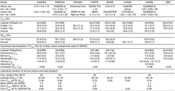
Table 1. Specifications of the RAPID-models; time-mean and standard deviations (X(Y) indi-catesX is mean andY is SD) of simulated Atlantic ocean meridional overturning transport (in Sv),T_over, at 26◦N and of the maximum of Atlantic MOC,M_maxon 5-daily and annual timescales; time-mean and standard deviation (SD) of the simulated 5-dailyT_over, 29◦N and its decomposed components (T_Ek: Ekman part,T_geo: geostrophic part,T_vis: viscous/frictional part andT_adv: ad-vection part); time-mean of simulated annual ocean meridional heat transport (AOHT in PW), 26◦N and the interannual correlationT_overat 26◦N withM_max, AOHT at 26◦N and AOHT at 50◦N. The RAPID/MOCHA observational estimate (of 5 years) is given in the last column. In HiGEM and FORTE, the transport component due to viscous part has 2 parts namely, by the laplacian and biharmonic terms. In FORTE, the biharmonic term is implicit and could not be calculated offline. The FRUGAL transport at 26◦N is calculated along a curvilinear gridline which is near 26◦N. Time-step data is used in GENIE which has an ocean time-step of 3.65 days. GENIE has no seasonal variability in wind-stress and no interannual variability. Meridional correlation length (in◦lat) at 26◦N is defined as the latitudinal extent of positive correlation above 0.5 in both directions. FRUGAL and CHIME data are only available for some of the calculations.

Model HadCM3 FAMOUS FRUGAL FORTE GENIE CHIME HiGEM OBS

Atmos res: 3.75×2.5×19 HadCM3 at Enhanced UVic IGCM3 T42 UVic 2-D HadCM3 HadGEMI at

lon×lat×level 7.5×3.75×11 ×15 atmos 1.25×0.83×38

Ocean res: 1.25×1.25×20 HadCM3 at MOM V2 with MOM GOLDSTEIN HYCOM at HadGEMI at

lon×lat×level 3.75×2.5×20 high-res Arctic 2×2×15 10×5×8 1.25×1.25×25 0.33×0.33×40

Tover(Sv)

Latitude◦N/Depth (m) 26.3/995 26.3/995 26.0/1365 26.4/1158 26.3/1050 26.9/959 26.5/1041

5-daily, 1 yr 19.2 (4.2) 18.9 (4.2) 26.4 (1.3) 16.3 (4.2) 16.4 (0.3) 15.2 (3.8) 15.1 (2.7) 20.5 (4.1)

5-daily, 10 yr 17.1 (4.1) 18.2 (4.2) 26.4 (1.4) 17.2 (4.5) 16.4 (0.3) 15.0 (3.3) 15.5 (4.0) 18.6 (4.5)

Annual 16.8 (0.9) 20.6 (1.3) 17.6 (1.1) 16.5 (0) 18.8 (1.2) 16.4 (1.0)

Mmax(Sv)

5 d–10 yrs 21.9 (2.4) 18.7 (3.0) 26.5 (1.3) 21.3 (2.5) 18.5 (0.3) 20.6 (2.5)

Annual 18.9 (0.7) 20.0 (1.3) 19.8 (1.1) 18.6 (0) 20.1 (1.7) 18.9 (1.1)

Dynamical decomposition ofTover(Sv) for 5-daily means (except time-step for GENIE)

Latitude◦N/Depth(m) 28.8/995 28.8/995 30/1365 30/1158 28.9/959 26.5/1041

OverturningTover 18.0 (4.3) 18.1 (3.7) 16.5 (3.9) 16.1 (0.12) 15.7 (3.6) 18.6 (4.5)

EkmanTEk 0.9 (4.0) 3.5 (3.5) 1.4 (3.8) −2.3 (0) 1.6 (3.3) 3.6 (3.2)

GeostrophicTgeo 17.6 (2.3) 15.3 (1.6) 15.2 (2.8) 16.8 (0.1) 14.4 (2.6) 15.0 (3.5)

ViscousTvis −0.4 (0.1) −0.8 (0.2) −0.1(0.1) 1.7 (0.02) −0.2 (0.0),−0.1 (0.1)

AdvectiveTadv 0.3 (0.6)

Correlation (Tint,Text) −0.98 −0.94 −0.64 −0.96 −0.83

Latitudinal variation of annual volume and heat transport

Corr. length (◦_{lat), 26}◦_N ₄₀ ₂₄ ₂₅ ₂₈

Latitude ofMmax(◦N) 35–45 31–34 30–40 46–51 23–60 34–45

Corr (Tover26

◦

N,Mmax) 0.38 0.96 0.70 0.93 0.53 0.74

Mean AOHT, 26◦N(PW) 1.0 0.8 1.1 1.1

Corr (Tover, AOHT), 26

◦

N 0.8 0.8 0.9 0.9

Corr (Tover26

◦

N, AOHT50◦N) 0.00 0.24 0.39 0.42 0.36

(21)

OSD

8, 219–246, 2011

AMOC

Title Page

Tables Figures

◭ ◮

Back Close

Full Screen / Esc

Discussion

P

a

per

|

Dis

cussion

P

a

per

|

Discussion

P

a

per

|

Discussio

n

P

a

per

|

Table 2.Comparison of standard deviations (in Sv) of Atlantic MOC (T_over) at 26◦N, 50◦N and of the maximum of Atlantic MOC,Mmax, and their correlations in the CMIP3 models. Linear

or quadratic trend is removed for unsteady runs before the calculation. The lag betweenTover

at 26◦N and 50◦N is shown which gives the largest correlation of their timeseries. The lag is negative whenTover26◦N lags.

Model SD SD Corr SD Corr Lag Lagged corr.

Mmax Tover (Tover26◦N, Tover (Tover26◦N, (years) (Tover26◦N,

26◦N M_max) 50◦N T_over50◦N) T_over50◦N)

CSIRO-Mk3.0 1.8 1.6 0.85 1.6 0.53 −1 0.70

CNRM-CM3 1.8 2.1 0.20 1.7 0.05 −2 0.41

CCCMA-CGCM3.1(T63) 0.72 0.71 0.85 0.67 0.11 −1 0.51

CCCMA-CGCM3.1(T47) 0.50 0.63 0.09 0.65 −0.14 −2 0.39

BCCR-BCM2-0 0.93 0.91 0.61 0.82 −0.02 −2 0.25

GISS-ER 2.7 0.97 0.06 2 0.35 −1 0.48

GISS-AOM 7.2 1.5 0.01 2.0 0.19 −3 0.44

GFDL-CM2.1 1.3 1.2 0.39 1.1 −0.01 −5 0.46

GFDL-CM2.0 1.1 1.1 0.38 1.1 0.12 −2 0.51

CSIRO-Mk3.5 1.2 1.0 0.88 1.4 0.52 −1 0.72

MIROC3.2 (hires) 0.8 1.0 0.16 0.82 0.02 −1 0.28

INM-CM3.0 2.9 3.4 0.47 1.7 0.07 −2 0.52

INGV-ECHAM4 1.6 1.9 0.61 1.5 0.09 −3 0.58

IAP-FGOALS1.0g 2.3 0.49 0.09 0.43 −0.26 10 −0.02

NCAR-CCSM3.0 1.8 1.2 0.88 1.1 0.24 −2 0.45

MRI-CGCM2.3.2a 0.71 0.73 0.53 0.97 −0.23 −1 0.34

MIUB-ECHOG 1.3 1.0 0.35 1.2 0.23 −4 0.53

MIROC3.2 (medres) 0.72 0.64 0.67 0.69 0.07 −2 0.44

UKMO-HadGEM1 1.0 1.0 0.68 0.77 0.05 −1 0.21

(22)

OSD

8, 219–246, 2011

AMOC

Title Page

Tables Figures

◭ ◮

Back Close

Full Screen / Esc

Discussion

P

a

per

|

Dis

cussion

P

a

per

|

Discussion

P

a

per

|

Discussio

n

P

a

per

|

(a)5-daily time series – a single year (b)5-daily time series – 10-year mean

5-daily Atlantic MOC at 26N for a year- Control

Apr May Jun Jul Aug Sep Oct Nov Dec Jan Feb Mar 0

5 10 15 20 25 30

Sv

FAMOUS HadCM3 FORTE HiGEM CHIME GENIE FRUGAL OBS

Multi-year mean of 5-daily Atlantic MOC at 26N - Control

May Jun Jul Aug Sep Oct Nov Dec Jan Feb Mar Apr 5

10 15 20 25 30

Sv

FAMOUS HadCM3 FORTE HiGEM CHIME GENIE FRUGAL OBS

Fig. 1. Atlantic MOC (T_over) at 26◦N(a)5-daily time series – for a single year(b)5-daily time series – 10-year mean in models and 5-year mean in observations (The FRUGAL transport is calculated along a curvilinear gridline which is near 26◦N. For GENIE, time-step data is plotted; its ocean time-step is 3.65 days)(c)5-daily – power spectrum (note the logarithmic scale on they-axis. Oscillations of less than 40-day period are significant in observations and in all the models, except FRUGAL and GENIE), and(d)annual time series (HiGEM data is only 90 years long after the spin-up time).

(23)

OSD

8, 219–246, 2011

AMOC

Title Page

Tables Figures

◭ ◮

Back Close

Full Screen / Esc

Discussion

P

a

per

|

Dis

cussion

P

a

per

|

Discussion

P

a

per

|

Discussio

n

P

a

per

|

(c)5-daily – power spectrum (d)Annual time series

Power spectrum of 5-daily AMOC at 26N

10 40 100 590

Period (days) 1

10 100 1000 2000 3000

Power spectral density (Sv

2 yr)

FAMOUS HadCM3 FORTE HiGEM CHIME OBS

1 year

Annual Atlantic MOC at 26N - Control

10 20 30 40 50 60 70 80 90 100

Years 12

16 20 24

Sv

FAMOUS HadCM3 FORTE HiGEM CHIME

(24)

OSD

8, 219–246, 2011

AMOC

Title Page

Tables Figures

◭ ◮

Back Close

Full Screen / Esc

Discussion

P

a

per

|

Dis

cussion

P

a

per

|

Discussion

P

a

per

|

Discussio

n

P

a

per

|

Multi-year mean of decomposition of 5-daily MOC at 28.75o_{N, HadCM3}

Apr May Jun Jul Aug Sep Oct Nov Dec Jan Feb Mar Apr

-10 -5 0 5 10 15 20 25 30 35

Sv

overturning Ekman geostrophic E+g+vis viscous

Fig. 2.Decomposition of 5-daily Atlantic MOC (T_over) into physical components at about 29◦N in HadCM3. The sum E+g+vis (dash-dotted) is almost coincident with the total overturning (solid).

(25)

OSD

8, 219–246, 2011

AMOC

Title Page

Tables Figures

◭ ◮

Back Close

Full Screen / Esc

Discussion

P

a

per

|

Dis

cussion

P

a

per

|

Discussion

P

a

per

|

Discussio

n

P

a

per

|

(a)

(b)

0 10 20 30 40 50 60

latitude (N) 0.5

1.0 1.5 2.0 2.5

SD (Sv)

FAMOUS HadCM3 FORTE HiGEM

0 10 20 30 40 50 60

latitude (N) 0.0

0.2 0.4 0.6 0.8 1.0

Correlation

Fig. 3.Zonal profile of(a)annual ocean meridional overturning transport (Tover) variability (Sv)

(26)

OSD

8, 219–246, 2011

AMOC

Title Page

Tables Figures

◭ ◮

Back Close

Full Screen / Esc

Discussion

P

a

per

|

Dis

cussion

P

a

per

|

Discussion

P

a

per

|

Discussio

n

P

a

per

|

10N 20N 30N 40N 50N 60N latitude,N

5N 10N 15N 20N 25N 30N 35N 40N 45N 50N 55N 60N

latitude,N

cc of annual volume transport,HiGEM

-0.7 -0.5 -0.3 -0.1 0.1 0.3 0.5 0.7

5N 10N 15N 20N 25N 30N 35N 40N 45N 50N 55N 60N

latitude,N

cc of annual transport-geostrophic part,HiGEM

-0.7 -0.5 -0.3 -0.1 0.1 0.3 0.5 0.7

10N 15N 20N 25N 30N 35N 40N 45N 50N 55N 60N

latitude,N

cc of annual transport - Ekman part,HiGEM

-0.7 -0.5 -0.3 -0.1 0.1 0.3 0.5 0.7

Annual transport and its components, HiGEM

10 20 30 40 50 60 Latitude (N)

0 10 20 30 40 50

Latitudinal extent of positive correlation

total Ekman geostrophic

Fig. 4.Cross-correlation of annual ocean meridional overturning transport,T_over(top left) and its physical components – geostrophic,Tgeo(top right), Ekman,Tek(bottom left) between latitudes

in the North Atlantic in HiGEM and their meridional correlation length (bottom right). Correlation length (◦lat) as a function of latitudey is defined as the width of the range of latitudes whose timeseries which have a temporal correlation exceeding 0.5 with the timeseries at latitudey.

(27)

OSD

8, 219–246, 2011

AMOC

Title Page

Tables Figures

◭ ◮

Back Close

Full Screen / Esc

Discussion

P

a

per

|

Dis

cussion

P

a

per

|

Discussion

P

a

per

|

Discussio

n

P

a

per

|

Annual AOHT Vs. AMOC at 26N

10 12 14 16 18 20 22 24

AMOC (Sv) 0.2

0.6 1.0 1.4

AOHT (PW)

FAMOUS (0.76, 0.04) HadCM3 (0.84, 0.06) FORTE (0.89, 0.06) HiGEM (0.87, 0.06)

10 12 14 16 18 20 22 24

AMOC (Sv) 0.2

0.6 1.0 1.4

AOHT (PW)

10 12 14 16 18 20 22 24

AMOC (Sv) 0.2

0.6 1.0 1.4

AOHT (PW)

10 12 14 16 18 20 22 24

AMOC (Sv) 0.2

0.6 1.0 1.4

AOHT (PW)

10 12 14 16 18 20 22 24

AMOC (Sv) 0.2

0.6 1.0 1.4

AOHT (PW)

10 12 14 16 18 20 22 24

AMOC (Sv) 0.2

0.6 1.0 1.4

AOHT (PW)

(28)

OSD

8, 219–246, 2011

AMOC

Title Page

Tables Figures

◭ ◮

Back Close

Full Screen / Esc

Discussion

P

a

per

|

Dis

cussion

P

a

per

|

Discussion

P

a

per

|

Discussio

n

P

a

per

|

(a)

(b)

0 10 20 30 40 50 60

latitude (N) 0.0

0.4 0.8 1.2 1.6

Mean (PW)

0 10 20 30 40 50 60

latitude (N) 0.00

0.02 0.04 0.06 0.08 0.10

SD (PW)

FAMOUS HadCM3 FORTE HiGEM OBS CHIME

Fig. 6.Zonal profile of(a)mean annual ocean meridional heat transport (PW) and(b)variability of annual ocean meridional heat transport in the North Atlantic. The observational estimate of heat transport is from Ganachaud and Wunsch (2003). CHIME data is only available in 10◦ latitude intervals.