Mean vertical wind in the mesosphere-lower thermosphere region
(80±120 km) deduced from the WINDII observations
on board UARS
V. Fauliot1, G. Thuillier1, F. Vial2
1
Service d¢AeÂronomie du CNRS, Bp 3, F-91 371 VerrieÁres le Buisson, France 2
Laboratoire de MeteÂorologie Dynamique du CNRS, Ecole Polytechnique, F-91128 Palaiseau, France
Received: 15 November 1996 / Revised: 24 February 1997 / Accepted 25 February 1997
Abstract.The WINDII interferometer placed on board the Upper Atmosphere Research Satellite measures temperature and wind from the O(1S) green-line emis-sion in the Earth's mesosphere and lower thermosphere. It is a remote-sensing instrument providing the hori-zontal wind components. In this study, the vertical winds are derived using the continuity equation. Mean wind annually averaged at equinoxes and solstices is shown. Ascendance and subsidence to the order of 1±2 cm s)1present a seasonal occurrence at the equator
and tropics. Zonal Coriolis acceleration and adiabatic heating and cooling rate associated to the mean meri-dional and vertical circulations are evaluated. The line emission rate measured together with the horizontal wind shows structures in altitude and latitude correlated with the meridional and vertical wind patterns. The eect of wind advection is discussed.
1 Introduction
Prior to the launch of the Upper Atmosphere Research Satellite (UARS), information on the wind systems in the mesosphere and lower thermosphere (hereafter referred to as the MLT region) mainly came from radar observations made at single locations. With few excep-tions (e.g. Meek and Manson, 1989), vertical winds are not documented with such systems due to the diculties linked to their measurement (Reid, 1987). In particular, it is necessary to use an untilted vertically pointing radar beam, since otherwise the projection of the horizontal winds can lead to a contamination of the vertical wind estimate. In the MLT region, the vertical wind being of the order of few cm s)1 explains that except for the
thermosphere in the auroral zone, optical methods are not able to provide vertical wind measurements. Nev-ertheless, the knowledge of the vertical wind can lead to an improved understanding of the dynamical state of the
MLT region as illustrated, for example, by Coy et al.
(1986) in their discussion of the observations of Basley and Riddle (1984).
At ®rst order, the dynamical state of the MLT region is dominated by the acceleration of the mean ¯ow induced by dissipation of a dierent type of waves generated at lower altitudes, according to the Eliassen-Palm theorem. This acceleration is associated with an oppositely directed Coriolis force due to the meridional ¯ow generated by hydrostatic and geostrophic equilib-ria. By continuity, vertical motion is also generated which provides subsidence heating and adiabatic cool-ing. Thus the knowledge of meridional and vertical winds provides information on the momentum forcing and heating of the MLT region.
A method to deduce vertical wind was originally proposed by Ebel (1974) and later used by Miyahara
et al.(1991) and Portnyaginet al.(1995). Using most of the available radar data, they constructed an empirical model for the meridional mean winds in the MLT region. Then, using the continuity equation, they deduced the associated vertical mean winds. Using this empirical model, Miyaharaet al.(1991) and Portnyagin
et al. (1995) have shown that the knowledge of vertical and meridional mean winds allows one to estimate the mean momentum balance, adiabatic cooling and heat-ing, and provide new information on their latitudinal distribution and role in this region.
Although the approach used by Miyahara et al.
In addition to their role in the momentum and energy balance of the MLT region, mean vertical winds also play a role in the compositional structure of this region, as they transport vertically minor constituents. This should induce a signature in the airglow emissions occuring in the MLT region. Some of these minor constituents are also important absorbents of solar radiation and their transport can modify the energetic equilibrium of this region. As WINDII also provides intensity of several airglow emissions, it provides an interesting opportunity to explore the role played by mean horizontal and vertical motions in the observed distribution of these airglow emissions. This is the case of the O(1S) green-line emission at 557.7 nm, observa-tions from which the horizontal winds are deduced. Notice however that these two sets of data can be considered as independent.
The plan of this paper is as follows. In Sect. 2, the WINDII data base and the method of analysis used to deduce meridional and vertical mean winds are present-ed. In Sect. 3, we report some of our results for the meridional and vertical winds. The characteristics and variations with altitude and latitude of the O(1S) emission will be also presented. Section 4 is dedicated to the green-line intensity calculation. In Sect. 5, our results will be discussed and compared to those obtained by Miyaharaet al. (1991) and Portnyaginet al.(1995). We also present the momentum and energy sources deduced from the wind ®elds. We shall also explain the role played by mean meridional and vertical winds in the observed airglow latitude-height distribution. Finally, conclusions will be presented in Sect. 6.
2 Data base and analysis
2.1 The WINDII observations
WINDII, placed on board UARS, measures vertical pro®les of horizontal wind velocity, Doppler tempera-ture and line intensity from 75 to 300 km using several airglow emissions. The WINDII objectives and the instrument are described in detail by Shepherd et al.
(1993). Some information is given in the following, allowing a better understanding of the present study.
The WINDII wind-measurement principle consists in observing the Doppler shift of a natural emission line of the Earth's atmosphere airglow. This is achieved by use of a Michelson interferometer. By changing the inter-ferometer optical path dierence step by step, an interferogram of the chosen line is generated. Its phase shift with respect to the zero wind reference allows the derivation of the wind velocity along the line of sight. The reference phase is obtained from ground and on-board calibration measurements. The measurements are obtained in two vertical planes at 45 and 135 arc degrees from the spacecraft velocity vector. The measurements made at about 6-min time-dierence correspond to observations of the same volume of atmosphere under angles of about 90 arc degrees dierence. The combi-nation of these measurements allows us to obtain the
meridional and zonal wind components. Vertical pro-®les of zonal and meridional wind components as a function of latitude, longitude and time constitute the basic data set.
The data used in the present study are obtained by observation of the atomic oxygen emission line at 557.7 nm, providing information from 80 to 200 km in the daytime and 80 to 110 km during night-time. Wind accuracy depends upon several parameters, such as shot noise, spacecraft attitude and accuracy of the calibration data. It is estimated for individual measurement around 10±15 m s)1.
2.2 The WINDII data base
As already explained, the two ®elds of view of the WINDII instrument allows us to observe at angles of 45° and 135° to the spacecraft velocity vector. As the
two lines of view are on the same side of the orbital plan, the latitudinal coverage has a hemispheric asymmetry and ranges from 72°in one hemisphere to 42°latitude in
the other. Due to the orbital precession, the spacecraft yaws about every 36 days (henceforth referred to as a UARS month). Consequently, the latitudinal range of observation is also reversed from one hemisphere to the other leading to extend measurements between 72°S and
72°N.
The satellite crosses the same latitude circle at two distinct local times per orbit and completes 15 orbits per day. The orbital precession changes the local-time coverage by 20 min per day only. Thus, 36 days are required in order to cover 24 h local time in the 42
latitudinal range, while 72 days are necessary above it. In addition, it should be pointed out that the green-line emission is observed twice and four times per week during night-time and daytime, respectively. However, several continuous measurements over about 15 days also took place within the framework of the validation (Gaultet al., 1996; Thuillieret al., 1996). Despite these opportunities, the local-time coverage does not generally exceed 14 h per UARS month. The magnitude of the green-line emission rate imposes the vertical range of observations through the signal-to-noise ratio. The vertical extent of the region of production of the green-line emission varies signi®cantly from daytime to night-time conditions as a result of the dierent excita-tion processes involved in the creaexcita-tion of the (1S) state. Thus, the domain of the available measurements extends between 80±110 km at night and 80±200 km during the day. The height resolution of WINDII is of 3 km in the MLT region.
Given the temporal and spatial coverage of the data base, we adopt a binning so that mean and time-dependent regimes of the circulation can be character-ised with an acceptable noise/resolution compromise. The data base includes 27 months of observations from January 1992 to March 1994. Assuming no interannual variability, data are sorted into months and combined to construct a reference year. Data handling primarily consists in gathering measurements in boxes of 5°
latitude, 3 km height and 1 h local time. Thus, a zonal average is performed ensuring a globally coherent structure of the circulation. The inclination and preces-sion of the UARS orbit induce a coupling between local time and seasonal variations of the observed quantities. As already mentioned, for WINDII the expected local-time coverage of 24 h in 36 days is not achieved when using O(1S) observations only. However, we need a reliable local-time coverage properly to describe the dierent components of the wind system. The spatial and time averaging which result from the chosen binning reduce the random noise of measurements and the eects of the natural variability of atmospheric quanti-ties. In that condition, a 18-h local-time coverage is adequate to extract solar harmonics and prevailing components. This is achieved between 60 of latitude
by gathering 2 months of data from the reference year, but this implies that the sampling rate of the seasonal variation is reduced accordingly. Figure 1 presents the day-local time and day-latitude distribution for the reference year. The UARS yaw signature is clearly noticeable in Fig. 1b. Figure 1 also shows that using 2 months of data is adequate for the study we want to carry out.
It should be noted that the present organisation of the data removes the possible contribution of migrating planetary waves whose period varies from 2 days up to several weeks. The next step of the present study has to take into account the eect of the seasonal changes of tides and mean circulation characteristics on the local-time variations of the wind, since 2 months of data are combined. This last point will be carefully discussed in the next section, as it aects the validity of derived results.
2.3 Method for data analysis
As known, zonal mean wind strongly aects the structure of tides. For example, at mid-latitudes in the MLT region, the semi-diurnal tide experiences a rapid transition around equinoxes connected with the reversal of the zonal mean wind regime. This takes place within less than 1 month. Thus, tides and background winds may vary over time-scales shorter than the interval required to cover 24 h of local time. The seasonal evolution of the wind ®eld during this interval aliases into tidal components. Consequently, Fourier analysis (hereafter referred to as Method 1) directly applied to the hourly binned data would result in incorrect amplitude and phase of tides and magnitude of mean wind. Forbeset al. (1997) addressed this issue from an
empirical point of view. Based on the following statements:
1. space-based determinations of the zonal mean com-ponents usually represent faithful reproductions of the true results,
2. the mean component aliases into the tides much more than the tides alias into the mean,
they propose a method to seperate mean and tidal components. It consists in making a ®rst estimate of the mean component by averaging data over each 24-h local-time-interval. Assuming statement (1), the mean obtained in this way is at ®rst order an acceptable approximation of the true one. A new data set is constructed by removing this mean component from each original piece of data. This subtraction leads to smear out aliasing contribution of mean into tides which is dominant according to statement (2). Consequently, harmonic analysis applied to the new data set allows to obtain a realistic estimate of tidal components.
From this original work, we propose a method which takes into account the local-time sampling of our data base. Firstly, for each 2-month interval, mean and tidal components are extracted through least-squares ®t in terms of mean, semi-diurnal and diurnal components. Then, they are analysed in terms of mean, annual, semiannual and terannual components using a sliding 2-month window over the reference year. Thirdly as statement (2) is not necessarily valid when tidal
components are larger than mean winds, we remove ®rst either the mean wind or tides according to their relative amplitudes. This is achieved by subtracting from each original individual measurement its estimate obtained from the two preceding steps. These three steps are iteratively performed until the residues are smaller than 0.5 m s)1.
This procedure converges in less than three iterations. In addition, it takes into account the quick transitions such as those observed at equinoxes which occur within 1 month. This method will be referred to as Method 2. Using the Horizontal Wind Model predictions (He-dinet al., 1993), we built a data base using the WINDII sampling (latitude, local time and day) in order to test Method 2. We consider the zonal and meridional mean winds and the diurnal tide components at 40°N and
99-km altitude. For the zonal component, the amplitude of the seasonal variation of the mean wind is more important than that of the diurnal tide. For the meridional wind, there is the opposite situation with a dominant seasonal amplitude of the diurnal tide with respect to the mean wind. We apply Methods 1 and 2 to these simulated data sets. The two cases are illustrated in Fig. 2. We note that the largest component is always correctly retrieved by both methods. By applying Method 1, the weakest component contains signi®cant
aliasing eects. This weak component is only correctly retrieved when applying Method 2. Note that we shall use the mean meridional wind in this study which is weak with respect to the tidal component. This is why it is important to demonstrate that Method 2 allows the correct retrieval of the mean meridional wind.
2.4 Derivation of the mean vertical wind
Using the mean meridional circulation previously ex-tracted from the WINDII reference year, the vertical wind regime in the MLT region is derived from the continuity equation:
1
rcosu
@ @u v
cosu @w
@zÿw
1
H 1
@H @z
0;
whereris the radius of the Earth,uis the latitude,His
the scale height and v and w are the mean meridional and vertical winds, respectively.
An upper boundary condition is set as follows:
@w
@z 0 at z120 km:
Yet, its eect is negligible below 114 km. The scale height is estimated using the MSIS90 predictions.
3 Results
3.1 Mean meridional wind
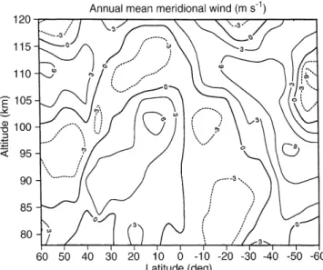
The data-base organisation as explained in Sect. 2.2 allows to calculate the annual mean of the meridional wind component. The results are shown in Fig. 3, which presents mean wind in metres per second. This ®gures shows a latitude-height cell organisation with northward and southward winds. Between 40° and 60°N, a
north-ward wind centred at 110-km altitude is associated with a similar southward wind centred at 95 km. A similar situation is shown in the 40°±60°S region with southward
winds at 110 km and northward winds at 95 km. At 10°N and 100 km, northward winds are present and
can be associated with southward winds in the other
hemisphere. Figure 3 shows an annual mean wind organised in cells reaching a typical velocity of 3 m s)1
and having an anti-symmetrical structure in latitude. Figures 4 and 5 present the mean meridional winds in October and January, respectively. In October, between 35°S and 35°N, winds present a distribution with
latitude rather symmetrical below 100 km and anti-symmetrical above. The anti-anti-symmetrical is found again above 40°. In January, winds remain northward below
105 km and southward above. These features are consistent with those obtained in April and July.
3.2 Mean vertical wind
Vertical winds are derived using the algorithms present-ed in Sect. 2.3, Fig. 6 shows the mean annual vertical
Fig. 3.Latitude-height distribution of the annual mean meridional wind (positive northward)
Fig. 4.Latitude-height distribution of the mean meridional wind in October
Fig. 5.Latitude-height distribution of the mean meridional wind in January
winds. The mean vertical wind velocity is of the order of 2 cm s)1. An ascendance at the equator is shown around
95±100 km and a subsidence at higher altitude. Com-paring the northern and the southern latitudes, a remarkable symmetry is noticeable with a subsidence at 85±90 km located at 40°S and N and two tropical
ascendances centred at 110±115 km.
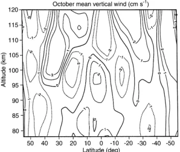
Figure 7 presents the mean vertical wind in October. An ascendance at the equator is located at 95±100 km and a subsidence above. The global wind pattern is symmetrical. Similar features are observed in April. Figure 8 presents wind patterns close to solstice. An ascendance is placed around 95±100 km, close to the equator, but shifted in the winter hemisphere and an anti-symmetrical structure is also shown at lower altitudes. These features are consistent with the results of July.
3.3 Mean green-line emission rate
The WINDII instrument is providing the simultaneous measurements of wind velocity and emission line intensity. Both are obtained as a function of altitude. The winds and green-line emission-rate pro®les have been similarly organised, the latter allowing to generate emission rates as a function of altitude and latitude.
During daytime, excitation processes are dominated by photo-dissociation. In order to extract the contribu-tion due only to dynamics, we use night-time data. The mean is separated from the tidal contribution by adjusting data to a mean with a semi-diurnal and diurnal term by a least-squares ®t. Using only night-time period data makes the extraction of mean and solar harmonic terms subject to aliasing. To validate our extraction algorithm, we made several simulations focusing on the eect of the lack of local-time coverage and presence of random noise upon the resulting estimate. The low noise aecting the green-line data emission rate allows us to retrieve the mean and both tidal terms within a few percent of error for a local-time coverage as small as 7 h.
Figure 9 shows the annual mean emission rate in photons cm)3s)1. The maximum emission rates in both
hemispheres are close to 120 photons cm)3s)1 and
located around 30°. Both maxima occur at an altitude
of 95±96 km. The emission-rate distribution is quasi-symmetrical around the equator as well as the layer shape, which varies as a function of latitude. The green-line layer presents a width (as de®ned at half maximum emission rate) which increases from 10 km at 40° to
12 km at the equator, where the emission rate is the lowest.
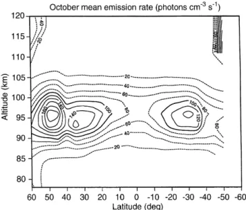
Similar to Fig. 9, Fig. 10 displays the emission-rate distribution in October. With respect to the annual mean, the maximum emission rate reaches 120±140 pho-tons cm)3s)1, the greatest intensity being observed in
Fig. 7. Latitude-height distribution of the mean vertical wind in October
Fig. 8. Latitude-height distribution of the mean vertical wind in January
the northern hemisphere. As for the annual mean, Fig. 10 also shows a quasi-symmetry with a layer width increasing from the mid-latitudes to the equator. We notice around 50° and above an emission-rate increase
around 95-km altitude and above, which is the bottom part of the green-line thermospheric emission pro®le. At these latitudes, the green-line emission is mainly gener-ated by precipitations of electrons in the auroral zone. Consequently, these features will be not considered in the present study.
Figure 11 presents the emission-rate distribution in January. The maximum emission rate stays around 95± 96 km and appears as a very stable feature independent of the season. The greatest line emission rate is observed in the summer hemisphere. As for Fig. 10, the auroral zone emission is also present. The absence of data in the southern hemisphere is due to the lighting conditions. At
equinoxes and solstices, the emission rate remains quasi-symmetrical with respect to the equator, which is the region of the lowest emission rate, while maxima occurs near the mid-latitudes.
4 Calculation of the green-line emission rate
A close inspection of Figs. 9±11 suggests that the latitudinal distribution of the mean emission rate of the green line is correlated to the mean wind system at the corresponding period. It is not surprising that winds modify the 557.7-nm intensity as they transport atomic oxygen and other consituents involved in its production as shown, for example in the case of tides, by Petitdidier and Teitelbaum (1979). Using the MSIS90 predictions, intensity of the green line will be calculated and compared with the WINDII observations (intensity and winds patterns).
4.1 The green-line emission
The green line is emitted by radiative de-excitation of the atomic oxygen in the (1S) state. O is mainly produced by photodissociation of O2. The loss of
atomic oxygen in the MLT region is primarily through a three-body recombination process with N2as the third
body. It is now admitted that the Barth's mechanism is responsible of the excitation of atomic oxygen and thus the green-line emission. This is a two-step mechanism:
OOM!O2M O2O!O 1S O2
Thus, the green-line intensity depends not only on the production and loss of atomic oxygen but also of the quenching of O2 (through collisions with M or O) and O(1S) (through collisions with O2or O) which decreases
the number of O(1S) atoms able to emit the green line. We consider a windless atmosphere. We use the MSIS90 model (Hedin, 1991) to obtain the annual mean distributions of O, O2, N2concentrations and
temper-ature. Using these constituent distributions and the excitation rates for the green-line emission proposed by McDade et al. (1986) and assessed by Murtagh et al.
(1990), we calculate the intensity of the green line in this windless atmosphere.
4.2 Results
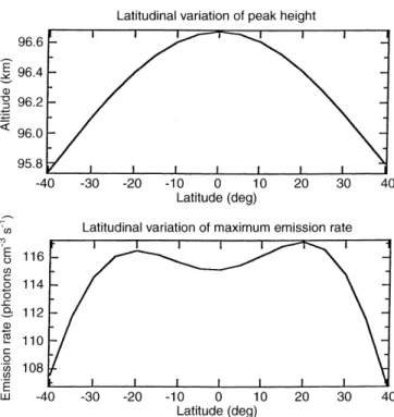
The results of the calculations for the windless atmo-sphere are displayed in Fig. 12. One can see in the top panel that the variations with latitude of the altitude of the annual mean of the emission peak are quite weak: from 96.7 km at the equator to 95.7 km at 40°latitude.
The same is true for the maximum emission rate (bottom panel). There is a minimum at the equator but, between equator and mid-latitudes, the dierence in intensities is only 8 photons cm)3s)1. These results are
Fig. 10.Latitude-height distribution of the mean green-line emission rate in October
not in agreement with the WINDII observations displayed in Fig. 9.
5 Discussion
Using radar data, Miyaharaet al.(1991) and Portnyagin
et al. (1995) obtained mean meridional and vertical winds for dierent months and for annual mean. It is important to compare our results with the results provided by these authors, because the data bases are dierent in terms of distribution and methods of measurements. Indeed, WINDII data cover January 1992±March 1994, while the radar measurements extend over 30 years. In the MLT region, an interannual variability of the wind parameters is acknowledged and we cannot exclude its in¯uence on the corresponding results. Also, the two data sets do not have the same coverage in latitude and altitude, WINDII observed up to 120 km, but is limited polarwards of 60°latitude.
Ra-dar data extend up to 90°, but are restricted to 110-km
latitude.
Furthermore, Miyaharaet al.(1991) have developed a numerical model which is not always found in agreement with their empirical results. This is why comparisons are important to derive the real atmo-sphere properties.
5.1 The annual mean meridional wind
With respect to the Portnyagin et al.(1995) results, the global structures are very close in terms of wind velocity, cell distribution and wind magnitude.
5.2 The annual mean vertical wind
The Portnyagin et al. (1995) results present a wind structure in cells which are quasi-anti-symmetrical with a latitudinal shift towards the southern hemisphere. This structure is not what we derived, but the wind ampli-tudes are in agreement (1±2 cm s)1).
5.3 Mean vertical winds in October and January
The WINDII results for October as shown in Fig. 7 indicate a symmetrical distribution in latitude. For the same month, the Miyaharaet al.(1991) empirical model also shows a latitudinal shift of the cells towards the southern hemisphere. The wind magnitudes are in agreement. These authors also present the results of their numerical model. Surprisingly, an equatorial ascendance and two tropical subsidence are predicted in very good agreement in cell positions and wind magnitudes with the WINDII results as shown in Fig. 7. We note the altitude dierence of the equatorial ascendance of about 5 km higher in the WINDII results and the agreement of the wind velocity. The WINDII results shown in Fig. 8 for the month of January are compared with the empirical model of Miyahara et al.
(1991), which exhibits an ascendance in the northern hemisphere around 87 km. Again WINDII and this model present an altitude shift. This shift is reduced when comparing with the numerical model.
5.4 Dynamical implications
Following Miyahara et al. (1991), the mean zonal acceleration and the net adiabatic and cooling rate are approximated at ®rst order byfvandN2w, respectively. In these terms, f ÿ2Xsinu, where X is the angular
velocity of the Earth andN2 the squared Brunt-VaÈisaÈlaÈ frequency. Figure 13 depicts the latitude-height distri-bution of the mean zonal Coriolis acceleration calculat-ed from our mean meridional wind ®eld for the month of January. In the winter hemisphere at mid-latitudes, we identify a region of easterly acceleration which extends from 85 to 95 km. A similar pattern is present in the summer hemisphere but westerly directed. Referring to the numerical simulations by Miyahara et al.(1991), this situation re¯ects the interaction between vertically propagating gravity waves and the mean ¯ow in the mesopause region. In this region, gravity waves may break and deposit momentum. We note the existence of signi®cant sources of momentum between 40° and 60°
latitude and above 100 km in both hemispheres. Figure 14 illustrates the mean adiabatic and cooling rate connected to the vertical motions. The latitude-height structure consists of alternating cells of heating and cooling. Same as for momentum, the signature of gravity wave breaking is present at mid-latitudes below 95 km and takes the form of a net adiabatic cooling in the northern hemisphere and heating in the southern. Referring again to the Miyahara et al. (1991)
predictions, the joint cells of heating and cooling which extend between20 latitude are related to the
dissipa-tion of the diurnal tide through eddy and molecular diusion. As in Fig. 13, there are large cells above 40°
latitude and 100 km, indicating that adiabatic heating and cooling sources are also present in this region.
Comparisons of our results with the empirical description of Miyahara et al. (1991) for January and Portnyaginet al.(1995) for the annual mean values (not presented here) show a general agreement in latitude-height structure and magnitude of cells; typically
5010ÿ5m sÿ2 for the mean zonal Coriolis
accelera-tion and 10 K per day for the adiabatic heating and cooling rate. Clearly, these three studies indicate that important sources of momentum and heating exist above 40° latitude and 100-km height which are not
predicted by numerical calculations. The possible nature of these sources has been discussed in Miyahara et al.
(1991). They suggest that gravity waves obliquely propagating from the equatorial and tropical regions can reach the lower thermosphere region and dissipate providing acceleration according to the zonal mean wind direction. They also put forward planetary waves as a possible candidate providing that the stratospheric-mesospheric regime of the mean zonal winds acts as a ducting channel to allow their propagation from one hemisphere to the other, inducing hemispheric coupling. Portnyagin et al. (1995) complement this discussion by arguing about the plausible contribution of mesoscale eddies in the MLT region.
5.5 The green-line intensity
Green-line emission has already been observed from space. Reports of such observations were, for example, presented by Donahue et al. (1973) using OGO 6 satellite or by Murphreeet al.(1984) and Elphinstoneet al.(1984) using ISIS 2 satellite. OGO 6 allowed to cover 24-h of local time in 3 months. Donahue et al. (1973) have shown that there is a depletion in the green-line emission at low latitudes which may be linked to a peculiar relationship between local time and latitude of the observations. For example, Shepherd et al. (1995) have shown that there is a large variation with local time of the green-line emission, with a marked minimum around midnight at low latitudes. This is at the opposite of mid-latitudes observations showing a maximum of emission just after local midnight (e.g. Petitdidier and Teitelbaum, 1979). The present analysis of WINDII data, as already shown, allows us to conclude that the equatorial depletion is indeed real.
Such a depletion was also deduced from the ISIS2 data analysis (Murphreeet al., 1984; Elphinstoneet al., 1984). These authors explained their observations by an enhancement of the eddy mixing at low latitudes. Vial and Teitelbaum (1986) pointed out that the ISIS2 data could also be consistent with the mean circulation induced by the dissipation of the diurnal tide in this region. Based on the mechanism proposed by Akmaev
et al. (1980), eects of tides to explain this depletion were also put forward by Forbes et al. (1993) using TIGCM simulations.
Nevertheless, from an observational point of view, WINDII allows simultaneously to measure mean wind system and green-line emission, and consequently to investigate the role of dynamics in the green-line emission process. However, WINDII observes Eulerian velocities, whereas the real mean transport is in fact due to the Lagrangian velocities which cannot be derived from the WINDII data. As already noticed, the circu-lation in the equatorial region is due to the dissipation of tides, and Vial and Teitelbaum (1986), using tidal numerical simulations, have shown that in the MLT region the Lagrangian circulation is upward and pole-ward above the equator, as the Eulerian winds described in the present study. This allows us to use WINDII data
Fig. 13. Latitude-height distribution of the mean zonal Coriolis acceleration in January
to interpret the green-line intensity distribution as a function of latitude and altitude.
We notice an ascendance at the equator, which could increase the green-line emission rate by decreasing the eect of quenching; but this is not observed. However, mean meridional wind must be also considered to play a role in the transport of constituents invoked in the emission of the green line. At the altitude of the maximum of emission, the WINDII mean meridional wind is symmetrical with respect to the equator, blowing from the equator towards mid-latitudes. Consequently, it transports oxygen away from the equator, weakening the intensity of the emission here and lowering the altitude of the emission peak as we observed. Using concentrations given by the MSIS90 model, we have calculated the vertical and meridional advection terms. It apears that they have opposite sign and that magni-tude of the horizontal advection is larger than that of the vertical one. Consequently, the meridional transport of oxygen away from equator can explain, at least partly, the equatorial depletion of green-line intensity, while the vertical transport reduces the importance of this eect.
An increase in eddy diusion could also explain the decrease in green-line intensity in the equatorial region (when compared to mid-latitudes). This explanation was, for example, put forward by Murphree et al.
(1984). Although it cannot be totally ruled out, it appears that the mean wind system, deduced from the WINDII observations, is able by itself to explain the observed dierence in the green-line intensity between equator and mid-latitudes.
6 Conclusion
1. The existence of a signi®cant annual mean circu-lation system in the MLT region is probably the most surprising result of the empirical model of Portnyagin
et al. (1995). The WINDII observations allow to maintain this conclusion. Despite some dierences in the position of wind cells, WINDII con®rms the existence of cellular structures already seen in their empirical model. Furthermore, the amplitudes of the mean annual winds deduced from WINDII are in good agreement with those of Portnyaginet al.(1995) of the order of a few metres per second for the meridional wind and a few centimetres per second for the vertical component.
2. A symmetry is found at equinoxes with an ascendance in the equatorial region. This feature was observed independently in October and April. January and July results are consistent, showing that the equatorial ascendance is shifted towards the winter hemisphere.
3. Comparisons for solstices and equinoxes with the empirical model of Miyahara et al. (1991) exhibit general agreement in the cellular structure, but also some discrepancies, probably linked to the dierence in data coverage. Furthermore, cells observed by WINDII appear to be displaced upwards with respect to the Miyahara et al. (1991) empirical and numerical model
results. However, WINDII results appear closer to the numerical simulations of Miyaharaet al.(1991) than to their empirical model, at least equatorwards of 30°
latitude.
4. In particular we con®rm here the importance of the diurnal tide dissipation in the MLT region. It is the most important factor to explain the dynamical state of the equatorial zone of the MLT region. Although this has theoretically been known a long time, both the Mi-yahara et al. (1991) and Portnyagin et al. (1995) empirical models did not reproduce clearly what was expected from numerical modelling.
5. Another important point is that WINDII data con®rm the need for additional momentum and energy sources to those presently assumed, in order to explain the actual meridional and vertical mean wind distribu-tions in the MLT region. This was a conclusion reached by Miyahara et al.(1991), comparing numerical simu-lation results to their empirical model, and by Portnya-gin et al. (1995), analysing the mean annual wind system. Even if our results exhibit some dierences in term of the position of wind cells when compared to the empirical models described by these authors, these dierences are weak enough to con®rm their conclu-sions. WINDII does not allow to sample the atmosphere polewards of 72°latitude; but it allows us to extend up
to 120 km the Portnyagin and Miyahara analysis. In particular these authors pointed out the possible impor-tance of dissipation of planetary waves in the lower thermosphere. These waves are detectable with WINDI instrument. We intend to correlate the variations in their intensities to the change in the mean wind system to con®rm (or discon®rm) this hypothesis.
6. We have investigated the role of the dynamics in the latitudinal distribution of the green-line emission rate. We have shown that predictions using MSIS90 and the mechanism proposed by Barth are not in agreement with the WINDII observations. The vertical and meri-dional advection terms have been calculated and found to be of opposite sign, meridional advection being signi®cantly larger. Thus, the green-line depletion at the equator could be generated by the meridional transport attenuated by the equatorial ascendance. We acknowl-edge that other processes have to be considered, but conclude that dynamics could be the main driving mechanism.
7. Further work on green-line modelling including photochemistry and dynamics is anticipated.
Acknowledgements. The WINDII project is sponsored by the Canadian Space Agency and the Centre National d¢Etudes Spatiales. Additional support for science analysis is provided by the Service d¢AeÂronomie of the Centre National de la Recherche Scienti®que.
The editor-in-chief thanks S. Miyahara and Yu. Portnyagin for their help in evaluating this paper.
References
applications to tidal variations of the OI(5577 AÊ) airglow, J. Atmos. Terr. Phys.,42,705±716, 1980.
Basley, B. B., and A. C. Riddle, Monthly mean values of the mesospheric wind ®eld over Poker Flat, Alaska,J.Atmos.Sci.,
41, 2368±2375, 1984.
Coy, L., D. C. Fritts, and J. Weinstock,The Stokes drift due to vertically propagating internal gravity waves in a compressible atmosphere,J.Atmos.Sci.,43,2636±2643, 1986.
Donahue, T. M., B. Guenther, and R. J. Thomas,Distribution of atomic oxygen in the upper atmosphere deduced from OGO 6 airglow observations,J.Geophys.Res.,78,6662±6689, 1973.
Ebel, A.,Heat and momentum sources of the mean circulation at an altitude of 70 to 100 km,Tellus,26,325±333, 1974.
Elphinstone, R. D., J. S., Murphree, and L. L. Cogger,Dynamics of the lower thermosphere consistent with satellite observa-tions of the 5577 A airglow, II, Atomic oxygen, local turbu-lence and global circulation results,Can.J.Phys.,62,382±395, 1984.
Forbes, J. M., R. G. Roble, and C. C. Fesen,Acceleration, heating, and compositional mixing of the thermosphere due to upward propagating tides,J.Geophys.Res.,98,311±321, 1993.
Forbes, J. M., M. K. Kilpatrick, D. Fritts, A. H. Manson, and R. A. Vincent, Zonal mean and tidal dynamics from space: an empirical examination of aliasing and sampling issues, Ann.
Geophysicae, this issue, 1997.
Gault, W. A., G. Thuillier, G. G. Shepherd, S. P. Zhang, R. H. Wiens, W. E. Ward, C. Tai, B. H. Solheim, Y. Rochon, C. McLandress, C. Lathuillere, V. Fauliot, M. HerseÂ, C. Hersom, R. Gattinger, L. Bourg, M. D. Burrage, S. J. Franke, G. Hernandez, A. Manson, R. Niciejewski, and Vincent, R. A., Validation of O(1S) wind measurements by WINDII: the WIND Imaging Interferometer on UARS,J.Geophys.Res.,101,10441±10554, 1996.
Hedin, A. E.,Extension of the MSIS thermosphere model into the middle and lower thermosphere, J. Geophys. Res., 96, 1159± 1172, 1991.
Hedin, A. E., E. L. Fleming, A. H. Manson, F. J. Schmidlin, S. K. Avery, and S. J. Franke,Empirical wind model for the middle and lower atmosphere,NASA Technical memorandum 104581 & 104592, 1993.
McDade, I. C., D. P. Murtagh, R. G. Greer, P. H. G. Dickinson, G. Witt, J. Stegman, E. J. Llewellyn, L. Thomas, and D. B. Jenkins,
ETON2: Quenching parameters for the proposed precursors of O2 b1Rgand O(
1
S) in the terrestrial nightglow,Planet.Space Sci.,34,789±800, 1986.
Meek, C. E., and A. H. Manson, Vertical motions in the upper atmosphere from the Saskatoon (52°N, 107°W) M. F. Radar,J.
Atmos.Sci.,46,850±858, 1989.
Miyahara, S., Yu. I. Portnyagin, J. M. Forbes, and T. V. Solovjeva,
Mean zonal acceleration and heating of the 70±110-km region,
J.Geophys.Res.,96,1225±1238, 1991.
Murphree, J. S., R. D. Elphinstone, and L. L. Cogger,Dynamics of the lower thermosphere consistent with satellite observations of the 5577 A airglow, I, method of analysis,Can. J.Phys.,62,
370±381, 1984.
Murtagh, D. P., G. Witt, J. Stegman, I. C. McDade, E. J. Llewellyn, F. Harris, and R. G. H. Greer, An assessment of proposed O(1S) and O2 b1Rgnightglow excitation parameters,
Planet.Space Sci.,38,43±53, 1990.
Petitdidier, M., and H. Teitelbaum, O(1S) excitation mechanism and atmospheric tides,Planet.Space Sci.,27,1409±1419, 1979.
Portnyagin, Yu. I., J. M. Forbes, T. V. Solovjeva, S. Miyahara, and C. DeLuca,Momentum and heat sources of the mesosphere and lower thermosphere regions 70±110 km,J.Atmos.Terr.Phys.,
57,967±977, 1995.
Reid, I. M.,Some aspects of Doppler radar measurements of the mean and ¯uctuating components of the wind ®eld in the upper and middle atmosphere, J. Atmos. Terr. Phys., 45, 467±484, 1987.
Shepherd, G. G., G. Thuillier, W. A. Gault, B. H. Solheim, C. Herson, J. M. Alunni, J. F. Brun, S. Brune, P. Charlot, D. L. Desaulniers, W. F. J. Evans, F. Girod, D. Harvie, R. H. Hum, D. J. W. Kendall, E. J. Llewellyn, R. P. Lowe, J. Ohrt, F. Pasternak, O. Peillet, I. Powell, Y. Rochon, W. E. Ward, R. H. Wiens, and J. Wimperis, The wind imaging interferometer on the Upper Atmosphere Research Satellite,J.Geophys.Res.,98,
10725±10750, 1993.
Shepherd, G. G., C. McLandress, B. H. Solheim,Tidal in¯uence on O(1S) airglow emission rate distributions at the geographic
equator as observed by WINDII,Geophys.Res.Lett,22,275± 278, 1995.
Thuillier, G., V. Fauliot, M. HerseÂ, and L. Bourg,MICADO wind measurements from Observatoire de Haute-Provence for the validation of WINDII green-line data, J. Geophys. Res.,101,
10431±10440, 1996.
Vial, F., and H. Teitelbaum, The role of tides in the thermody-namics of the lower thermosphere for solstice conditions, J.