References
Information about the authors
T. Zelinsky
REGIONAL POVERTY LEVELS IN THE EUROPEAN UNION:
A SPATIAL ECONOMETRIC APPROACH
1The main objective of this study is to analyze the most important determinants of monetary poverty (at the macro-level) in the European Union, taking into account the effects of regional spillovers. Regression analyses of spatial data in the period 2007–2009, i.e. the pre-crisis and crisis years are performed in order to compare the size of the impact of the selected variables on poverty levels. In the study, a spatial Durbin model (SDM) is employed and the sample includes 187 EU regions. In order to quantify the impacts of the explana
-tory variables, scalar summary measures are used (the average direct impacts, as well as the indirect and to
-tal impacts of income, are negative).
Keywords: monetary poverty, spatial Durbin model, regional spillovers, European Union
1. Introduction
With respect to the economic crisis and high unemployment levels, living conditions, poverty and inequality research attracts attention from researchers from different disciplines. The conse -quences of the economic crisis include the widen -ing of the gap between rich and poor and the wors -ening living conditions (not only) of the poorest. In this paper, we focus on the regional poverty lev -els in the European Union, where over 80 million EU citizens are estimated to be poor (based on the monetary concept). In terms of poverty research nowadays, the researchers focus on the develop -ing countries, as well as the developed countries (see e. g. [1], [2], [3], [4]).
The assessment of well-being for poverty anal -yses is usually based on two main conceptual ap -proaches: the welfarist approach and the non-wel -farist approach [5]. The wel-farist approach as -sumes that individuals are rational and able to make production and consumption choices that maximize their utility. A lack of command over commodities measured by low income or con -sumption is the working deinition of poverty in terms of the welfarist conceptual approach [6]. The non-welfarist approach recognizes two basic con -cepts: the basic needs concept linked to A. K. Sen’s [7] functioning’s concept and the capabilities con -cept, also introduced by A. K. Sen [8]. The meas -urement of well-being following the welfarist ap -proach is based on proxies, such as income, con -sumption or expenditure data, and following the non-welfarist approach it is based on proxies such as material deprivation [9].
Several analyses of poverty at the regional level in the European Union have been performed. Several papers investigate poverty and its regional aspects in the European Union (see e.g. [10], [11], [12], [13], [14], [15]). As a contribution to poverty research in the European Union at the regional level, the main objective of this study is to ana -lyse the most important determinants of mone -tary poverty (at the macro-level) in the European Union, taking into account the effects of regional spillovers. Regression analyses of spatial data in the pre-crisis year of 2007 and the crisis years of 2008/2009 are performed in order to compare the size of the impact of the selected variables. In this study, a spatial Durbin model (SDM) is employed and the sample includes 187 EU regions. In order to quantify the impacts of the explanatory varia -bles, scalar summary measures are used (the aver -age direct impacts, as well as the indirect and to -tal impacts, of income are negative). All the esti -mations, calculations and graphical outputs were performed in the R environment [16] using the li
-braries spdep [17], rgdal [18], maptools [19] and shape [20].
2. Description of the Model 2.1. The Spatial Durbin Model
In this study, a spatial Durbin model (SDM), given by Eq. (1), is employed. The rationale be -hind this model is to incorporate the spatial ef -fects working through the dependent variable and the spatial effects working through the explana -tory variables.
y=ιnα+Xβ+ρWy+WXγ + ε (1) where y — is an n-by-1 vector of observations of at-risk-of-poverty rates (natural logarithms are used); ιn — is an n-by-1 vector of ones with the as -sociated scalar parameter α;X — is an n-by-q ma -trix of observations of the four explanatory vari -ables (natural logarithms of all the vari-ables are used) with the associated vector parameter β;W — is an n-by-n non-stochastic spatial weight matrix specifying the spatial dependence among regions. In accordance with [21], W is based on the nearest neighbours with k = 6. When region j is a neigh -bour of region i, W
ij = 1, and Wij = 0 otherwise. The diagonal elements of W are set to zero by conven -tion. W is row-standardised, which ensures that all the weights are between zero and one, while the sum of the weights in each row is one (as six nearest neighbours are used, the spatial weights equal 1/6); Wy — is an n-by-1 spatial lag vector of y with an associated scalar spatial dependence parameter (the parameter of the irst-order spa -tial autoregressive process) ρ, and is assumed to lie within the interval (−1, 1). In our model, we as -sume that 0 <ρ< 1, which indicates that the re -gional at-risk-of-poverty rates are positively re -lated to the at-risk-of-poverty rates in neighbour -ing regions; WX — is an n-by-q matrix of the spa -tially lagged explanatory variables with associated vector parameter γ;ε — is an n-by-1 normally dis -tributed, constant variance disturbance term,
(
2)
0, n .
N εI
ε ∼ σ
2.2. Observation Units and Description of the Data
regions), Norway (7 NUTS-2 regions), Poland (6 NUTS-1 regions), Romania (8 NUTS-2 regions), Sweden (8 NUTS-2 regions), Slovenia (2 NUTS-2 regions), Slovakia (4 NUTS-2 regions) and the United Kingdom (12 NUTS-1 regions).
The at-risk-of-poverty rate as the dependent variable and four explanatory variables (dispos -able per capita income, long-term unemployment rate, education level and population density) are employed in the survey. In order to assess the po -tential inluence of the economic crisis on the es -timated impacts, all the variables refer to the ob -servation years 2007, 2008 and 2009 (complete data sets were not available for 2010 and 2011).
The at-risk-of-poverty rate [arop] (after so -cial transfers) is deined as the share of persons with an equivalised disposable income below the risk-of-poverty line, which is set at 60% of the na -tional median equivalised disposable income after social transfers. The disposable income is deined as the gross income less income tax, regular taxes on wealth and compulsory social insurance contri -butions, while the gross income is the total mon -etary and non-mon-etary income received by the household over a speciied income reference pe -riod. Income is measured at the household level, and in order to gain the equivalised disposable in
-come, the total disposable income of a household has to be divided by the equivalised household size according to the modiied OECD scale (giving a weight of 1.0 to the irst adult, 0.5 to other per -sons aged 14 or over and 0.3 to each child younger than 14).
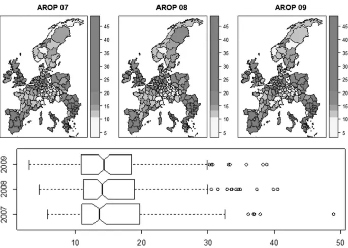
Figure 1 depicts the distribution of the at-risk-of-poverty rate across the EU regions. It is obvious that regions with a high at-risk-of-poverty rate are concentrated in the eastern and southern part of the European Union. The boxplots further indicate that the mean value of the poverty rate increased between 2007 and 2009, but the notches measur -ing the signiicance of the difference between the two medians indicate that the differences among the medians are not statistically signiicant.
The disposable per capita income [income] is the total income of a household, after tax and other deductions, that is available for spending or saving, divided by the number of household mem -bers. The disposable per capita income is meas -ured in terms of the purchasing power standard based on the inal consumption per inhabitant.
The long-term unemployment rate [unempl] is the share of people who are out of work and have been actively seeking employment for at least a year, and is measured as a percentage.
As a proxy for the education level [edu], the share of persons aged 25–64 with pre-primary, primary or lower secondary education attainment is used. The category pre-primary, primary or lower secondary education refers to the ISCED-97 levels 0–2.
The population density [density] is measured in terms of the number of inhabitants per square kilometre.
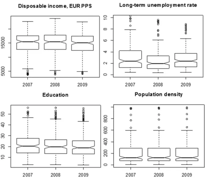
Figure 2 depicts the distribution of the ex -planatory variables between 2007 and 2009. The notched boxplots indicate that there are no statis -tical differences in the medians among the years; on the other hand, however, the long-term unem -ployment rate distribution indicates a decrease in the median long-term unemployment rate be -tween 2007 and 2008 followed by an increase be -tween 2008 and 2009.
The spatial autocorrelation of the variables was further investigated (see Table 1). All the var -iables except for population density are signii -cantly positively spatially autocorrelated, i.e. sim
-ilar values occur near one another. Moran’s I sta -tistics (for the statistically signiicant spatial au -tocorrelation) range between 0.3995 and 0.7678.
In the proposed regression model, the at-risk-of-poverty rate in region i (denoted by yi) depends on the poverty rates in the neighbouring regions (as deined in the spatial weight matrix W) cap -tured by the spatial lag variable W
iy, where Wi is the i th row of the spatial weight matrix W. It fur -ther depends on the own-region levels of dispos -able per capita income, long-term unemployment rate, education and population density (given by the i th row of matrix X) as well as the levels of dis -posable per capita income, long-term unemploy -ment rate, education and population density in the neighbouring regions, represented by W
iX. Taking into account the relationships among the neighbouring regions, a change in the q th var -iable in region i has not only a direct impact on the at-risk-of-poverty rate of this region, but also an indirect impact on other regions j≠i. The esti -mated model will be discussed in terms of direct,
indirect and total effects, as proposed by [22], and the interpretation follows [23].
3. Results
The estimation results of the spatial Durbin model and the quantiication of the explanatory variables on the at-risk-of-poverty rates are pre -sented in this section. In order to quantify the im -pacts of the explanatory variables, the scalar sum -mary measures suggested by [22] are used.
3.1. Model Estimation
In order to discriminate between the unre -stricted spatial Durbin model and the spatial er -ror model, i.e. between substantive and residual dependence, a likelihood ratio test is used. A like -lihood ratio test rejects the null hypothesis of a spatial error model speciication (test statistics: 507.1 (2007 model), 374.6 (2008 model) and 420.9 (2009 model) with the corresponding p-values: < 0.0001). This supports our belief that the spatial externalities are substantive rather than random. The estimated spatial autoregressive parameters (ˆρ2007=0.6685,ˆρ2008=0.6900 and ˆρ2009=0.4648) provide evidence of signiicant spatial effects work -ing through the dependent variable. A variance in -lation factor measure was used to check for possi -ble multicollinearity in the model.
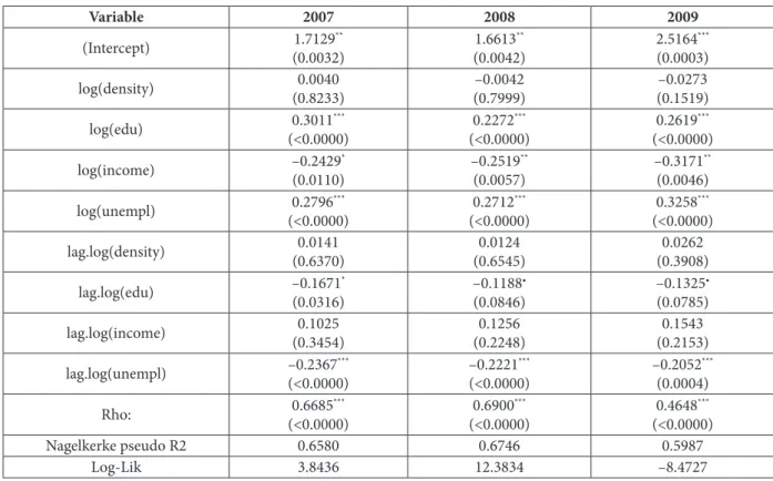
In Table 2, we can see that three non-spatially lagged explanatory variables (education, dispos -able income and long-term unemployment) and two spatially lagged explanatory variables (edu -cation and long-term unemployment) are statis -tically signiicant. Taking into account that the quantiication of the impacts of the explanatory variables is based on direct, indirect and total ef -fects, as suggested by [22], the output in Table 2 is not of great importance for interpretation pur -poses regarding the impact of the explanatory variables.
As pointed out by [23], estimates associated with spatially lagged variables are often incor -rectly interpreted as measures of the size and sig -niicance of indirect impacts in spatial regression models. In the case of our model, the indirect ef -fects of education and long-term unemployment would be interpreted incorrectly (both spatially lagged variables are statistically signiicant, but the indirect impacts are statistically insigniicant according to Table 3).
3.2. Impacts’ Estimates
This section focuses on the interpretation of the estimated model in terms of the direct, indi -rect and total effects (Table 3). The average di-rect impacts, or in other words the impact of changes in the i th observation of x
q, denoted as xiq, on yi are similar in spirit to typical regression coeficient interpretations [22]. The direct impacts include feedback inluences arising as a result of the im -pacts passing through neighbours and back to the observation itself [24].
The average indirect impacts represent the to -tal impact on the individual observation yi result -ing from chang-ing the q th explanatory variable by the same amount across all n observations. On the other hand, the average indirect effects also repre -sent impacts on an observation, i.e. how changes in all the observations inluence a single observa -tion i.
The average total impacts are represented by the sum of the average direct effects and the av -erage indirect effects. If the values of the q th ex -planatory variable change by the same unit in all the regions, the value of the dependent variable will change by
(
1)
1q
−
−ρ β units. In other words, the average total impacts relect how a one-per -cent change in the qth explanatory variable in all the regions inluences the dependent variable in a typical (average) region.
Table 1
Spatial autocorrelation of the variables (Moran’s I statistic)
Variable 2007 2008 2009
arop 0.5578
***
(<0.0001)
0.5898***
(<0.0001)
0.5128***
(<0.0001)
density 0.0368
(0.2489)
0.0367 (0.2498)
0.0368 (0.2490)
edu 0.7672
***
(<0.0001)
0.7678***
(<0.0001)
0.7630***
(<0.0001)
income 0.7579
***
(<0.0001)
0.7333***
(<0.0001)
0.7436***
(<0.0001)
unempl 0.4165
***
(<0.0001)
0.3995***
(<0.0001)
0.4433***
(<0.0001)
4. Discussion and Conclusions
As expected, the average direct impact of in -come is negative, the impact of unemployment is positive and the impact of education is positive as
well. If the median income increases in region i, the poverty rate is likely to decrease in the same region. On the other hand, a rise in the long-term unemployment rate in a region i results in an in
-Table 2
Estimated coeicients
Variable 2007 2008 2009
(Intercept) 1.7129 ** (0.0032) 1.6613** (0.0042) 2.5164*** (0.0003) log(density) 0.0040 (0.8233) –0.0042 (0.7999) –0.0273 (0.1519) log(edu) 0.3011 *** (<0.0000) 0.2272*** (<0.0000) 0.2619*** (<0.0000) log(income) –0.2429 * (0.0110) –0.2519** (0.0057) –0.3171** (0.0046) log(unempl) 0.2796 *** (<0.0000) 0.2712*** (<0.0000) 0.3258*** (<0.0000) lag.log(density) 0.0141 (0.6370) 0.0124 (0.6545) 0.0262 (0.3908) lag.log(edu) –0.1671 * (0.0316) –0.1188• (0.0846) –0.1325• (0.0785) lag.log(income) 0.1025 (0.3454) 0.1256 (0.2248) 0.1543 (0.2153) lag.log(unempl) –0.2367 *** (<0.0000) –0.2221*** (<0.0000) –0.2052*** (0.0004) Rho: 0.6685 *** (<0.0000) 0.6900*** (<0.0000) 0.4648*** (<0.0000)
Nagelkerke pseudo R2 0.6580 0.6746 0.5987
Log-Lik 3.8436 12.3834 –8.4727
Signif. codes: 0 ‘***’ 0.001 ‘**’ 0.01 ‘*’ 0.05 ‘•’ 0.1 ‘ ’ 1 Source: own construction
Table 3
Estimated impacts
Impacts log(density) log(edu) log(income) log(unempl)
Direct 2007 0.0065 (0.6861) 0.3062*** (0.0000) –0.2520** (0.0057) 0.2721*** (0.0000)
2008 –0.0027
(0.9056) 0.2333*** (0.0000) –0.2597** (0.0033) 0.2656*** (0.0000) 2009 –0.0262 (0.1614) 0.2611*** (0.0000) –0.3166** (0.0036) 0.3216*** (0.0000) Indirect 2007 0.0479 (0.5100) 0.0980 (0.4621) –0.1718 (0.3255) –0.1426 (0.1765) 2008 0.0291 (0.7397) 0.1163 (0.3548) –0.1478 (0.4698) –0.1072 (0.3289) 2009 0.0243 (0.6365) –0.0193 (0.8435) 0.0125 (0.9196) –0.0963 (0.2064) Total 2007 0.0544 (0.4775) 0.4042*** (0.0007) –0.4238* (0.0152) 0.1295 (0.2925) 2008 0.0264 (0.7712) 0.3496** (0.0027) –0.4075* (0.0360) 0.1584 (0.1542) 2009 –0.0019 (0.9695) 0.2418** (0.0013) –0.3041** (0.0092) 0.2253** (0.0023)
crease in the poverty rate in the same region, and the same is true for a rise in the share of persons aged 25–64 with pre-primary, primary or lower secondary education attainment, i.e. a rise in the share of such persons is associated with a rise in the poverty rate.
According to the results, none of the variables employed in the model has statistically signiicant indirect impacts. As already mentioned, the spa -tially lagged coeficients’ estimates indicated sta -tistically signiicant indirect effects, but in fact those are not statistically signiicant.
Summing up, the average direct effects and av -erage indirect effects yield statistically signiicant positive average total impacts of education and negative average total impacts of income. The re -sults further indicate a statistically signiicant av -erage total impact of long-term unemployment on the at-risk-of-poverty rate in 2009. This is due to the direct impact size of the rise in unemployment in 2009.
Taking into account the time period (the pre-crisis year 2007 and the crisis years 2008 and 2009), certain changes appear in the estimated impacts. The size of the direct impacts of educa -tion and unemployment decreased between 2007 and 2008 and increased between 2008 and 2009, while the increase in the size of the long-term un -employment impact is signiicantly higher than the increase in the low education impact. As for the average direct impact of income, its size (in absolute terms) increased over the whole survey period and rose by more than 20 per cent between 2007 and 2009.
On the other hand, taking into account spill -over effects, the size of the total average im -pacts (in absolute terms) decreased in the case of the low education level as well as disposable income between 2007 and 2009. The size of the long-term unemployment rate’s direct average impact rose by almost 75 per cent between 2007 and 2009, and became statistically signiicant.
This might be explained by the rise in the long-term unemployment rate and the at-risk-of-pov -erty rate between 2008 and 2009, and unemploy -ment is considered one of the most important factors of poverty. As for the spillover effects, the results propose an interesting inding. The total average impacts of the low education level, long-term unemployment and disposable income were stronger than the direct average impacts in 2007 and 2008. Then the situation changed and the to -tal average impacts became weaker than the di -rect average impacts in 2009. This might be asso -ciated with the changed overall economic condi -tions in the European Union and its regions with respect to the consequences of the economic cri -sis in Europe.
The results indicate that the space matters in explaining poverty. Analysing poverty (similarly to other economic phenomena) without taking space into account results in a loss of important information concerning space.
Like every piece of research, the present study has its shortcomings. The relativity of poverty concept is one of its important limitations. Cross-national or cross-regional comparisons based on relative poverty measures are quite compli -cated and do not necessarily relect the differ -ences among countries or regions. The availabil -ity of data at the regional level is the most impor -tant limitation of poverty analyses. Many of the EU countries do not publish poverty data at the regional level (and many of them do not publish the variable “region” in the micro-data set), which makes poverty analyses at the regional level very dificult. On the other hand, we have to be aware of the shortcomings of regional data based on a limited number of observations resulting in bi -ased estimates. Taking into account the hetero -geneity across the EU regions, the availability of suitable data on poverty at the regional level is crucial for performing quality analyses as well as for policy implications.
Acknowledgement and Disclaimer
his work was supported by the Slovak Scientiic Grant Agency as part of the research projects VEGA 1/0127/11 Spatial Distribution of Poverty in the European Union and VEGA 2/0004/12 Paradigms of the Future Changes in the 21st Century (Geopolitical, Economic and Cultural Aspects). he EU-SILC data sets were made available for the research on the basis of contract No. EU-SILC/2011/33, signed between the European Commission, Eurostat and the Technical University of Kosice. Eurostat has no responsibility for the results and conclusions, which are those of the researcher.
References
1. Ravallion M. (2009). he Crisis and the World’s Poorest. Development Outreach, 11, 3, 16-18.
2. Pressman S., Scott R. (2009). Consumer debt and the measurement of poverty and inequality in the USA. Review of Social Economy, Vol. 67, 2,127-148.
3. Copeland P., Daly M. (2012). Varieties of poverty reduction: Inserting the poverty and social exclusion target into Europe 2020. Journal of European Social Policy, Vol. 22, 3, 273-287.
5. Ravallion M. (1992). Poverty Comparisons: A Guide to Concepts and Methods. Washington DC: he World Bank. ISSN 0253-4517.
6. Duclos J. Y., Araar A. (2006). Poverty and Equity: Measurement, Policy and Estimation with DAD. New York: Springer. ISBN 978-0387-33318-2.
7. Sen A. K. (1984). he Living Standard. Oxford Economic Papers, New Series. Vol 36, Supplement: Economic heory and Hicksian hemes, 74-90.
8. Sen A. K. (1999). Commodities and Capabilities. New Delhi: Oxford University Press, 1999. ISBN 0-19-565038-7.
9. Zelinsky T. (2010). Analysis of Poverty in Slovakia based on the Concept of Relative Deprivation. Politicka ekonomie. Vol. 58, 4, 542-565.
10. Forster M., Jesuit D., Smeeding T. (2003). Regional Poverty and Income Inequality in Central and Eastern Europe. WIDER Discussion Papers. World Institute for Development Economics (UNU-WIDER), No. 2003/65.
11. Betti G. et al. (2005). Comparative Indicators of Regional Poverty and Deprivation: Poland versus EU-15 Member States. Comparative Economic Analysis of Households’ Behaviour (CEAHB): Old and New EU Members. Warsaw 30 September — 1 October, 2005.
12. Verma V., Betti G., Natilli M., Lemmi A. (2006). Indicators of Social Exclusion and Poverty in Europe’s Regions. Working Paper n. 59. Siena: Department of Quantitative Methods, University of Siena.
13. Quintano C., Castellano R., Punzo G. (2007). Estimating Poverty in the Italian Provinces using Small Area Estimation Models. Metodoloski zvezki, Vol. 4, 1, 37-70.
14. Pirani E., Schiini D’Andrea, S. Vermunt J.K. (2009). Poverty and social exclusion in Europe: diferences and similarities across regions. 26 IUSSP Conference, Marrakech.
15. Betti G. et al. (2012). Subnational indicators of poverty and deprivation in Europe: Methodology and applications. Cambridge Journal of Regions, Economy and Society. Vol. 5, 1, 129-147.
16. R Core Team (2012). R: A language and environment for statistical computing. R Foundation for Statistical Computing, Vienna, Austria. ISBN 3-900051-07-0.
17. Bivand R. et al. (2013). spdep: Spatial dependence: weighting schemes, statistics and models. R package version 0.5-56. 18. Keitt T. H. et al. (2013). rgdal: Bindings for the Geospatial Data Abstraction Library. R package version 0.8-4. 19. Lewin-Koh N. U. (2013). maptools: Tools for reading and handling spatial objects. R package version 0.8-22. 20. Soetaert K. (2012). shape: Functions for plotting graphical shapes, colors. R package version 1.4.0.
21. LeSage J., Fischer M. M. (2008). Spatial Growth Regressions: Model Speciication, Estimation and Interpretation. Spatial Economic Analysis. Vol. 3, 3 (2008), 275-304.
22. LeSage J., Pace R. K. (2009). Introduction to Spatial Econometrics. New York: CRC Press, 2009. ISBN 978-1-4200-6424-7.
23. Fischer M. M. et al. (2010). he impact of human capital on regional labour productivity in Europe. In Fischer, M. M., Getis A. (eds): Hadbook of Applied Spatial Analysis. Springer, Berlin, Heidelberg and New York, pp. 583-597.
24. Fischer M. M., Wang J. (2011). Spatial Data Analysis: Models, Methods and Techniques. Berlin: Springer, 2011. ISBN 978-3-642-21719-7.
Information about the author
Zelinsky Tomas (Kosice, Slovakia) — PhD, Associate Professor, Department of Regional Science and Management, Faculty of Economics, Technical University of Kosice (32, Nemcovej, Kosice, 04001 Slovakia, e-mail: [email protected]).
I. V. Danilova, A. V. Rezepin