The distribution of average and marginal effective tax rates in European Union member states

The Distribution of Average and Marginal Effective Tax Rates in

European Union Member States.

Herwig Immervoll

University of Cambridge;

European Centre for Social Welfare Policy and Research, Vienna

Abstract

Macro-based summary indicators of effective tax burdens do not capture differences in effective tax rates facing different sub-groups of the population. They also cannot provide information on the level or distribution of the marginal effective tax rates thought to influence household behaviour. I use EUROMOD, an EU-wide tax-benefit microsimulation model, to compute distributions of average and marginal effective tax rates across the household population in fourteen European Union Member States. Using different definitions of ‘net taxes’, the tax base and the unit of analysis I present a range of measures showing the contribution of the tax-benefit system to household incomes, the average effective tax rates applicable to income from labour and marginal effective tax rates faced by working men and women. In a second step, effective tax rates are broken down to separately show the influence of each type of tax-benefit instrument. The results show that measures of effective tax rates vary considerably depending on incomes, labour market situations and family circumstances. Using single averages or macro-based indicators will therefore provide an inappropriate picture of tax burdens faced by large parts of the population.

Keywords: Effective Tax Rates; European Union; Microsimulation.

JEL Classification: H22; D31; C81

Address for correspondence: Department of Applied Economics University of Cambridge

The Distribution of Average and Marginal Effective Tax Rates in the

European Union.

Herwig Immervoll1

Draft Version (09-08-02).

Please do not quote without author’s permission.

1. Introduction

The analysis of most tax and transfer policy issues requires knowledge about how much is paid in taxes and received in benefits, by whom and in what circumstances. Moreover, in assessing existing tax-benefit policies and proposing reforms, it is useful to compare levels and structures of taxes and benefits across countries. The complexity of relevant rules governing tax liability and benefit entitlement and a lack of comprehensive and comparable data at the micro-level has led to major efforts being directed towards finding methods to construct simple summary indicators such as implicit effective tax rates based on revenue statistics and national accounts data (Carey and Tchilinguirian, 2000; Martinez-Mongay, 2000). While these measures can provide important insights regarding aggregate payments they cannot answer questions about their detailed incidence.2 Since they are normally derived

1

Research Associate at the Microsimulation Unit in the Department of Applied Economics, University of Cambridge and Research Fellow at the European Centre for Social Welfare Policy and Research, Vienna. Address for correspondence: Microsimulation Unit, Department of Applied Economics, University of Cambridge, Sidgwick Avenue, Cambridge, CB3 9DE, UK. Email: h.immervoll@econ.cam.ac.uk. This paper was written as part of the MICRESA project, financed by the Improving Human Potential programme of the European Commission (SERD-2001-00099). I acknowledge the contributions of all past and current members of the EUROMOD consortium to the construction of the EUROMOD model. The views expressed in this paper as well as any errors are my own responsibility. In particular, this applies to the interpretation of model results and any errors in its use. EUROMOD is continually being improved and updated. The results presented here represent work in progress.

EUROMOD relies on micro-data from 11 different sources for fifteen countries. These are the European Community Household Panel (ECHP) made available by Eurostat; the Austrian version of the ECHP made available by the Interdisciplinary Centre for Comparative Research in the Social Sciences; the Living in Ireland Survey made available by the Economic and Social Research Institute; the Panel Survey on Belgian Households (PSBH) made available by the University of Liège and the University of Antwerp; the Income Distribution Survey made available by Statistics Finland; the Enquête sur les Budgets Familiaux (EBF) made available by INSEE; the public use version of the German Socio Economic Panel Study (GSOEP) made available by the German Institute for Economic Research (DIW), Berlin; the Survey of Household Income and Wealth (SHIW95) made available by the Bank of Italy; the Socio-Economic Panel for Luxembourg (PSELL-2) made available by CEPS/INSTEAD; the Socio-Economic Panel Survey (SEP) made available by Statistics Netherlands through the mediation of the Netherlands Organisation for Scientific Research - Scientific Statistical Agency; and the Family Expenditure Survey (FES), made available by the UK Office for National Statistics (ONS) through the Data Archive. Material from the FES is Crown Copyright and is used by permission. Neither the ONS nor the Data Archive bear any responsibility for the analysis or interpretation of the data reported here. An equivalent disclaimer applies for all other data sources and their respective providers cited in this acknowledgement. All errors and views expressed are the responsibilities of the authors.

2

by looking at monetary aggregates without considering the institutional rules as they apply to each taxpayer and benefit recipient, they also cannot capture the extents to which taxes and benefits affect incentives of people in different circumstances. This paper aims to fill these gaps by providing detailed measures of both average and marginal effective tax rates facing households in Europe. It uses an EU-wide microsimulation model (EUROMOD) to produce distributions of these measures across households in fourteen Member States of the European Union (EU).

Effective tax rates capture the net tax burden resulting from the interaction of different types of taxes and contributions on one hand and benefit payments on the other. Average effective tax rates (AETRs) express the resulting net payments as a fraction of the income on which they are levied. They are therefore useful in assessing the size of transfers given the incomes and circumstances observed at a given point in time. Marginal effective tax rates (METRs), on the other hand, measure the degree to which any additional income would be ‘taxed away’. METRs are therefore useful measures for evaluating the financial incentives to engage in activities meant to generate or increase income.

The accurate measurement of AETRs and METRs is important for a range of policy related questions which continue to receive attention in both academic and policy circles. Measures of effective tax rates have, for instance, been used as explanatory variables in studies concerning the influence of tax burdens on economic growth (Agell, et al., 1997; , 1999), unemployment (Daveri and Tabellini, 2000; Martinez-Mongay and Fernández-Bayón, 2001) and wage setting behaviour (Sorensen, 1997). Clearly, many of the processes underlying these issues are strictly linked to the behaviour of individuals or households. In comparing and evaluating different tax-benefit systems one would therefore want to characterise them not only in terms of the effective tax burden of a single ‘representative’ agent3 but also in terms of the number and types of households and individuals who are, in fact, facing effective tax rates of the various magnitudes. In fact, from a distributional point of view, detailed knowledge about the incidence of tax and benefit payments is of interest in itself (e.g., Mercader-Prats, 1997).

Although comparable and detailed household micro-data have become more readily available in recent years, the information contained in these data sources is nevertheless insufficient for calculating detailed AETRs and METRs. One reason is simply that variables on income tax (IT) or social insurance contributions (SIC) are often missing. Even if they are recorded, social insurance contributions paid by employers (or benefit paying institutions) on behalf of employees will usually not be available (as shown below, employers’ contributions represent an important part of the tax burden borne by labour incomes). To overcome this problem simulation methods are frequently used to impute such missing information (Immervoll and O'Donoghue, 2001a; Weinberg, 1999). This basically entails combining the information on people’s status and incomes with a detailed representation of tax-benefit rules and provides all necessary information for computing AETRs.

The incorporation of detailed tax-benefit rules in microsimulation models has two other distinct advantages. They allow analysts to evaluate the effects on tax and benefit amounts of

3

changes of either the tax-benefit rules or the characteristics of households. The latter is necessary in order to compute METRs. By varying each observation’s incomes by a certain amount and then re-computing tax liabilities and benefit entitlements, the effective tax burden on any additional income can be captured. Secondly, effective tax rates can be computed under a range of different policy configurations. In the EU, such ‘forward-looking’ analyses of the likely impact of policy reforms on effective tax burdens are particularly relevant given the identification of ‘high’ or ‘excessive’ levels of taxation as a major policy concern.4

The plan for this paper is as follows. Section 2 provides a rationale for evaluating effective tax rates at the micro-level and compares approaches using empirical micro-data to macro-based techniques as well as methods macro-based on ‘synthetic’ households. Section 3 discusses the choices to be made in measuring effective tax rates and explains the precise approach adopted in the present study. The following sections present simulation results for fourteen countries. While section 4 provides household-level AETRs across all households taking into account all relevant taxes and benefits, section 5 focuses on the effective taxation of labour incomes. It presents individual-level estimates of the total tax ‘wedge’ resulting from the combination of IT and SIC. Section 6 evaluates relevant financial incentives for the working population by computing METRs. All results are presented in terms of their overall distribution of effective tax rates across the relevant populations as well as grouping by age, gender and other household characteristics. In discussing policy reforms targeted towards altering effective tax rates it is essential to understand which particular tax-benefit instruments are responsible for observed tax burdens. The distributions of METRs and AETRs are therefore decomposed in order to show the contributions of individual tax-benefit instruments. Section 7 concludes.

2. Measuring effective tax rates – why look at the micro-level?

International comparisons of tax systems have long relied on information about formal tax rules (such as the rate structure) or they have summarised their aggregate impact by relating total receipts to national income (these indicators are sometimes called ‘tax ratios’). One main shortcoming of this latter approach is that it disregards the tax base a tax is levied on. A ‘tax ratio’ for a certain type of income tax of x% may be the result of a combination of (a) a broad tax base and a low tax rate; or (b) a narrow tax base and a high tax rate. The economic consequences are, obviously, very different. To rectify this problem, there has, starting in the 1990s, been a growing interest in methods seeking to derive measures of effective tax rates based on Revenue Statistics and National Accounts (Lucas Jr, 1990, Mendoza, et al., 1994). By relating tax receipts to the relevant tax bases they provide a much better indicator of tax burdens. They are also attractive in that deriving comparable figures across countries is facilitated by the availability of internationally comparable sources of revenue statistics, such as those produced by the OECD, and standardised national accounts data.

Obviously, macro-based measures cannot be used to investigate the micro-level incidence of tax payments. There are, however, other potential problems. One is related to the institutional characteristics in terms of how taxes and benefits are integrated in different countries and the fact that macro-based effective tax rates tend to focus on taxes and SIC while disregarding

4

benefits. Child related payments may, for instance, be formally administered through the tax system in some countries (e.g., by means of refundable tax credits) and be paid as benefits in others. Clearly, excluding benefit payments in such cases means that the comparability of effective tax rates across countries will suffer. While, in principle, applying appropriate corrections would be straightforward, data on social transfers tends to be less comparable across countries than revenue statistics and incorporating them in multi-country studies can therefore be problematic.

Technical difficulties also arise due to conceptual differences between revenue statistics and national accounts data. The former are, for instance, collected on a cash basis while the latter measure incomes as they accrue. As a result the timing of the two data sources diverges (Jacobs and Spengel, 1999). Several other issues are also related to differences in definitions and scope between the two data sources and a number of assumptions are required to align them (Carey and Tchilinguirian, 2000). This range of potential problems has prompted a number of ‘health warnings’ being issued in order to make users of macro-based effective tax rates aware of their shortcomings (OECD, 2000b; c). The Working Party No. 2 on Tax Policy Analysis and Tax Statistics of the OECD Committee on Fiscal Affairs takes the view that “AETR results relying on aggregate tax and national accounts data are potentially highly misleading indicators of relative tax burdens and tax trends” and that “further work relying on micro-data is required to assess the magnitude of potential biases to average tax rate figures derived from aggregate data.”5

In fact, there is an existing literature documenting various approaches of combining information on statutory tax rules and tax returns with data on income distribution and household surveys (Barro and Sahasakul, 1986; Easterly and Rebelo, 1993). Among researchers interested in the macroeconomic effects of taxation, however, these attempts have been met with some scepticism (although some authors have in fact used them as yardsticks for validating macro-based results) as it is considered doubtful whether “marginal tax rates that apply to particular individuals in a household survey, or a specific aggregation of incomes based on tax-bracket weights, are equivalent to the aggregate tax rates that affect macroeconomic variables as measured in national accounts.”6 This limitation certainly holds for tax rate calculations based on ‘typical’ households (such as OECD, 2000a) as such estimates, while illustrative, fail to take into account the heterogeneity of the population. Although extending these calculations to a wider range of ‘synthetic’ households can serve to improve our understanding of the mechanics built into tax-benefit systems the point remains that any calculations based on synthetic households cannot capture, in the correct proportions, the tax and benefit payments across the entire range of household types found in the population as a whole (Immervoll, et al., 2001). In contrast, calculations based on representative household micro-data can be used to derive aggregate measures of effective tax rates using any desired aggregation rule. At the same time, they are more informative than aggregate measures since they capture the distribution of effective tax rates across the population.

5

Carey and Tchilinguirian (2000), p. 5. 6

As they are calculated based on statutory tax and benefit rules they are also particularly useful where a detailed knowledge of the structure and mechanics built into tax-benefit systems is important. There are two main cases where computing measures based on observed past tax receipts and tax bases (sometimes referred to as ‘backward-looking’ in the literature) cannot be used. First, measuring METRs requires assessing what would happen to tax burdens if incomes were to change. As tax-benefit systems are generally far from proportional, aggregate income changes are meaningless in this context. Instead, it is important whose income is changing. In a non-proportional tax-benefit system, METRs can therefore only be computed based on a knowledge of the distributions of incomes and other characteristics that determine tax liabilities and benefit entitlements. This problem is usually acknowledged in studies using macro-based measures of effective tax rates. However, since many of the distortionary effects of taxation that researchers are interested in are related to marginal rather than average tax rates, there is a worrying tendency to equate METRs with AETRs and use the latter as proxies for the former (see Mendoza, et al., 1994 for an example and Padovano and Galli, 2001 for a critique).

A second area where ‘forward-looking’ methods of computing effective tax rates are particularly useful is in the analysis of policy reforms. There is often a need to evaluate reforms before detailed macro-economic data become available. Since the delays can be sizable simulation techniques can play an important role in an early evaluation of policy reforms.7 By changing the parameters of the tax-benefit rules built into such simulation models, they can also be used to perform analyses of hypothetical or prospective reforms.

3. Whose taxes, which incomes, what margins?

Several choices have to be made when measuring effective tax rates. Most of them have important implications for the interpretation of the results and thus require some consideration. In fact, depending on the research questions it will often be desirable to compute effective tax rates in several different ways. A method which allows some flexibility is therefore valuable.

Before discussing the various decisions to be made and how microsimulation methods can be used to accommodate them it is useful to clarify the scope of the measurement exercise. AETRs measure some concept of total tax as a fraction of some concept of tax base. Obviously, the incidence of AETRs is therefore connected with the incidence of taxes. In studying questions of incidence one can be interested in the payments per se, or in the economic loss suffered by the taxpayer. For a particular taxpayer, this loss will, for two reasons, generally differ from the tax paid. First, taxes may, through influences on supply and demand at the market level, influence the prices of the goods and service produced or consumed by the taxpayer. Second, the taxpayer herself may, in response to price changes, adjust the basket of goods and service she produces or consumes and suffer welfare losses in the process. The familiar process of tax ‘shifting’ is of great interest to economists and any results on final incidence may be very sensitive to the degree of shifting.8

7

Martinez-Mongay (2000) notes that there is generally a 2-3 year lag in the production of macro-based tax rates. 8

Moreover, there are many economic consequences of taxation that cannot be captured by looking at the amounts of taxes alone. To take an extreme example, a tax that, at a given point in time, generates no revenue at all may be detrimental to economic growth if it has made a certain type of productive activity so financially unattractive as to drive people away from engaging in it altogether. Nevertheless, it is difficult to deny that tax payments are an issue of public interest in themselves and therefore deserve investigation. The central issue then is to “distinguish clearly between tax payments and losses from taxation, and to recognise that the first is an accounting characteristic of a particular equilibrium, while the second requires the evaluation of a comparison between two alternative equilibria.”9

In this paper, effective tax rates are computed for a given ‘equilibrium’ as characterised by the information recorded in household micro-data of a particular year. While the resulting AETRs will, for the reasons stated above, not capture total losses associated with the imposition of taxes, any substitution effects caused by them do enter the results: If we assume that we are, in fact, looking at an equilibrium then people will already have adjusted their activities in response to the tax burdens imposed on them.10 The aim of computing AETRs is to understand the extent and incidence of burdens resulting from tax payments and, to avoid confusion, there should be no claim that the incidence of AETRs can be used as some sort of approximation of the incidence of economic losses (relative to the tax base). Instead, tax payments are one component of incidence analyses and should be treated as such.11 For METRs, on the other hand, no qualifications regarding any decisions about the appropriate treatment of tax shifting are required at all. The main reason why we are interested in METRs in the first place is their possible effect on behaviour or, in other words, their role in moving from ‘equilibrium 1’ to ‘equilibrium 2’. Clearly, METRs must therefore be evaluated under ‘equilibrium 1’.

While some of the methodological issues to be considered for effective tax rate measurement at the micro-level are similar or can at least be related to those facing researchers concerned with deriving macro-based measures, others only become apparent due to the level of detail which micro-based approaches support. Even though these issues exist, in principle, regardless of the level of aggregation, the data sources used for macro-based measures simply do not provide the same range choices. The relevant dimensions are (1) the types of taxes and benefits to take into account and the income (or ‘tax base’) to relate them to and (2) the unit of analysis and, related to it, the sharing of any incomes within the unit. In the case of METRs an additional issues is (3) the nature and size of the margin to be used for computing marginal effects. Each of these will be discussed in turn.

9

Dilnot, et al. (1990), p. 213. 10

It should be emphasised that this implies an important qualification of studies looking at effects of policy

reforms on the incidence of effective tax rates. If taxes and benefits are computed for a given (pre-reform)

population then, conceptually, the assumption of an equilibrium will not be appropriate. To what extent taking into account behavioural responses following the reform would, in fact, noticeably change results is another matter. The usefulness of incorporating behavioural response in microsimulation-based policy evaluations will depend on the precise type and intent of the reform and on the extent to which underlying micro-data permit changes to be detected in a statistically meaningful way. For a discussion of some of these and related issues see Pudney and Sutherland (1994) and Creedy and Duncan (2002).

11

3.1 Tax-benefit instruments and definition of income base

Although effective tax rates are supposed to provide broad measures of net tax payments, the choice of instruments to be incorporated in such a measure is not self-evident. Most studies consider taxes and ‘tax-like’ payments. However, it is not at all clear that SIC are, for example, equivalent to income taxes and it is undoubtedly the case that the degree of equivalence differs widely across countries. While, in principle, SIC are payments made in return for insurance coverage the link between income taxes and public services is not as direct. However, cross subsidies between the various ‘pots’ of public finances often make such a distinction less meaningful. In addition, social insurance schemes are, for the most part, compulsory and not characterised by a strict actuarial link between the value of insurance services and SIC paid. The discrepancy can be seen as performing functions (such as redistribution or raising revenues) normally associated with income tax.

Section 2 has already hinted at comparability problems that can arise due to international differences in the structure of tax-benefit systems when the benefit side is ignored. As the distinction between tax concessions and benefits is more or less arbitrary, tax-benefit models which allow an integrated view on the tax-benefit system as a whole are useful in this respect. There are, however, limitations nonetheless as these models usually focus on cash instruments. As a result, there are inherent difficulties in comparing effective tax rates of countries where, say, child care payments or housing benefits are paid an cash and those where these benefits are provided ‘in-kind’ through access to subsidised child-care or housing. A related question is that about the appropriate time-horizon of the calculations. Should some measure of future benefits financed by current SIC be taken into account?

Many of these issues become somewhat clearer once one considers the appropriate definition of income which is to enter the denominator of the AETR calculations. If the purpose of studying the incidence of AETRs is assessing the distribution of the relative contribution of tax-benefit systems to current cash incomes (as in section 4) then any in-kind transfers as well as future incomes such as pension rights will be disregarded.12 Similarly, if the focus is on evaluating the total tax burden on labour (as in section 5) then any taxes or benefits which are not strictly related to labour income (such as taxes on investment income, family benefits13) should be disregarded.

3.2 Unit of analysis and sharing within units

A natural question to ask is whose effective tax rates we are interested in. Depending on the purpose, we may want to look at tax/benefit payments at the individual level, the level of the formal tax unit or some other notion of family or household. For distributional studies concerned with household welfare the household level will be appropriate (Canberra Group, 2001). In measuring the tax wedge on labour, however, one would want to relate the relevant

12

There would still be an issue of what ‘current’ means. Normally, income distribution studies take the year as their reference period (Canberra Group (2001)). In the context of effective tax rate calculations based on micro-data, this means that annual income data would be ideal. Some data sources, however, measure income over a shorter period (see appendix 1). Although these data can, of course, be annualised, time-period differences in the original data need to be borne in mind in comparative studies as income changes during the year will, for a particular household, imply that annual income is not equal to one particular month’s income times 12.

13

taxes directly to the labour incomes of those supplying labour (and hence chose the individual as the unit of analysis).

Given that one distinguishing feature of households is the sharing of common resources (and given that we do not observe the precise sharing arrangements within household) studying units of analysis smaller than the household can be problematic. A particular issue arises due to the assessment unit used in statutory tax and benefit rules. These can be quite different for different instruments in a given country (e.g., individual SIC but joint IT) and, obviously, for equivalent instruments across countries. Although recent decades have, at least in the EU, seen a trend towards individual taxation, joint tax filing is current practice in a considerable number of countries (O'Donoghue and Sutherland, 1999). In addition, even if the tax schedule itself is applied to each individual separately, tax concessions such as tax free allowances or tax credits are often transferable between family members and therefore represent a ‘joint’ element. Notions of family or household are even more important in determining the eligibility for benefits and applicable amounts. With the exception of insurance based benefits practically no type of benefit is targeted directly towards individual persons. Instead, the structure of families or households as well as their members’ characteristics and incomes are crucial determinants of benefit payments. Even insurance based benefits formally paid to the insured person often take into account family circumstances (e.g., minimum or basic pensions, unemployment benefits).

Whenever taxes or benefits are explicitly or implicitly targeted towards more than one person, the question how these payments are shared between members of an assessment unit is crucial if the unit of analysis is smaller than the unit of assessment. Should benefits be shared equally among all members of the household, or just among adults, or should payments be assigned according to some equivalence scale? Similarly, what is the best basis for sharing jointly paid income taxes? Should it be in proportion to the tax base or should those with higher income pay progressively more? Inevitably, these decisions are, to some degree, arbitrary. The value of calculations based on micro-data lies in raising the issue in the first place and forcing analysts to be explicit about the decisions they adopt.

3.3 Nature and size of margin used for computing METRs

Additional issues arise in computing the effective tax burden on marginal income changes. They relate to the exact features of the change. While marginal tax rates could in principle be found analytically by taking first differences of the relevant effective tax schedule this is not possible in practice as tax-benefit systems are characterised by discontinuities. The straightforward approach then is to derive METRs numerically simply by altering income, using a tax-benefit model to re-compute relevant taxes and benefits and comparing the results with the original situation:

METR = 1- ( ((y1 + d) (1 – t2) – y1 (1 – t1)) / d ) (1)

where y1 is the original pre-tax-benefit income, d is the margin and t1 and t2 are the AETRs

applying, respectively, to y1 and y1+d. y1(1–t1) and (y1+d)(1–t2) are, therefore, the incomes

into account in computing t1 and t2, as well as the unit of analysis used for measuring

incomes. In addition, the size (and direction) of d is important and leads to different interpretations of resulting METRs. In establishing work incentives, one will often be interested in a small income change, such as a small fixed percentage rise in earnings or the rise in gross earnings due to an additional hour of work. However, the margin can also be earnings as a whole. 1-METR is then equivalent to the concept of a replacement rate (of moving from in-work to out-of work in the case of d = -earnings and out-of-work to in-work in the case of d = potential earnings). For such ‘large’ margins, however, it is often not sufficient to only change income before re-computing taxes and benefits. In addition, several other characteristics which are available in the micro-data and which, in addition to income, are potential determinants of taxes and benefits (variables such as hours of work, employment status, economic sector) will have to be altered as well (see Immervoll and O'Donoghue, 2001c).

If one is concerned with financial incentives then the appropriate choice of a unit is particularly important. If a persons’s additional earnings reduce the household’s entitlement to housing benefits then this is likely to be a consideration she will take into account. Similarly, an important consequence of joint taxation of married couples is that, from the couple’s point of view, the lower earning spouse faces, for a lower level of earnings, the same marginal tax rate as his/her higher earning partner. Clearly, to bring out these facts, METRs would need to be computed for the relevant unit as a whole. For multi-person units, however, another decision to be made is who to attribute d to. Since for the unit as a whole, METRs will be different depending on who earns the additional amount, it will often be appropriate to evaluate different scenarios. For example, in order to separately analyse financial work incentives for men and women one may analyse METRs evaluated for the household as a whole under the alternative assumptions that female / male members of household increase their earnings (see section 5).

4. The contribution of tax-benefit systems to households’ current disposable incomes

Average effective tax rates can provide a convenient description of the degree to which household incomes are affected by taxes and benefits. The household perspective allows one to put aside issues related to the unit of analysis as discussed in section 3.2. The concern with current incomes also makes redundant any questions about the degree to which current taxes or SICs can be seen as savings financing future benefits. But an important consideration that remains is which components of current income should be counted in the numerator and denominator of the AETR. For most components such as earnings, taxes, SIC, family benefits, etc., the decision is straightforward. It is less clear-cut, however, for incomes which are partly insurance based but are also characterised by some elements of outright transfers to the recipient household. In cross-country studies, the issue is complicated by the fact that, for similar policy instruments, the “mix” between insurance and transfers varies widely across countries. This is particularly the case for pensions and unemployment benefits.

for recipients of these incomes therefore do not reflect the generosity of these instruments but the extent to which they are subject to (net) tax payments. Other replacement incomes which enter the tax base include maternity benefits, sickness benefits, disability insurance and survivor/orphan benefits. SIC paid by the employer are not part of pre-tax-benefit income. The denominator of the AETR consists of all taxes paid by the household plus compulsory own SIC minus family benefits, care benefits, social assistance/minimum income benefits and all other ‘non-replacement’ cash transfers such as housing benefits.

For each household, the relevant income components are either taken directly from the micro-data (earnings, pensions, etc.) or simulated using EUROMOD, an EU-wide tax-benefit model. The sources of micro-data used in this exercise are listed in appendix 1. The same micro-data are also used by EUROMOD as the basis for simulating income taxes, SIC as well as means-tested and universal benefit payments. A simulation of these income components is necessary in cases where they are not recorded in the micro-data. In addition, simulation is required in order to compute changes in taxes and transfers following marginal income changes (section 6). EUROMOD is an integrated microsimulation model of the tax-benefit systems of all fifteen EU Member States. It permits common definitions of income concepts, units of analysis, sharing ‘rules’, etc. to be used across countries and therefore is a suitable instrument for computing effective tax rates in a comparable or, at least, reconcilable way.14 The tax and benefit rules underlying all calculations in this paper are those for 1998.

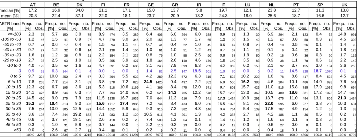
Table 1 shows the distribution of household AETRs for fourteen countries along with the number of observations for each AETR band (modal values are shown in bold typeface). Large difference between median and mean in some countries are a first indication of the spread of AETRs across the population. While the amount of taxes and own SIC paid in the country as a whole is, relative to pre-tax-benefit income, similar in Ireland and the UK, the median is very different: half of Irish households pay less than 6% in net taxes with just under 20% having their incomes entirely unaffected by the tax-benefit system. The mean average effective tax burden on pre-tax-benefit income including replacement incomes is highest in Denmark and, at about a third of the Danish level, lowest in the UK, Ireland and Spain.

Taking a closer look at the distribution we see that a considerable number of households are net benefit recipients with between 8% in Denmark and 30% in the UK having negative AETRs. For this group, non-replacement incomes exceed pre-tax benefit incomes. The fact that Denmark and the UK are the two extremes in this respect is instructive as one would a priori expect Denmark to have a more generous social transfer system. In interpreting these results it important to keep in mind that AETRs depend on both net-taxes and pre-tax-benefit incomes. If in a given country, there are more households where all household members are benefit recipients, we will therefore see a larger number of negative AETRs even if the benefits are less generous. Equally important, counting replacement incomes as pre-tax-benefit incomes will tend to push AETRs upwards for those countries with generous unemployment benefits and/or pensions: If people are entitled to these payments they will obviously be less likely to fall back on ‘last-resort’ benefits such as social assistance or other means tested transfers.

14

Given the dissimilar distributions it is interesting to analyse which household characteristics are related to the level of AETRs. The interaction of the various characteristics of interest could be captured using regression techniques. I defer this approach to future work and instead show as a first step tables focussing on one characteristic at a time. Table 2 shows how the distributions differ for different income groups.15 While in the UK the tax burden borne by the top quintile is one of the lowest, this country also has the most ‘progressive’ system in that the average AETR in the top quintile is more than 100 percentage points higher than that for the bottom 20%. This does, of course, not mean that the mechanisms built into the tax-benefit system are in themselves necessarily more ‘progressive’ than in other countries. An important factor behind these numbers is the distribution of pre-tax-benefit incomes: More unequal distributions will, for a given structure of tax-benefit system, also result in larger disparities between effective tax burdens. In particular, if low-income groups draw a very large part of their income from social transfers (UK, Finland, Greece) then AETRs can be highly negative, leading to large percentage point differences when compared to AETRs of higher income groups.16

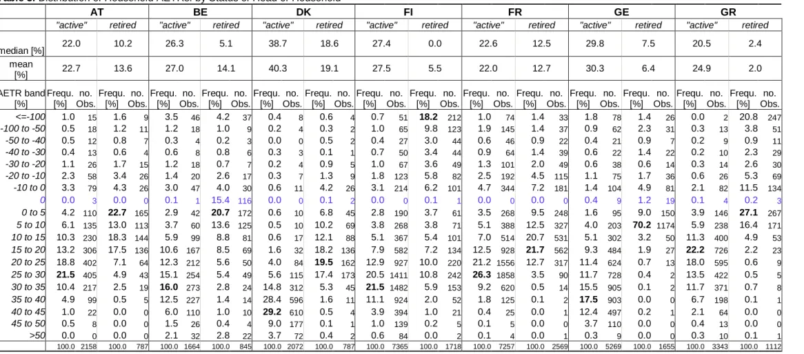
One main factor determining pre-tax-benefit incomes is the labour market status of household members. Table 3 considers two of the relevant groups; those economically “active” (employed or self-employed) and the retired. Since AETRs are computed here on a household basis the status refers to that of the head of household.17 For the groups as a whole, net taxes relative to pre-tax-benefit incomes are at least twice as high for the ‘active’ group in nine out of fourteen countries. In Ireland and Portugal the majority of households headed by a retired person do in fact face zero AETRs and are, thus, outside the scope of the tax-benefit system. While this is not the case in the UK, the mean AETR for retired people is negative indicating a large number of retired people with low pensions who are dependent on minimum income and other means-tested benefits. A large number of negative AETRs is also found among the retired group in Finland. Turning to the ‘active’ group the largest incidence of high AETRs is found in Denmark, Germany, the Netherlands and Belgium where, respectively, more than 89%, 49%, 41% and 40% of ‘active’ households are faced with AETRs in excess of 30%. The relevant proportion in the UK (2.5%) is the lowest of all fourteen countries followed by Spain with just under 4%.

Table 4 shows separate distributions for different age groups (referring, again, to the head of household) and confirms the picture of clearly lower AETRs applying to those drawing their main income from old-age pensions. One can again see a large number of zero AETRs among the ‘>65’ households in Ireland and Portugal and also Spain. Along the age profile, AETRs in all countries follow an inverted ‘U’ shape which is particularly pronounced in Finland, Germany, Greece and the UK. The largest number of net benefit recipients among households headed by young (<25) people can be found in the Netherlands followed by the UK, Finland

15

In computing quintile points, differences in household size and composition have been corrected for using the ‘modified OECD’ equivalence scale. In dividing the population into five equally sized groups, households have been weighted by their size.

16

It is instructive that, in the UK, the difference in means between the top quintile group and the first quantile with non-negative mean AETRs (quintile group 3) is one of the lowest among the fourteen countries.

17

and Germany. A final breakdown of household AETRs is provided in table 5 where distributions are presented for a range of family structures. Single parent households are subject to lower effective tax rates than the overall population in all countries. With negative medians, they are mainly net benefit recipients in seven out of fourteen countries (Belgium, France, Germany, Ireland, Luxembourg, the Netherlands and, most clearly, the UK). Again, this may be due to generous benefits being available to them (such as in Belgium18) or to a lack of earning opportunities forcing them to rely on social transfers (whatever their level) or a combination of the two. Upon first inspection it may be surprising that households without children face lower AETRs than those with children in some countries (Greece, Italy, Portugal and Spain, in particular). This is to a large extent due to retired people being part of the ‘no children’ group. Once they are excluded (column ‘No Children; Head not retired’) households with children face lower AETRs than those without in all countries but Spain where a small difference in favour of childless households remains.

How important are individual tax-benefit instruments in determining effective tax burdens? To answer this question, the various levels of AETRs in all countries have been decomposed in terms of the instruments that drive them. The results are shown in figure 1 where the contribution of each instrument to the total net taxes is shown for the different AETR bands.19 The bars all have the same total height (100%) so that a similar sized ‘tax’ section in AETR bands ’40 to 45’ and ’20 to 25’ would, for instance, indicate an average amount of income tax in the former band being about twice as large as that in the latter band. Negative components (benefits) are those which reduce net taxes in each AETR band. Note that bars have been omitted for AETR bands with fewer than 10 observations. Except for that, however, the graphs say nothing about the incidence of the various AETR levels so that it is important to read them in conjunction with table 1. In addition to the contribution of individual tax-benefit instruments figure 1 graphs, for each AETR band, average per-capita ‘tax-bases’ (i.e., pre-tax-benefit income including replacement incomes) relative the population median.20

As expected, higher tax-bases are generally subject to higher AETRs. As in table 2, however, the degree of progressivity varies across countries. Notably, we see that in four of the countries (Belgium, Greece, Italy, Spain, UK) the highest AETRs are not paid by those with the highest ‘tax-base’. This is frequently due to upper contribution limits above which no (additional) SIC are due. However, taxes other than income tax (wealth and property tax) also play a role as these may lead to high total tax burdens relative to income. The balance between taxes and SIC as revenue generating instruments differs widely. In Denmark, Finland and the UK taxes represent, throughout the AETR spectrum, more than 75% of total household payments to the government. At the other extreme, own SIC paid by Austrians markedly exceed taxes in most AETR bands. On the benefit side, we see family benefits being a particularly important contributor to net benefit receipts of low-income households in Luxembourg, Spain, Italy and Belgium. The dependence of low-income households on minimum income benefits is strongest in Greece and Ireland while housing related cash benefits play an important role in this respect in the UK, France and Germany. In Denmark

18

See Immervoll, et al. (2001). 19

‘Other Benefits’ are care benefits, educational grants and other transfers that do not fit into any of the other three benefit categories. As before, replacement incomes such as pensions or unemployment benefits are not counted as ‘benefits’ here but included in the ‘tax base’.

20

and the Netherlands, housing benefits are, as a fraction of total net taxes, largest for households with pre-tax-benefit incomes above about 40% of the median while for lower-income groups they are less important.

5. The effective tax burden on labour income

The focus in this section is on the tax burden borne by labour incomes. As briefly discussed above this means that AETRs need to be evaluated for the individuals supplying the worked hours. It also requires a different definition of ‘net taxes’ and ‘tax base’ than the exercise in section 4. First, although we are, again, only concerned with payments rather than the total ‘losses’ they give rise to, it should not matter who pays the taxes formally.21 As a result, employer SIC paid on behalf of the employee are included in the numerator of the AETR ratio along with own SIC and income taxes. Since it is the burden on total labour income we are interested in employer SIC also need to be added to employment income to yield the ‘tax base’ denominator.22 As a rule, benefits are not subtracted from the numerator. An exception are in-work benefits in the UK (Family Credit in 1998; now Working Families’ Tax Credit) which constitute a tax concession particularly designed to increase net labour incomes.23

An interesting conceptual question concerns the treatment of consumption taxes. Traditionally, it has been argued that, as they also reduce earners’ consumption opportunities, they need to be included in calculations of the ‘labour tax wedge’ by adding them to the AETR numerator.24 However, a contrasting view is that, since consumption taxes apply to both earners and non-earners, they do not constitute a ‘labour tax wedge’ and therefore do not matter for studying the relationship of tax burdens and unemployment (Daveri and Tabellini, 2000). In the results presented here, I implicitly adopt the second view as, for technical reasons, it is difficult to include consumption taxes in the fourteen country simulation exercise.25

Since AETRs are computed at an individual level rather than for the household as a whole it is necessary to assume sharing arrangements for joint income taxes. In this exercise, it is assumed that any joint income tax burdens of a joint tax unit are shared in proportion to

21

There is, however, a long-running debate whether SIC paid by employers have a stronger or more immediate effect on labour demand than own SIC. For arguments in support of this link see, for instance, Liebfritz, et al. (1997). For recent empirical evidence pointing towards little effect of payroll taxes on labour demand see Bauer and Riphahn (2002).

22

It should be noted that the calculations do not take into account components of ‘non-wage labur costs’ that cannot be simulated using household micro-data. These include payroll taxes that depend on firm-specific characteristics. However, employer SIC as simulated by EUROMOD do represent the major part of total payroll taxes. Another area where household micro-data typically do not provide detailed information is the provision of voluntary employer insurance contributions to occupational pension plans, etc. To the extent that these vary between countries, any results based on such data-sources may not adequately capture these differences. This will also be true for the numbers presented in this paper.

23

For a discussion of the properties of UK in-work benefits see, for instance, Blundell and Hoynes (forthcoming).

24

According to Layard, et al. (1991), p. 209, for instance, this wedge is “the gap between real labour costs of the firm […] and the real, post-tax consumption wage of the worker”.

25

taxable income.26 Another issue concerns the treatment of self-employment incomes which, by their nature, are part labour income and part income from capital. Carey and Tchilinguirian, 2000 present an approach which attempts to identify these components in the correct proportions at the macro-level. Due to the generally poor quality of self-employment income variables as available in micro-data sources the present paper does not attempt to approximate appropriate shares of labour and capital components and instead restricts its scope to employees only. This is important when interpreting results for countries where self-employment incomes are important (e.g., Greece, Portugal) and may frequently represent a ‘second-choice’ substitute for regular employment.

Because income taxes are levied on the sum of all taxable income it is not entirely straightforward to find the tax paid on labour income alone in cases where individuals have income from more than one source. The approach taken here is to find the average income tax rate which applies to taxable income as a whole and to assume that this rate applies uniformly to all taxable income components (a result of this assumption is that AETRs on labour incomes will tend to be underestimated in countries where other income sources, such as income from capital, are effectively taxed at a lower rate). A similar method is used for computing the average labour ‘tax’ rate due to SIC. As people can, at a given point in time, have more than one income subject to SIC (e.g., employment and self-employment income) it is assumed that the resulting average ‘tax’ rate applies uniformly to all components of the SIC base. In a last step, the average income tax and SIC rates are added up to find total AETRs on labour income.

The results for the employed population (non-civil servants and aged 18-64) are presented in table 6a.27,28 First, it is instructive to compare the mean effective tax burdens to those resulting from existing macro-based studies. There are, of course, important conceptual differences and one would therefore not expect to find similar numbers. Nevertheless, results from different studies should at least to some degree be reconcilable if they are to be useful for policy analysis purposes. In table 6b EUROMOD results for employees are compared with those reported in Martinez-Mongay, 2000: 27. In both cases, countries are ranked in descending order of AETRs. We see that EUROMOD results are higher in all fourteen countries and this is particularly true for countries such as Portugal, Greece, Italy or Spain, where tax evasion plays a role (as discussed in section 4, the results in this paper refer to theoretical tax and SIC liabilities in a situation of no tax evasion). More importantly,

26

After any deductions, i.e., the income to which the tax schedule applies. In some countries, such as Belgium, tax schedules are formally individual based but as considerable amounts of taxable income are transferable from the higher-earning to the lower-earning spouse, a sizable ‘joint’ elements exists nevertheless. In these cases, I treat the transfer as a tax-concession for higher-earning spouses, i.e., they are still assumed to pay the tax due on any transferred taxable income, albeit at the lower rate at which the lower-earnings spouse would be taxed. 27

Civil servants are excluded because the details and degree to which their insurance benefits are financed by employers vary widely across countries. Any results including civil servants would therefore be difficult to interpret. While authorities employing civil servants explicitly pay employer SIC in some countries, they can neither be identified nor simulated in others.

28

however, one should keep in mind that the micro-based approach used here is able to focus exclusively at the income taxes and SIC paid by those working during the entire year (see footnote 28) and thus isolate the effective tax burden on labour incomes alone. Macro-based AETRs are distorted in this respect as they cannot easily separate those parts of taxes and SIC levied on labour incomes from those levied on unemployment benefits, pensions, etc. There are other data-related issues that can help explain discrepancies between and micro-based AETR estimates such as a known under-representation of very high incomes in underlying household surveys (Sutherland, 2001a). With the notable exception of Luxembourg and Portugal (whose positions are swapped) as well as Italy the ordering of countries in table 6b is, nevertheless, remarkably similar for both sets of measures.

While this is somewhat reassuring the main point of computing AETRs based on micro-data is to gain an understanding of the distributions of tax burdens. We see from table 6 that they are generally less dispersed than for the household based AETRs in section 4. In particular, since the total tax burden here is defined as income tax plus SIC without any consideration for benefits, there are very few negative net tax burdens on labour incomes (tax credits can nevertheless cause negative AETRs as in Austria and the UK). Nevertheless, the width of the distribution is still considerable. AETR bands encompassing more than 10% of the working population are spread over a range of at least 15 percentage points and up to 40 percentage points in Greece. We also see a considerable number of earners where gross labour costs equal net earnings (zero AETRs in Greece, Ireland, Germany and the UK). In all fourteen countries, using aggregate or mean AETRs alone would clearly provide a poor representation of the tax burden faced by a major part of the working population.

The number of negative and zero AETRs in Germany, Greece, Ireland and the UK is sufficiently large to produce a zero median AETR for the lowest gross earnings decile group (table 7).29 Indeed, UK mean AETRs for this group are negative, indicating substantial refundable tax credits for employees with very low earnings. The highest AETRs apply to top earning levels in Belgium with income taxes, employee SIC and employer SIC summing up to more than 60% of gross earnings. The lowest effective tax burdens on very high earnings are found in Ireland and the UK. However, top earners are not always subject to the highest AETRs. In both Germany and the Netherlands, certain compulsory SIC are no longer due at all above the upper contribution limit as employees are supposed to find their own insurance. While in the Netherlands, very substantial jumps in marginal income tax rates in the high income range (from 6.35% to 50% and 60%) produce income tax burdens which more than compensate for the drop in SIC, this is not the case in Germany.

The regressive nature of SIC is even more visible in France where, in conjunction with progressive but small income taxes, they produce a very flat effective tax rate structure. This is confirmed in figure 2 showing the contribution of income tax and SIC to the various levels of effective tax burdens. Similar to figure 1 the tax base (right hand scale, here earnings plus employer SIC) is shown in relation to the median and as before, a negative bar indicates that, for this AETR band, the relevant income component reduces the AETR on average. SIC are a more important determinant of AETR than income taxes in all countries but Denmark, Ireland

29

and also the UK. With the exception of Germany, Luxembourg, the Netherlands and the UK, employer SIC represent a larger component of AETRs than own SIC (particularly in Belgium and Italy).

6. No pain no gain? Marginal effective tax rates for working men and women

Tax-benefit models can be used to numerically compute METRs by altering income variables observed in the micro-data, re-computing taxes and benefits and comparing them with taxes and benefits before the income change. As the concern here is with measuring METRs for the working population the income being changed is earnings and the chosen margin is +3%. For the purpose of this paper METRs are, for reasons stated in section 2, measured at the household level. The change in net taxes following the 3% earnings increase takes into account any changes in cash income (inclusing income taxes, own SIC and all simulated benefits).

While changes in net taxes are summed across all members of household they will generally be different depending on which members of household face the change in earnings. This is particularly important when evaluating financial incentives of higher/lower earning spouses to increase earnings. To capture these differences, METRs are computed separately for men and women. In other words, for households with female and male earners METRs are computed twice with the 3% earnings increase going, in turn, to women and men.30 The target group is restricted to the working population aged 18-64.31

Results for this group as a whole are shown in table 8. With median METRs ranging between about 25% (Portugal and Spain) and more than 50% (Denmark, Germany) women tend to face lower METRs than men in all countries but Germany. By far the largest number of earners facing METRs in excess of 50% is found in Denmark (86% of all earners) followed by Germany (60%). On the other end of the spectrum, roughly one fourth of earners in Greece and Spain (24%) would retain the full amount of a 3% earnings increase (METR equal to, or less than, zero).32 Denmark and the UK have the most concentrated distributions of METRs with 51% and 48% of the entire working population located in just one single 5 percentage point METR band (50 to 55% in Denmark; 30 to 35% in the UK).

For the latter two countries, METRs differ, in fact, very little between different (household-) income groups (table 9a). METRs between the highest and lowest decile group differ by little more than ten percentage points. In the UK, earners in the bottom two decile groups are

30

In cases where there are more than one working-age earners of the same sex each of them receives a 3% increase. The resulting METR for this household can be interpreted as an average between each of those earners. 31

However, since METRs are meaningful regardless of the type and duration of work activities the group is much less restricted and includes civil servants, the self-employed, and those with more than one labour market status during the observation period.

32

subject to considerably larger marginal tax burdens than their high-income counterparts – a result of high withdrawal rates for both means tested benefits (Income Support, Job Seekers’ Allowance, Housing Benefit, Council Tax Benefit) and in-work benefits (Family Credit) and SIC thresholds below which no contributions are payable. Among earners in the bottom decile group, women in the UK are subject to higher METRs than men and therefore appear to be more likely to face situations where large amounts of any additional earnings are effectively taxed away through benefit withdrawals. A similar spike in METRs at low income levels exists in Ireland (for women) and Portugal (for men) while in the other countries the joint effects of benefit withdrawals and tax/SIC thresholds appear to affect the working population to a lesser extent. In Denmark, the small differences in METRs between high and low income earners is less related to exceptionally high marginal rates at the bottom than to a very flat income tax schedule.

This is also visible in table 9b showing METRs by individual earnings deciles. The most interesting dimension here, however, is that of gender differentials. While METRs for the working population as a whole were generally lower for women we now see a more diverse picture. In countries with joint income tax filing, women tend to face higher METRs than men in the same earnings group (France, Germany, Ireland, Luxembourg, Portugal, Spain). For some decile groups, noticeable differences also exist where there are tax systems that, although not formally employing a joint tax base, allow sizable parts of income or tax concessions to be transferred from the higher- to the lower earnings spouse. The scatter plot in figure 3 illustrates the direction and extent of METR gender differentials across countries: Those cases in table 9b where METRs for women exceed those for men in the same earnings group are below the 45-degree line (and vice versa). Overall, this points towards higher METRs for women overall although the situation differs widely between countries.

Taking a closer look at which tax-benefit instruments drive METRs the important role of benefits is clearly visible in figure 4. The withdrawal of means-tested benefits is the major contributor to very high (>80%) METRs in all countries but Greece, where the withdrawal of income tax concessions is more important.33 These are also very relevant in the UK where the tapering-away of in-work benefits has a noticeable effect. We also note that, throughout all countries, the highest METRs are not faced by the highest-earning individuals but by those earnings (often substantially) less than the median earner (dashed line in figure 4). Indeed, those living on incomes below the poverty threshold are clearly more likely to face situations where very high parts of any additional earnings are lost mainly through lower benefits (table 10). Such ‘poverty traps’ can be identified in all countries, again with the exception of Greece where means-tested benefits are generally less important.

33

7. Conclusion

The aim of this paper was to introduce a micro-simulation based methodology to assess effective tax rates and to present results for fourteen EU Member States. It was argued that effective tax burdens faced by people can differ substantially depending on the particular labour market and household situation and that these differences matter when assessing the economic consequences of tax-benefit systems.

The distributions of both average and marginal effective tax rates show that summing up the effective tax burden using one single average or macro-based figure can provide very misleading pictures of effective tax burdens for large numbers of people. Micro-based measures of effective tax rates therefore have an important role in enriching and complementing indicators based on macro-data or ‘typical household’ type calculations. In addition, marginal effective tax rates are impossible to derive looking at aggregates alone. The results in this paper show that differences between average and marginal effective tax rates in both level and distribution can be substantial and that using average tax rates as proxies for marginal rates will therefore often be problematic.

One attraction of computing macro-based effective tax rates is that it is relatively straightforward and, given the availability of consistent data across countries, can easily be implemented across different countries. An assessment of effective tax burdens at the micro-level, on the other hand, is confronted with a large number of conceptual and definitional issues as the discussion in this paper has shown. This is particularly true when comparing rates across a number of countries. This multitude of measurement issues raises two relevant questions. First, is it feasible? Given the effort needed to build simulation models, harmonise micro-data and keep both policy rules and data sources undertaking comprehensive multi-country studies on a regular basis seems difficult. Microsimulation models, however, are useful for a multitude of purposes (e.g., Atkinson, 2002). Similar to micro-data they can therefore be considered as research infrastructure. If supported as such the effort and amount of resources needed for any particular study will become less prohibitive as synergies between different model applications are exploited.

Tables and Graphs.

Table 1. Distribution of Household Average Effective Tax Rates

AT BE DK FI FR GE GR IR IT LU NL PT SP UK

median [%] 17.2 16.9 34.0 21.1 17.1 15.0 13.7 5.8 19.7 12.1 23.8 12.7 11.3 13.8

mean [%] 20.3 22.4 37.1 22.0 18.1 23.7 20.9 13.2 24.3 18.0 25.6 18.7 16.6 12.7

AETR band [%]

Frequ. [%]

no. Obs.

Frequ. [%]

no. Obs.

Frequ. [%]

no. Obs.

Frequ. [%]

no. Obs.

Frequ. [%]

no. Obs.

Frequ. [%]

no. Obs.

Frequ. [%]

no. Obs.

Frequ. [%]

no. Obs.

Frequ. [%]

no. Obs.

Frequ. [%]

no. Obs.

Frequ. [%]

no. Obs.

Frequ. [%]

no. Obs.

Frequ. [%]

no. Obs.

Frequ. [%]

no. Obs. <=-100 2.3 75 5.7 150 3.0 75 8.9 474 3.5 389 6.4 406 6.0 294 6.0 158 0.9 71 1.3 30 6.9 294 2.1 123 0.4 32 14.8 991

-100 to -50 1.2 46 1.5 41 0.9 27 4.7 279 3.0 345 2.0 156 1.3 77 1.7 65 1.3 90 1.5 42 1.2 57 0.8 50 0.3 14 4.5 302

-50 to -40 0.7 24 0.6 17 0.4 10 1.5 94 1.1 115 0.7 41 0.4 22 1.0 45 0.6 47 0.8 23 0.4 19 0.5 26 0.1 3 1.4 95

-40 to -30 0.7 27 1.2 32 0.6 14 2.1 138 1.4 156 1.0 61 1.0 51 1.2 43 0.7 57 1.1 28 0.1 9 0.4 22 0.1 7 1.8 125

-30 to -20 1.6 58 1.2 36 0.8 21 2.2 154 2.1 237 0.8 79 1.0 55 2.5 90 0.8 68 1.9 50 0.2 15 0.6 36 0.3 20 1.7 116

-20 to -10 2.7 98 2.5 63 1.0 32 3.5 255 3.9 427 1.8 164 2.6 140 4.6 179 1.8 140 3.5 83 0.9 38 1.1 78 0.6 34 2.2 149

-10 to 0 4.0 129 3.5 92 1.6 44 4.7 391 6.2 685 3.1 243 7.9 399 6.3 259 4.2 359 6.2 159 2.1 92 3.7 155 3.0 194 3.6 250

0 0.9 28 6.3 144 0.1 4 0.0 1 0.0 1 1.4 82 2.5 147 19.5 601 1.0 70 0.0 0 0.2 11 14.5 828 18.7 1070 0.1 9

0 to 5 9.7 324 10.0 250 2.4 67 3.3 294 5.5 622 4.2 289 12.3 572 6.3 315 7.1 522 10.2 222 1.8 78 8.6 417 8.4 522 4.5 313

5 to 10 7.8 268 7.7 214 3.1 89 3.8 378 7.2 823 24.5 1425 9.4 497 7.2 382 6.8 556 16.2 383 4.6 204 10.1 486 14.0 893 7.6 541

10 to 15 12.3 406 6.7 195 3.6 115 5.3 518 10.6 1169 4.1 369 8.4 475 12.0 571 9.7 803 15.7 423 11.0 515 15.8 785 17.9 1089 9.8 694

15 to 20 14.1 476 8.9 244 6.3 192 7.7 794 14.0 1594 6.2 529 14.3 765 12.2 578 15.7 1293 13.0 362 10.5 480 18.6 881 17.2 1078 14.7 1048

20 to 25 14.5 490 9.0 275 7.9 265 11.5 1238 16.7 1935 7.0 644 11.3 616 7.9 341 17.3 1424 10.9 291 13.7 675 11.0 494 13.1 805 21.3 1434

25 to 30 15.3 455 10.4 313 9.0 326 15.6 1717 17.4 1985 7.2 744 8.4 433 6.0 230 16.5 1375 8.1 202 22.0 995 6.0 227 3.8 230 10.3 631

30 to 35 7.5 244 10.0 305 12.5 421 14.4 1652 5.9 643 9.3 915 7.3 382 4.3 146 9.4 764 5.4 139 17.5 787 4.9 154 1.2 65 1.3 83

35 to 40 3.6 108 7.4 244 19.2 632 7.1 983 1.2 129 10.5 911 4.1 201 1.3 42 4.2 335 2.7 65 4.2 186 1.1 36 0.5 32 0.2 14

40 to 45 0.6 23 3.7 121 19.1 619 2.6 418 0.2 26 7.4 500 1.3 64 0.1 3 1.4 112 1.2 30 1.6 68 0.1 3 0.3 20 0.0 0

45 to 50 0.3 8 1.0 31 5.8 180 0.7 144 0.0 5 2.2 110 0.2 13 0.0 0 0.2 19 0.3 7 0.6 27 0.0 0 0.1 6 0.0 0

>50 0.0 0 2.6 67 2.7 82 0.4 88 0.1 5 0.2 9 0.2 11 0.0 0 0.4 30 0.0 0 0.4 18 0.1 5 0.1 5 0.0 2

100.0 3287 100.0 2834 100.0 3215 100.0 10010 100.0 11291 100.0 7677 100.0 5214 100.0 4048 100.0 8135 100.0 2539 100.0 4568 100.0 4806 100.0 6119 100.0 6797

Source: EUROMOD, author’s calculations.