Use of Artificial Neural Network for Testing Effectiveness of Intelligent Computing Models for Predicting Shelf Life of Processed Cheese

Journal of

Computer Science and Control Systems

Vol.

5

, Nr.

2

,

October

201

2

University of Oradea Publisher

University of Oradea, Faculty of Electrical Engineering and Information Technology

S

EDITOR IN-CHIEF

Eugen GERGELY - University of Oradea, Romania

EXECUTIVE EDITORS

Gianina GABOR - University of Oradea, Romania Daniela E. POPESCU - University of Oradea, Romania Helga SILAGHI - University of Oradea, Romania Viorica SPOIALĂ - University of Oradea, Romania

ASSOCIATE EDITORS

Mihail ABRUDEAN Technical University of Cluj-Napoca, Romania Lorena ANGHEL I.N.P. Grenoble, France

Gheorghe Daniel ANDREESCU "Politehnica" University of Timisoara, Romania Angelica BACIVAROV University Politehnica of Bucharest, Romania Valentina BALAS “Aurel Vlaicu” University of Arad, Romania Barnabas BEDE The University of Texas at El Paso, USA Dumitru Dan BURDESCU University of Craiova, Romania

Petru CASCAVAL "Gheorghe Asachi" Technical University of Iasi, Romania Horia CIOCARLIE "Politehnica" University of Timisoara, Romania

Tom COFFEY University of Limerick, Ireland

Geert DECONINCK Katholieke Universiteit Leuven, Belgium Ioan DESPI University of New England, Armidale, Australia Jozsef DOMBI University of Szeged, Hungary

Toma Leonida DRAGOMIR "Politehnica" University of Timisoara, Romania Ioan DZITAC Agora University of Oradea, Romania János FODOR Szent Istvan University, Budapest, Hungary Voicu GROZA University of Ottawa, Canada

Kaoru HIROTA Tokyo Institute of Technology, Yokohama, Japan Stefan HOLBAN "Politehnica" University of Timisoara, Romania Štefan HUDÁK Technical University of Kosice, Slovakia Geza HUSI University of Debrecen, Hungary Ferenc KALMAR University of Debrecen, Hungary Jan KOLLAR Technical University of Kosice, Slovakia Tatjana LOMAN Technical University of Riga, Latvia Marin LUNGU University of Craiova, Romania Anatolij MAHNITKO Technical University of Riga, Latvia Ioan Z. MIHU “Lucian Blaga” University of Sibiu, Romania Shimon Y. NOF Purdue University, USA

George PAPAKONSTANTINOU National Technical University of Athens, Greece Dana PETCU Western University of Timisoara, Romania Mircea PETRESCU University Politehnica of Bucharest, Romania Emil PETRIU University of Ottawa, Canada

Mircea POPA "Politehnica" University of Timisoara, Romania Constantin POPESCU University of Oradea, Romania

Dumitru POPESCU University Politehnica of Bucharest, Romania Alin Dan POTORAC "Stefan cel Mare" University of Suceava, Romania Dorina PURCARU University of Craiova, Romania

Nicolae ROBU "Politehnica" University of Timisoara, Romania Hubert ROTH Universität Siegen, Germany

Eugene ROVENTA Glendon College, York University, Canada Ioan ROXIN Universite de Franche-Comte, France

Imre J. RUDAS Tech Polytechnical Institution, Budapest, Hungary

Rudolf SEISING European Centre for Soft Computing, Mieres (Asturias), Spain Ioan SILEA "Politehnica" University of Timisoara, Romania

Lacramioara STOICU-TIVADAR "Politehnica" University of Timisoara, Romania Athanasios D. STYLIADIS Alexander Institute of Technology, Greece Lorand SZABO Technical University of Cluj Napoca, Romania Janos SZTRIK University of Debrecen, Hungary

Honoriu VĂLEAN Technical University of Cluj-Napoca, Romania Lucian VINTAN "Lucian Blaga" University of Sibiu, Romania Mircea VLADUTIU "Politehnica" University of Timisoara, Romania Şahin YILDIRIM Erciyes University, Turkey

ISSN 1844 - 6043

CONTENTS

DACHIN Tudor1_{, MEZA Serban}2_{, NEMES Marian}3 _{,VODA Adriana}4_{, BADILA Florin}5 _- 1_{University “Lucian Blaga”} of Sibiu, Romania, 2_{Technical University of Cluj-Napoca, Romania,} 3_{Continental Automotive Systems S.R.L.,} Sibiu, Romania, 4_{iQuest Technologies, Cluj-Napoca, Romania,} 5_{Wenglor Electronic, Sibiu, Romania}

Complexity Appreciation for BLDC Flat Top Sinus Implementation...5

GOYAL Sumit, GOYAL Kumar Gyanendra - National Dairy Research Institute, Karnal, India

Use of Artificial Neural Network for Testing Effectiveness of Intelligent Computing Models for Predicting Shelf

Life of Processed Cheese...9

HANGIU Radu-Petru, FILIP Andrei-Toader, MAR IȘ Claudia Stelu a, BIRÓ Károly Ágoston - Technical University of Cluj-Napoca, Romania

A Z-Source Inverter for an Integrated Starter Alternator...15

HARLIŞCA Ciprian, SZABÓ Loránd - Technical University of Cluj-Napoca, Romania

Real-Time Simulation Environment for Embryonic Networks ...19

MARGINEAN Calin1_{, MARGINEAN Ana-Maria}1_{, VESE Ioana}1_{, TRIFA Viorel}1_{, TRIFU Emil}2 _- 1_Technical University of Cluj-Napoca, Romania, 2_{S.C. TRAMBUS S.R.L., Cluj-Napoca, Romania}

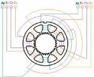
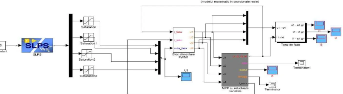
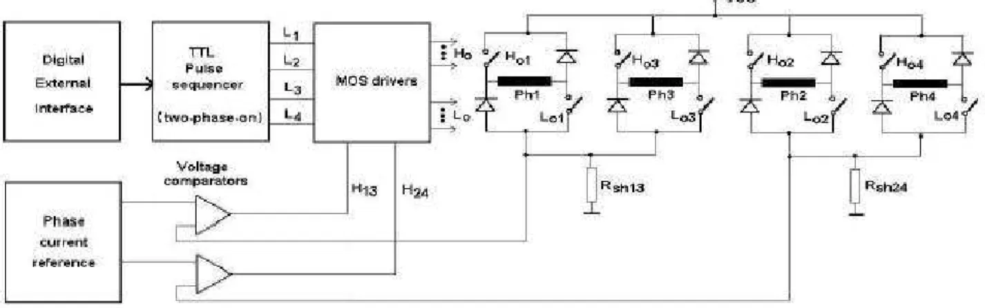
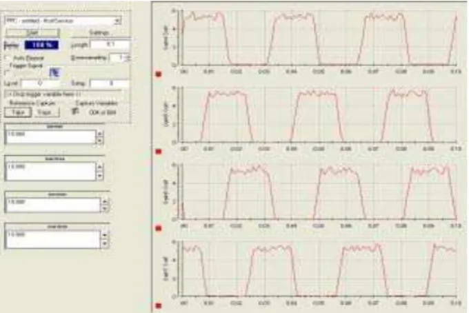
Design and Implementation of a PWM Inverter for Reluctance Motors...23

RAMAKRISHNAN Sumathi1_{, MAHALINGAM Usha}2 _- 1_{Pavai College of Technology, Namakkal, India,} 2_Sona College of Technology, Salem, India

Microstructure Development by Controlling Grain Size ...27

STOJANOVIC Igor, ZDRAVEV Zoran, TASEVSKI Angel - ‘Goce Delcev’ University, Stip, Macedonia

Progressive Wavelet Correlation as a Tool for Recognition of the Images...33

VIATTCHENIN Dmitri - National Academy of Sciences of Belarus, Minsk, Republic of Belarus

Complexity Appreciation for BLDC Flat Top Sinus Implementation

DACHIN Tudor

, MEZA Serban

, NEMES Marian

,VODA Adriana

, BADILA Florin

1 _{Universitatea “Lucian Blaga” Sibiu, Bd. Victoriei Nr.10, Sibiu, [email protected]}

2 _{Universitatea Tehnica Cluj-Napoca, Str. Constantin Daicoviciu Nr. 15, Cluj-Napoca, [email protected]} 3 _{Continental Automotive Systems S.R.L., Str. Salzburg Nr.8, Sibiu, [email protected]}

4 _{iQuest Technologies, Str. Motilor Nr.6-8, Cluj-Napoca, [email protected]} 5 _{Wenglor Electronic, Str. Caprioarelor nr. 2, Sibiu, [email protected]}

Abstract - The paper presents the usage of a better

commutation technique taking into account existing simulation and calculation models. An implementation is suggested, after performing an accurate study of the motor and the control system. The need for predefining the needed space and calculus capability is a must in complex projects, therefore the proposal is to pre-calculate most of the required inputs and use look up tables inside the software processing.

Keywords: flat top sinus commutation, simulations, mathematical model, driving technique.

I. INTRODUCTION

Automotive applications that make use of Brushless Direct Current (BLDC) motors have gained popularity due to energy efficiency advantages, energy/volume ratio and increased diversity and availability of application specific control chips. BLDC motors, in comparison with DC motors, have a longer service life, do not have high emissions (caused by brush sparking), can be used in harsher environments (e.g. hydraulic or transmission gear oil), require smaller available volume and can be driven with very high powers. A BLDC motor has the similar efficiency as permanent magnet synchronous machines. Especially due to energy consumption concerns and the need to improve overall system efficiency, usage of BLDC motors is considered a viable alternative and/or an upgrade for more and more automotive control applications. In order to encourage this growth, the manufacturers (motor manufacturers or integrators) have to increase the knowledge and experience of their customers, to help in deciding between various market available solutions.

One critical aspect of building a system is the design stage and over-designing some aspects (like speed or torque) is the simple solution to ensure product success. Proper design must include calculations, simulations and measurements to choose an optimum solution that uses a motor that fits all requirements, without above described over-design. Once a motor has been chosen, a control scheme that matches the required speed and torque control is needed.

The control scheme requires a minimum of hardware processing power, which together with the desired purpose of the Electronic Control Unit sets the microcontroller requirements. This paper presents a method of mathematically describing the motor, applies said model in a Pspice simulation and then proposes a less resource demanding implementation of the control algorithm. In order to build up a good motor model, the existing ones have been studied and advantages and disadvantages compared. The used mathematical model is to be found in the existing literature. The usage of this model in order to implement the flat top sinus commutation is the target novelty.

II. MATHEMATICAL MODEL

In order to build a simulation model [1][2], the necessary mathematical background has to be defined. The following notations, equations and concepts were used to define the simulation:

(1)

(2)

(3)

Where:

[a,b,c] in [Wb]=[V s] is the complete interlinked

magnetic flux through the coil a, b or c. [a,b,c] in [A] is

the magnetic flux of the wiring a,b, or c. o in [A] is the

magnetic flux in the star point of the equivalent magnetic circuit. It is an operand in the magnetic model and is being used to calculate the coupling of the

inductors (mutual inductance in star point). PM in [A]

is the magnetic flux of the permanent magnet. PM[a,b,c]

in [A] is the magnetic flux of the permanent magnet

the magnetic resistance of the magnetic circuit through the wiring a, b, or c. N – number of turns of a winding.

III. SIMULATION MODEL

The simulation was built up in Cadence Orcad Capture and simulated with PSpice. The motor model was created with the following approximations:

• No skin effect losses in conductors;

• No core losses;

• No eddy currents;

• No dependency between the inductance and the

magnetic flux through a coil;

• The driving 3 phased voltage system is

symmetrical, rigid and does not contain a zero component;

• The magnetic flux density in the air gap of the

machine is energized by a sinusoidal electric rotation be (basic wave model);

During real measurements, it is not possible to separately measure each magnetic resistance due to motor’s properties influence on the other system components (L, R). Hence simulations cannot be relevant only by simulating which magnetic flux is being generated at which moment in time and phase displacement. The first part of the simulation model (Figures 1 and 2) describes the magnetic loop with magnetic flux caused by permanent magnets.

Figure 1. Model of magnetic loop with electric flux from permanent magnets

Figure 2. Model of magnetic loop with magnetic flux from permanent magnets.

In the above figures the naming of elements is as following: Theta Coil A, B, C - Magnetic flux of the wiring a, b, c Theta PM A, B, C - Magnetic flux of the permanent magnet through the wiring a, b, c. PSI PM a, b, c - Linked magnetic flux of the permanent magnet through the wiring a, b, c RM a, b, c - Magnetic resistance of the magnetic circuit through the wiring a,

b, c. These resistances are dependent on the position and the saturation of the coils.

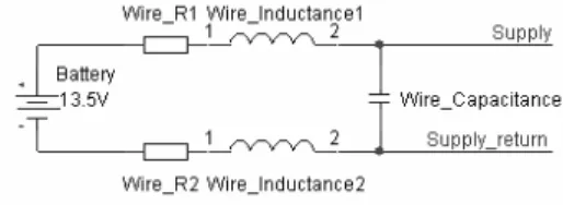
An electronic control unit [6] and its attached motor are connected with real wires to the battery/alternator supply system, which have finite resistance and parasitic inductance/capacitance. The resulting model (Figure 3) is used to simulate real behavior (e.g. oscillations in the cable harness).

Figure 3. Battery and connections model

The controlling element is a 6 transistor bridge (Figure 4), which must be driven in such a way that the motor receives the intended commands and that does not allow simultaneous switching of the high and low side transistors in the same inverter leg. This is implemented as a minimum dead time between transistor firing.

Figure 4. 6-transistor Inverter Bridge

IV. CONTROL TECHNIQUES

The driving technique is being implemented through software. For the PSpice simulation, a repeating pattern defined as a digital stimuli file control the transistor bridge.

The way of driving is being applied taking into account the type of application.[7]

The signals for the H Bridge are the PWM signals used to open the transistors. In real life and in case of simulations, the driver has to have implemented a dead time sequence between the turn-on of the phases in order to avoid damaging the transistors and in order to allow correct measurement of transferred power from the supply to the load.

PWM signals are being applied in the following way: High side PWM, low side full ON or OFF.

In order to avoid overheating the transistors, a switching technique between firing the high side with PWM and low side with full ON or OFF and inverse can be implemented.

A. 6-step PWM control

One possibility is using a 6 step PWM control technique (Figure 5), graphically described below:

Figure 5. 6-step control technique.

The switching pattern is the same for each of the 3 phases, but with a 120° offset.

In order to implement the technique in software the following have to be taken into account: at 6-step control, it is sufficient if the microcontroller receives an interrupt at every 60 electrical degrees to activate the next state of the bridge.

These interrupts usually are generated by hall sensors which indicate the real position of the rotor relative to the stator.

It is very advantageous for the implementation of various control method if the microcontroller recognizes the following five states:

 Bridge is inactive (tri-state, high impedance)

 Terminal connected to ground

 Terminal connected to supply

 Low Side PWM (If the duty cycle is equal to

100%, with ground connected)

 High Side PWM (If the duty cycle is equal to

100%, with supply connected)

By having the sensors on the motor, any kind of driving technique can be implemented; either rotational control or torque control.

In order to use the BLDC as a stepper motor, the Hall sensors are indispensable.

In order to drive the motor only rotational with no accurate control, the driving technique can be implemented without hall sensors.

For the implementation of the illustrated six-step commutation of the "Terminal 1" the following information has to be used in the driving procedure, and has to be stored somewhere (e.g. a look up table).

 330 ° -30 °: bridge inactive

 30 ° -90 °: high-side PWM

 90 ° -150 °: phase to supply

 150 ° -210 °: bridge inactive

 210 ° -270 °: low-side PWM

 270 ° -330 °: phase to ground

B. 12 Step PWM driving technique

The 12-step [2], [3] control driving technique needs an interrupt to the microcontroller at every 30 electrical degrees, in order to enable the next state of the bridge. These interrupts can be triggered either by six hall sensors, placed at 60 ° from each other or the same phenomena can be simulated by the microcontroller, by having simulated hall sensors which generate the additional required information for the driving technique. A 12 step control is graphically described below (Figure 6).

This technique is almost the same as the 6 step technique, the difference being that the switching time between the phases will be at 30° instead of 60°. This offers better control, leading to less vibrations of the motor and a more accurate driving when speaking of rotation speed and torque control.

In BLDC applications common problems are power losses, driving frequency and current ripple.

In order to implement BLDC motor control in a human related application we have to take into account the driving frequency as a starting point.

For many applications, it is usually between 21 kHz and 23 kHz (or lower if the risk of hearing the control cycle is also lower – e.g. if control unit is placed far from the driver), because these values are above human hearing range and allow fast enough reaction times from the control algorithm.

The higher the frequency of switching the better the current control we will have.

(11)

(12)

(13)

Figure 6. 12-step control technique.

All three legs of the inverter must have individual PWM duty cycles, dependent of the rotor angle. The duty cycle can be calculated using the below equation:

(14)

A proposed method in order to have a good current control is the Sinus Flat top modulation [5], [6], [7]. The voltages resulting by applying the duty cycle will have a quasi-sinus form. The final effect on the motor has to take into account the integration property due to the motor inductances. The phase voltages will be calculated as follows:

The maximum values of the duty cycle [6] will be written in a look up table and the value of the rotor angle and two other values, with 120° shift, read. All these values will be inputted in the above equation and the resulting PWM commands forwarded to the microcontroller PWM blocks and then to the inverter.

In order to change between 6 and 12 step control, only the values in the look up tables must be different. Choosing between one and the other is as simple as running a different initialization script.

V. CONCLUSION

(4)

(5)

(6)

Mathematical models and simulation models were built to study, improve and implement a control strategy for BLDC motors, with minimum hardware/software resources.

The supply voltage will be delivered by applying a

variable Duty cycle between 00% and 255100%

(with 8 bit PWM hardware units). The PWM step number and the extreme values are chosen after taking into account how fine the resulting control must be. For the next step we have to calculate the sinus voltage without the star null point:

By requiring two look up tables and minimal position information, the implementation of each driving technique is easy to use, relying on emulation of additional sensors and performing like more complicated solutions. The type of the application will allow deciding on the method to use.

VI. REFERENCES

[1] Michel, Robert. 2009. Kompensation von sättigungsbedingten Harmonischen in den Strömen feldorientiert geregelter Synchronmaschinen. Dresden : Vieweg + Teubner, 2009.

(7)

(8)

(9)

[2] Schröder, Dierk. 2009. Elektrische Antriebe - Regelung von Antriebssystemen. Berlin Heidelberg : Springer-Verlag, 2009.

Where U[1,2,3] in [V] is the calculated voltage value

without the zero value from star point connection at supply 1, 2 or 3. Also, we have to calculate the zero of the system:

[3] Tarmoom, Osama. 2006. Beitrag zur Auslegung von Permanent-Magnet-Motoren für spezielle Einsatzgebiete dargestellt am Beispiel einer Versuchsmaschine. Cottbus : s.n., 2006.

[4] AVR928: Scalar sensorless methods to drive BLDC motors.

(10)

[5] FCM8202 3-Phase Sinusoidal Brushless DC Motor Controler.

Where U123Null in [V] is the offset on the 3 phase

voltages. It must be added to the voltages calculated without the zero system:

[6] Diplomarbeit 1999 Dozent: L.Wobmann Diplomand: Patrick Fuhrer Hochschule für Technik und Architektur Bern Abteilung Elektrotechnik und Elektronik

Use of Artificial Neural Network for Testing Effectiveness of

Intelligent Computing Models for Predicting Shelf Life of

Processed Cheese

GOYAL Sumit, GOYAL Kumar Gyanendra

National Dairy Research Institute, Karnal -132001, India E-mail:[email protected]; [email protected]

Abstract – This paper presents the suitability of

artificial neural network (ANN) models for predicting the shelf life of processed cheese stored at 7-8ºC. Soluble nitrogen, pH; standard plate count, yeast & mould count, and spore count were input variables, and sensory score was output variable. Mean square error, root mean square error, coefficient of determination and Nash - sutcliffo coefficient were used in order to test the effectiveness of the developed ANN models. Excellent agreement was found between experimental results and these mathematical parameters, thus confirming that ANN models are very effective in predicting the shelf life of processed cheese.

Keywords: artificial neural network; artificial intelligence; processed cheese; prediction; shelf life; radial basis (exact fit)

I. INTRODUCTION

Processed cheese is a very popular variety of cheese. It is manufactured from 4 to 6 months old ripened grated Cheddar cheese. A part of ripened cheese is often replaced by fresh cheese.

During its preparation required amount of water, emulsifiers, extra salt, preservatives, food colorings and spices (optional) are added, and the mixture is heated to 70º C for 10-15 min with steam in a cleaned double jacketed stainless steel kettle (which is open, shallow and round-bottomed) with continuous gentle stirring (about 50-60 circular motions per minute) with a flattened ladle in order to get unique body & texture and desirable consistency in the product.

The determination of shelf life of processed cheese in the laboratory is very cumbersome and costly affair, and takes a very long time to give results.

Therefore, it was felt that ANN technique, which has been vastly applied for predicting the shelf life of various food products, be employed for processed cheese as well.

Hence, the present research was planned with the aim to develop feedforward ANN single and multilayer

intelligent models for predicting the shelf life of processed cheese stored at 7-8ºC.

The first Artificial Neural Network (ANN) was invented in 1958 by psychologist Frank Rosenblatt called perceptron. It was intended to model how the human brain processed visual data and learned to recognize objects.

An artificial neural network operates by creating connections between many different processing elements, each analogous to a single neuron in a biological brain.

These neurons may be physically constructed or simulated by a digital computer. Each neuron takes many input signals, then, based on an internal weighting system, produces a single output signal that's typically sent as input to another neuron. The neurons are tightly interconnected and organized into different layers.

The input layer receives the input; the output layer produces the final output [1]. A radial basis function network is an ANN that uses radial basis functions as activation functions. It is a linear combination of radial basis functions.

They are used in function approximation, time series prediction, and control. Radial basis function network consists of one layer of input nodes, one hidden radial-basis function layer and one output linear layer [2].

As an increasing number of new foods compete for space on supermarket shelves, the words “speed and innovation” have become the watchwords for food companies seeking to become “first to market” with successful products.

Overall quality of the product is of prime importance in this competitive market and needs to be built into the speed and innovation system. How the consumer perceives the product is the ultimate measure of food quality.

Therefore, the quality built in during the development and production process must last through the distribution and consumption stages.

the speed requirement, hence new accelerated studies have been developed [3]. The results of this research concerning development of radial basis (exact fit) ANN models for predicting the shelf life of processed cheese would be very beneficial for consumers, dairy factories manufacturing processed cheese, wholesalers, retailers, food researchers, academicians and regulatory authorities.

II. LITERATURE REVIEW

The literature survey revealed that the ANNs have been implemented for predicting the wide range of different physico-chemical characteristics of various food products including the quality and shelf life.

A. Fried Potato Chips

Quality of potatoes in chips industry is estimated from the intensity of darkening during frying. This is measured by a trained panel, subject to numerous factors of variation. Gray level intensities were obtained for the apex, the center, and the basal parts of each chip using image analysis of frying assays.

Feedforward ANN was designed and tested to associate these data with color categories. The developed ANN showed good performance, learning from a relatively small number of data values. The model behaved better than multiple linear regression analysis. Predicted categories appeared to reproduce the pattern of the experimental data issued from the trained panel, revealing nonlinear mapping, existence of sub regions and partial overlapping of categories.

Moreover, the generalization capacities of the network allowed to simulate plausible predictions for the whole set of parameter combinations.

Marique et al. (2003) were of the opinion that this

work is to be considered as a 1st _{step toward a practical}

ANN model that will be used for objective, precise, and accurate online prediction of chips quality [4].

B. Honey

Seventy samples of honey of different geographical and botanical origin were analyzed with an electronic nose. The instrument, equipped with 10 Metal Oxide Semiconductor Field Effect Transistors (MOSFET) and 12 Metal Oxide Semiconductor (MOS) sensors, was used to generate a pattern of the volatile compounds present in the honey samples.

The sensor responses were evaluated by Principal Component Analysis (PCA) and ANN. Good results were obtained in the classification of honey samples by using a neural network model based on a multilayer perceptron that learned using a backpropagation algorithm.

According to researchers methodology is simple, rapid and results suggested that the electronic nose could be a useful tool for the characterization and control of honey [5].

C. Beef

A series of partial least squares (PLS) models were employed to correlate spectral data from FTIR (Fourier Transform Infrared Spectroscopy) analysis with beef fillet spoilage during aerobic storage at different temperatures (0,5,10,15,and20ºC).

The performance of the PLS models was compared with a three - layer feedforward ANN developed using the same dataset. FTIR spectra were collected from the surface of meat samples in parallel with microbiological analyses to enumerate total viable counts.

Sensory evaluation was based on a three-point Hedonic scale classifying meat samples as fresh, semi-fresh, and spoiled. The purpose of the modelling approach employed in this work was to classify beef samples in the respective quality class as well as to predict their total viable counts directly from TIR spectra.

The results obtained demonstrated that both approaches showed good performance in discriminating meat samples in one of the three predefined sensory classes.

The PLS classification models showed performances ranging from 72.0 to 98.2% using the training dataset, and from 63.1 to 94.7% using independent testing dataset.

The ANN classification model performed equally well in discriminating meat samples, with correct classification rates from 98.2 to 100% and 63.1 to73.7% in the train and test sessions, respectively.

PLS and ANN approaches were also applied to create models for the prediction of microbial counts. The performance of these was based on graphical plots and statistical indices (bias factor, accuracy factor and root mean square error) [6].

D. Dairy products and sterilized drinks

Attention has been focused on the application of neural networks for developing different models for various dairy products and milk based sterilized drinks: Cakes [7]; soft cakes [8]; kalakand [9]; instant coffee drink [10]; instant coffee flavoured sterilized drink [11, 12]; milky white dessert jeweled with pistachio [13]; brown milk cakes [14]; soft mouth melting milk cakes [15]; post-harvest roasted coffee sterilized milk drink [16]; and processed cheese [17,18,19,20,21].

III. METHOD MATERIAL

The input variables used for developing the ANN computing models were the experimental data of processed cheese relating to soluble nitrogen, pH; standard plate count, yeast & mould count, and spore count; and sensory score assigned by the trained panelists was output variable (Fig.1). All in all 36 observations for each input and output variables were used for developing the models.

The dataset was randomly divided into two disjoint

validation set 6. Mean Square Error : MSE (1), Root Mean Square Error : RMSE (2), Coefficient of

Determination : R2 _{(3) and Nash - Sutcliffo Coefficient}

: E2 _{(4) were applied in order to compare the prediction}

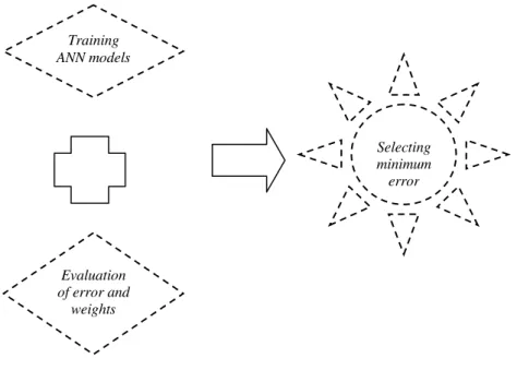
ability of the developed models. Training pattern of ANN models is illustrated in Fig. 2.

Sensory Score Standard

plate count Soluble nitrogen

pH

Yeast & mould count

Spore count

Figure1. Input and output parameters for ANN models.







































2

1 exp N

cal

n

Q

Q

MSE

(1)







































2

1 exp

exp

1

cal

Q

Q

Q

n

RMSE

(2)









































2

1 _exp2

exp

2

₁

Q

Q

Q

R

(3)











































2

1 exp exp

exp

2

₁

Q

Q

Q

Q

E

(4)

Where,

= Observed value;

exp

Q

= Predicted value;

cal

Q

=Mean predicted value;

exp

Q

= Number of observations in dataset.

Figure 2. Training pattern for ANN network.

IV. RESULTS AND DISCUSSION

ANN model’s performance matrices for predicting the sensory scores are presented in Table 1.

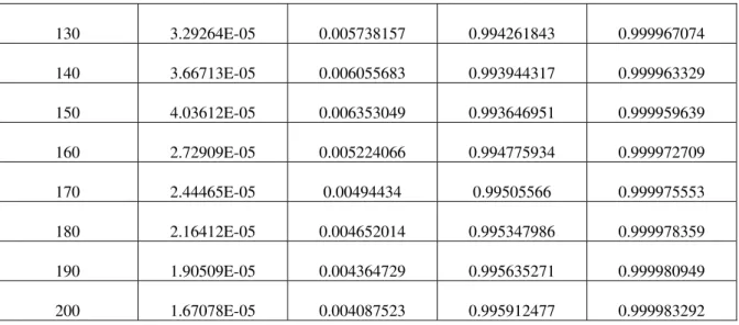
Table 1. Results of Radial Basis (Exact Fit) model.

Spread Constant MSE RMSE R2 E2

10 0.002660019 0.051575367 0.948424633 0.997339981

20 0.002422522 0.04921912 0.95078088 0.997577478

30 0.001958471 0.044254619 0.955745381 0.998041529

40 0.001767319 0.042039494 0.957960506 0.998232681

50 0.002009656 0.04482919 0.95517081 0.997990344

60 1.04864E-05 0.003238266 0.996761734 0.999989514

70 8.32216E-07 0.000912259 0.999087741 0.999999168

80 7.6146E-06 0.002759456 0.997240544 0.999992385

90 1.44227E-05 0.003797717 0.996202283 0.999985577

100 2.00537E-05 0.004478131 0.995521869 0.999979946

110 2.48217E-05 0.004982141 0.995017859 0.999975178

120 2.90291E-05 0.005387869 0.994612131 0.999970971

Selecting minimum error

Evaluation of error and

130 3.29264E-05 0.005738157 0.994261843 0.999967074

140 3.66713E-05 0.006055683 0.993944317 0.999963329

150 4.03612E-05 0.006353049 0.993646951 0.999959639

160 2.72909E-05 0.005224066 0.994775934 0.999972709

170 2.44465E-05 0.00494434 0.99505566 0.999975553

180 2.16412E-05 0.004652014 0.995347986 0.999978359

190 1.90509E-05 0.004364729 0.995635271 0.999980949

200 1.67078E-05 0.004087523 0.995912477 0.999983292

Radial Basis (Exact Fit) model was developed for predicting the shelf life of processed cheese stored at

7-8o _{C. The comparison of Actual Sensory Score (ASS)}

and Predicted Sensory Score (PSS) for Radial Basis (Exact Fit) model is illustrated in Fig. 3. Radial Basis

(Exact Fit) model with spread constant 70 [MSE:

8.32216E-07; RMSE: 0.000912259; R2_{: 0.999087741;}

E2_{:0.999999168] gave the best fit amongst all the}

studied experiments (Table 1).

Figure 3. Input and output parameters for ANN models.

The modeling results showed that there was excellent agreement between the experimental data and predicted values, with a high determination coefficient

(R2 _{= 0.999087741) and Nash - Sutcliffo Coefficient (E}2

= 0.999999168) showing that the developed model was able to analyze nonlinear multivariate data with very

good performance. It is evident from the high R2 _{and E}2

that the ANN computing models are very effective in predicting the shelf life of processed cheese.

V. CONCLUSIONS

An effective new radial basis (exact fit) method based on artificial neural network is proposed for predicting the shelf life of processed cheese stored at

7-8o _{C. The results were verified by comparing them with}

laboratory observations by employing mean square error, root mean square error, coefficient of determination and Nash - sutcliffo coefficient. Very good correlation was found between experimental data and the developed mathematical models, thus confirming the suitability of radial basis (exact fit) artificial neural networks for predicting the shelf life of processed cheese.

REFERENCES

[1] http://www.computerworld.com/s/article/57545/Artificial _Neural_Networks (accessed on 11.1.2011).

carbonarius using neural networks”, Journal of Applied Microbiology, vol.107, no.3, pp. 915-927, 2009.

[3] Medlabs Website:

http://www.medlabs.com/Downloads/food_product_shelf_ life_web.pdf (accessed on 1.3.2011).

[4] T. Marique, A. Kharoubi, P. Bauffe and C. Ducattillon, “Modeling of fried potato chips color classification using image analysis and artificial neural network”, Journal of Food Science, vol.68, no.7, pp. 2263-2266, 2003.

[5] S. Benedetti, S. Mannino, A.G. Sabatini and G.L Marcazzan,”Electronic nose and neural network use for the classification of honey,” Apidologie, vol.35, pp. 1–6, 2004. [6] Z.P. Efstathios, R.M. Fady, A.A. Argyria, M.B. Conrad

and E. N. George-John, ”A comparison of artificial neural networks and partial least squares modelling for the rapid detection of the microbial spoilage of beef fillets based on Fourier transform infrared spectral fingerprints”, Food Microbiology, vol.28, no.4, pp. 782–790, 2011.

[7] Sumit Goyal and G.K. Goyal, ”Brain based artificial neural network scientific computing models for shelf life prediction of cakes”, Canadian Journal on Artificial Intelligence, Machine Learning and Pattern Recognition, vol. 2, no. 6, pp.73-77, 2011.

[8] Sumit Goyal and G.K. Goyal, ” Simulated neural network intelligent computing models for predicting shelf life of soft cakes”, Global Journal of Computer Science and Technology, vol.11, no.14, version 1.0, pp. 29-33, 2011. [9] Sumit Goyal and G.K. Goyal, ”Advanced computing

research on cascade single and double hidden layers for detecting shelf life of kalakand: An artificial neural network approach”, International Journal of Computer Science & Emerging Technologies, vol.2, no.5, pp. 292-295, 2011.

[10]Sumit Goyal and G.K. Goyal, ”Application of artificial neural engineering and regression models for forecasting shelf life of instant coffee drink”, International Journal of Computer Science Issues, vol. 8(4), no. 1, pp. 320-324, 2011.

[11]Sumit Goyal and G.K. Goyal, ” Cascade and feedforward backpropagation artificial neural networks models for prediction of sensory quality of instant coffee flavoured sterilized drink”, Canadian Journal on Artificial Intelligence, Machine Learning and Pattern Recognition, vol.2, no.6, pp.78-82, 2011.

[12]Sumit Goyal and G.K. Goyal, ”Development of neuron based artificial intelligent scientific computer engineering

models for estimating shelf life of instant coffee sterilized drink”, International Journal of Computational Intelligence and Information Security, vol.2, no.7, pp. 4-12, 2011. [13]Sumit Goyal and G.K. Goyal, ” A new scientific approach

of intelligent artificial neural network engineering for predicting shelf life of milky white dessert jeweled with pistachio”, International Journal of Scientific and Engineering Research, vol.2,no.9, pp. 1-4, 2011.

[14]Sumit Goyal and G.K. Goyal, ”Radial basis artificial neural network computer engineering approach for predicting shelf life of brown milk cakes decorated with almonds”, International Journal of Latest Trends in Computing, vol.2,no.3, pp. 434-438, 2011.

[15]Sumit Goyal and G.K. Goyal, ”Development of intelligent computing expert system models for shelf life prediction of soft mouth melting milk cakes”, International Journal of Computer Applications, vol.25, no.9, pp. 41-44, 2011.

[16]Sumit Goyal and G.K. Goyal, “Computerized models for shelf life prediction of post-harvest coffee sterilized milk drink”, Libyan Agriculture Research Center Journal International, vol.2 , no.6, pp. 274-278, 2011.

[17]Sumit Goyal and G.K. Goyal, “Radial basis (exact fit) and linear layer (design) ANN models for shelf life prediction of processed cheese”, International Journal of u- and e- Service, Science and Technology, vol.5, no.1, pp.63-69, 2012.

[18]Sumit Goyal and G.K. Goyal, “A novel method for shelf life detection of processed cheese using cascade single and multi layer artificial neural network computing models”, ARPN Journal of Systems and Software, vol.2, no.2, pp.79-83, 2012.

[19]Sumit Goyal and G.K. Goyal, “Time – delay simulated artificial neural network models for predicting shelf life of processed cheese”, International Journal of Intelligent Systems and Applications, vol.4, no.5, pp.30-37, 2012. [20]Sumit Goyal and G.K. Goyal, “Estimating processed

cheese shelf life with artificial neural networks. International Journal of Artificial Intelligence (IJ-AI), vol. 1, no.1, pp.19-24, 2012.

A Z-Source Inverter for an Integrated Starter Alternator

HANGIU Radu-Petru, FILIP Andrei-Toader, MAR I

Ș

Claudia Stelu a,

BIRÓ Károly Ágoston

Technical University of Cluj-Napoca, Romania,

Department of Electrical Machines and Drives, Faculty of Electrical Engineering, Memorandumului, 28, 400114, Cluj-Napoca, Romania, E-Mail: [email protected]

Abstract –This paper presents an overview of an integrated starter alternator system used in mild hybrid electric vehicles. Inverter configurations that are used in HEV are assessed with an emphasis on the novel Z-source inverter topology. The final part presents a simulation model of a bi-directional Z-source inverter, developed in AMESim, and the simulation results.

Keywords: ISA; model; simulation; Z-source, AMESim.

I. INTRODUCTION

The conventional internal combustion engine (ICE) era is at its dawn because of the increase in fuel prices and a more stringent legislation on greenhouse gas emissions. The obvious alternative for personal transportation is the electric vehicle, but the technology needed to make this type of vehicles accessible to the masses is still at an initial stage. The hybrid electric vehicle (HEV) is a viable compromise until more efficient batteries or fuel cells are developed.

The HEV comes in different configurations. Depending on the power flow within the vehicle and on the energy sources, they can be classified as: series, parallel, series-parallel or as mild HEVs. The mild HEV configuration represents the first step in the transition from an ICE vehicle to a full HEV and onwards to a full electric vehicle. The integrated starter-alternator (ISA) unit represents the key difference between an ICE vehicle and a mild HEV.

The ISA is in fact an electric machine that has a two quadrant operation thus combining in one unit the starter and the alternator of a conventional ICE vehicle. Besides its main function of cranking the ICE and generating electric power, the ISA can be used to implement other functionalities that may improve fuel efficiency and ride comfort, such as: start/stop functionality, power boosting and regenerative braking.

The ISA is driven by a power converter which, in a conventional system, is composed of an inverter and a buck DC-DC converter. The inverter steps up the voltage of the battery and provides AC to the motor and the buck converter steps down the rectified voltage in order to charge the battery when the ISA is in generator mode.

The traditional inverter configurations used for HEV are the voltage source inverter (VSI) and the current

source inverter (CSI). The VSI has the advantage of a low cost and a simple control but has important drawbacks such as the necessity of a bulky dc bus capacitor, high electromagnetic noises, high frequency losses and the necessity of a separate dc-dc converter in order to boost the battery voltage. The CSI main advantage comes from its capability to boost the dc voltage of the battery without a separate boost converter. Other advantages come from the fact that it can withstand short circuits across any two of its output terminals, it doesn’t need a bulky dc bus capacitor or anti-parallel diodes thus reducing the overall size of the inverter. CSI disadvantages are the inability to reverse the DC current in order to charge the battery, high conduction losses and the need for forced commutation which means that only switches capable of blocking voltage in both directions can be used.

The Z-source (impedance source) inverter (ZSI) is a novel inverter configuration, first proposed by F. Z. Peng [1], that overcomes some of the limitations of traditional inverters.

This paper presents an application of a ZSI for a permanent magnet synchronous motor ISA to be used in a mild HEV. First the ISA architecture and ZSI are presented in detail. The final part presents simulation results of the ISA driven by a ZSI.

II. ISA SYSTEM OVERVIEW

As mentioned before, a vehicle equipped with an ISA is in fact a mild HEV. The main difference between a mild HEV and a full HEV comes from the fact that in the case of the mild HEV, the ICE is always on and is driving the wheels as long as the vehicle is moving.

A. Drive train configuration

There are several possible arrangements within the vehicle drive train for the electric machine acting as an ISA [2]:

• Classic arrangement

• Coaxial arrangement

• Non-coaxial arrangement

• Electric motor in auxiliary drive

• Electric motor in the transmission

two clutches and one with the machine mounted on the input shaft of the transmission. Similar arrangements are possible in the case of the non-coaxial solution where the electric machine that is now mounted on the side of the drive train will be connected via a drive.

The most widespread solution is that with the electric machine mounted on the crankshaft. The rotor is attached directly to the ICE’s crankshaft and replaces the flywheel. The advantage of such an arrangement, besides its simplicity, consists in achieving a dual mass flywheel effect by connecting the electric machine to the friction plate for the clutch, with a torsion damper. This will eliminate excessive transmission gear rattle, reduce gear shift effort and further increase fuel economy.

B. Operation modes

The ISA’s main function is to generate power while the ICE is on but it can also assist the engine when high loads are requested. The system’s modes of operation are:

1) Internal combustion engine cranking

2) Power generation mode

3) Regenerative braking mode

4) Power boost mode

C. Electric machines

For functioning as both a starter and an alternator the electric machine must have a wide constant power speed range. It must provide a high starting torque for engine cranking even at very low temperatures and it must have a high efficiency in generator mode at speeds ranging from 1500 rpm to 4000 rpm. At the moment the two competing electric machines for ISA applications are the Permanent Magnet Synchronous Machine (PMSM) and the Induction Machine (IM).

III. Z-SOURCE INVERTER

The Z-Source inverter, shown in Fig. 1, replaces the dc-link present in a conventional VSI with an impedance network composed of two capacitors and two inductors. This enables the inverter to utilize the shoot-through (short circuit) states of the phase legs in order to boost the dc-bus voltage. By varying the active state and shoot-through duty ratios, the ZSI can either buck or boost the dc-bus voltage.

A. Control methods

In order to utilize the shoot-through states the pulse width modulation (PWM) control used for conventional inverters needs to be modified. Several control methods have been proposed:

1) Simple boost control (SBC)

This method was first proposed in [1] and it utilizes an upper and a lower limit to control the shoot-through states. When the triangular carrier wave is greater than the upper limit, or lower than the lower limit, the inverter is in shoot-through state, the rest of the time the control is the same as a normal carrier-based PWM. This method’s disadvantage is the high voltage stress on the switches.

Figure 1. Z-Source inverter.

2) Maximum boost control (MBC)

This method was presented in [3]. Its working principle is to turn all of the inverter’s zero states into shoot-through states thus minimizing the voltage stress on the switches

Its main draw back is that it produces low frequency ripples across the Z-network because of the variable shoot-through duty ratio.

3) Maximum constant boost control (CBC)

This control method was proposed in [4]. The drawbacks of the previous two methods are mitigated by keeping a constant shoot-through duty ratio while maximizing the boost factor. This is achieved either by utilizing a variable lower and upper limit for controlling the shoot-through states, either by injecting a third-harmonic component into the reference signals. The envelopes used in the first case are periodic signals that have a frequency three times higher than that of the inverter output. The injected third harmonic component is 1/6 of the fundamental component. When using third harmonic injection the upper and lower limits for controlling the shoot-through states are straight lines. The distance between this two limits is constant and

equal to

3

M

B. Component rating

The inverter’s boost factor B and gain G can be

determined using the following [4]:

1 3

1

 

M

B (1)

1 3 2

/   



M M MB E

V G

S

m ₍₂₎

Where Vm is the peak phase output voltage, M is the

modulation index and ES is dc-bus voltage.

For rating the ZSI’s inductors and capacitors, for any control strategy, the following equations can be used [5]:



cos 3

1 ( 2

m i

S S S

MI k

d T d E

L  S) ₍₃₎

)

1

(

8

m S S

E

k

C





3

cos

S

d

MI

T

d



(4)

Where dSis the shoot-through duty ratio, kv and ki are

desired voltage and current ripple factors, Im is the peak

Figure 2. Control model.

C. DC-DC converter

In order to accept a reverse power flow from the ISA to the battery, a current fed Z-source dc-dc converter, proposed in [5] and [6] has been adopted.

This converter consists of a bi-directional switch, composed of two IGBTs and two diodes, a second switch and an inductor placed between the Z network and the 3 phase bridge and a smoothing capacitor. The bi-directional switch replaces the Z-source network diode so that, depending on the desired operating mode, the converter can now accept a direct or a reverse power flow. This converter can perform either as a buck converter, either as a reversed polarity buck-boost converter depending on the duty ratio.

By controlling the duty ratio of the switches the converter output voltage can be regulated. The voltage transfer ratio of the converter is determined with the following equation [6]:

D D

G2 1 (5)

Where G is the voltage gain and D is the duty ratio.

IV. SYSTEM MODELING AND SIMULATION RESULTS

The system model has been implemented in AMESim, which is a multi-domain simulation software for the modeling and analysis of one-dimensional (1D) systems.

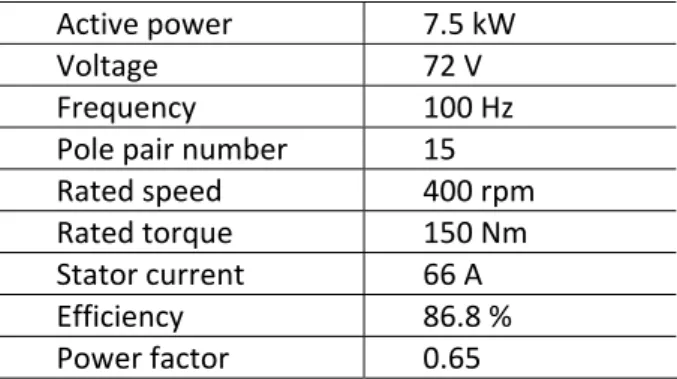
The chosen electric machine is a three-phase, 7.5 kW, outer rotor PMSM presented in [7]. The outer rotor configuration allows for an easy integration of the machine in the vehicle drive train and also helps with the cooling of the permanent magnet rotor. The electric machine specifications are:

Table 1. Electric machine specifications.

Active power  7.5 kW 

Voltage  72 V 

Frequency  100 Hz 

Pole pair number  15  Rated speed  400 rpm  Rated torque  150 Nm  Stator current  66 A 

Efficiency  86.8 % 

Power factor  0.65 

The battery dc voltage (ES) is set at 12 V, the inverter

switching frequency (TS) at 9 kHz and the voltage (kv)

and current (ki) ripple factors are 5% and 1%,

respectively. Considering the electric machine’s rated voltage and the battery’s voltage the inverter must

provide a voltage gain (G) of 6. The modulation index M

is 0.621.

Based on this values the Z-network inductance and capacity are determined using (3) and (4). The calculated values are:

H

L54.1 (6)

mF

C3.9 (7)

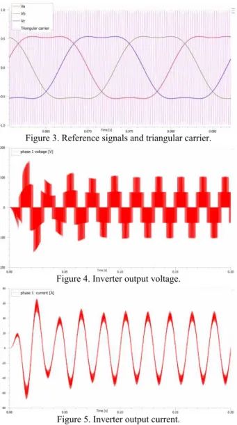
Figure 3. Reference signals and triangular carrier.

Figure 4. Inverter output voltage.

Figure 5. Inverter output current.

Fig. 3 shows the reference signal with the injected third harmonic component and the triangular carrier signal.

Fig. 4 and Fig. 5 present the inverter output voltage and current waveforms. The peak output voltage is 104 V and the peak output current is 87 A.

V. CONCLUSIONS

The Z-source inverter is a novel inverter topology that overcomes some of the limitations of conventional inverters. Coupled with a Z-source dc-dc converter, the

Z-source inverter can be used as the power converter for an ISA system.

This paper first presents the ISA system configuration followed by a description of the Z-source inverter.

The Z-network components are rated and a simulation is carried out in order to confirm the system’s expected behavior. The Z-source inverter is a suitable candidate for driving the ISA in a mild HEV. By combining the Z-source inverter with a Z-source dc-dc converter the system’s complexity is reduced and the resulting converter can perform either as a buck or as a boost converter.

ACKNOWLEDGMENT

This paper was supported by the project

"Improvement of the doctoral studies quality in

engineering science for development of the knowledge based society-QDOC" contract no. POSDRU/107/1.5/ S/78534, project co-funded by the European Social Fund through the Sectorial Operational Program Human Resources 2007-2013.

REFERENCES

[1] F. Z. Peng, “Z-source inverter”, IEEE Trans. Ind. Appl., vol. 39, no. 2, pp. 504-510,Mar./Apr. 2003.

[2] W. Reik, “Electrical Motor in the Drive Train”, LuK GmbH & Co. KG technical presentation, pp. 3-8, Apr. 2004.

[3] F. Z. Peng, M. Shen, and Z. Qian, “Maximum boost

control of the Z-source inverter”, IEEE Trans. Power Electron., vol. 20, no. 4, pp. 833-838,Jul./Aug. 2005. [4] M. Shen, J. Wang, et al., “Constant boost control of the

Z-source inverter to minimize current ripple and voltage stress”, IEEE Trans. Ind. Appl., vol. 42, no. 3, pp. 770-777, May/Jun. 2006.

[5] S. Rajakaruna, and B. Zhang, “Design and control of a bidirectional Z-source inverter”, in Proc. IEEE Power Eng. Conf., 2009.

[6] X. Fang, “A novel Z-source DC-DC converter”, in Proc. IEEE International conference on Industrial Technology 2008, pp. 1-4, Apr. 2008.

Bearing Faults Condition Monitoring – A Literature Survey

HARLI

Ş

CA Ciprian, SZABÓ Loránd

Department of Electrical Machines and Drives, Technical University of Cluj-Napoca 400114 Cluj-Napoca, Memorandumului 28, Romania; e-mail: [email protected]

Abstract – Bearing related faults are one of the most common causes of failure in electrical machines. By means of advanced diagnosis methods it is possible to detect these faults in their incipient phase, before the catastrophic effects of the failures can occur. The aim of this paper is to make a brief survey of the condition monitoring techniques used in the field of bearing fault diagnosis.

Keywords: bearing faults, diagnosis, induction

machines, fault detection, condition monitoring.

I. INTRODUCTION

In most industrial processes unplanned stops due to failures have a high economic impact on the cost of the process and it may result in significant process down time. The fault can occur in any part of the machine or even in the drive system. The faults of electrical machine could be electrical or mechanical. The main electrical faults are the stator and rotor windings (or cage) faults [1], [2]. Mechanical faults include bearing faults, air-gap eccentricity, misalignment, gearboxes faults, etc.

The research on fault diagnosis has shown that the most of the failures of induction machines (about 40%) are related to the bearings [3]. The bearing related faults do not cause immediate breakdown, they evolve in time until they produce a critical failure of the machine. Unfortunately these failures results both in costly repair and downtime.

The bearings faults can be caused by material fatigue, overheating, harsh environments, inadequate storage, contamination, corrosion, wrong handling and installation, etc. But the main cause of their failure is due to poor lubrication, which can be easily avoided by a correct maintenance plan.

Vibration based monitoring techniques are usually applied for the diagnosis of the bearings. Unfortunately these methods require vibration sensors and special equipment for the condition monitoring. They also need access to the machine under testing, which is not always possible.

Compared to the methods above, the current monitoring requires only (frequently already existing) simple and cheap current sensors.

The current monitoring based techniques can be used to detect a large number of faults: broken rotor bars [4] [5], shorted windings, air-gap eccentricity [6], bearing faults [7], load faults, etc.

These methods are non-intrusive and can be applied both on-line and in a remotely controlled way.

II. BEARING FAULTS

A rolling-element bearing is generally composed of two rings, between which a set of balls or rollers rotate in raceways. In most cases, bearing failures are the result of material fatigue of the bearing. Under normal operating conditions fatigue failure begins with small cracks, located inside the surfaces of the raceway and rolling elements.

The repetitive impacts between the components of the bearing and the faulted surfaces cause the cracks to gradually propagate and expand, generating an increase in vibrations and noise levels [8].

The repetitive stressing of the damaged area causes the detachment of some small fragments of the material, which produce a phenomenon known as flaking or spalling [9]

The pattern of the vibration signal consists in a succession of oscillations which repeat with each pass of a moving component over the fault [10]. The repetition frequency of the impact depends on the position of the fault. The fault can be on the inner race, the outer race or on the rolling element

The typical construction and sizes of a ball bearing is shown in Fig. 1. The balls are fixed and held together by a cage which prevents the contact between the balls and ensures a uniform distance between them.

Figure 1. Main bearing dimensions and characteristic fault frequencies [1].

 the location of the fault: inner race, outer race, balls, and cage [7].

 the fault signature: single-point defects and

generalized roughness [11].

A. SINGLE-POINT DEFECTS

A single-point defect can produce different characteristic fault frequencies in the vibration spectrum of the machine. These frequencies are predictable and depend on the surface of the bearing which contains the fault [12].

The single-point defects cause periodic impulses in vibration signals. Amplitude and period of these impulses are determined by shaft rotational speed, fault location and bearing dimensions. Therefore, a specific frequency can be attributed to each component of the bearing [13].

The fundamental cage frequency is given by:

 

 1 cos

2 D

d f

fc r (1)

The ball defect, respectively the inner race defect frequencies can be computed by using the following equations:

 

 2 

2 2 cos 1 D d f d D

fbd r (2)





 

 1 cos

2 D d nf f f n f r c r

id (3)

The formula for computing the outer race defect frequencies is the following:

 

 1 cos

2 D d d nf nf f r c

od (4)

where, fr is the rotor speed, n the number of balls, d the

diameter of the ball, D the pitch diameter of the bearing

and α the contact angle as shown in Fig. 1. The typical

value of the contact angle is 0°.

For most bearings with six to twelve balls, the frequencies given by (3) and (4) can be approximated with [13]:

r

id n f

f 0.6  (5)

r

od n f

f 0.4  (6)

It is known that any air-gap eccentricity produces anomalies in the air-gap flux density, which is reflected on the stator current. In the case of a bearing fault the characteristic fault frequencies are modulated by the electrical supply frequency at a predictable frequency [13].

V s

bng f m f

f    (7)

where fs is the electrical supply frequency, fV one of the

fault frequencies defined by equations (1)÷(4) and

m = 1, 2, 3...

B. GENERALIZED ROUGHNESS FAULT

Generalized roughness fault is the most frequent cause of bearing failure. It usually occurs in the industrial environment due to various causes such as [12]:

 Lack or loss of the lubricant, contamination of

lubricant

 Misalignment

 Shaft currents

 Environmental conditions (dust, water, acid and

humidity).

 Bearing corrosion, produced by the presence of

water and acids.

These causes lead to a faster wear of components of the bearing, especially raceways and balls. They to produce generalized roughness fault, as well as single-point defects. A generalized roughness fault of a bearing can be easily determined because it spins roughly or with some difficulty.

III. CONDITION MONITORING OF BEARING FAULTS

A significant part of the papers on the fault diagnosis of induction machines are dealing with on the faults of rolling bearings.

Even though that vibration based condition monitoring techniques are usually applied for the diagnosis of the bearings, many papers use the stator current analysis, due to its advantages.

The methods used for stator current analysis decompose and analyze the signal using various techniques such as Fourier analysis, neural networks, wavelets, statistical analysis, etc.

In [14] the authors analyze two types of bearing faults: a hole drilled into the outer raceway and an indentation produced in the inner and outer surface. Vibration and current analysis is applied to both faulty conditions.

The specific characteristic fault frequencies are highlighted for both faults. The analysis of the first fault

shows two components, fod and 2fod in the vibration

spectrum, and |fs ± fod| and |fs ± 2fod| in the current

spectrum. For the second type of fault the highlighted

characteristics are fod, 2fod and fid for the vibration

spectrum, and |fs ± fod|,|fs ± 2fod| and |fs ± fid|, for the current spectrum.

In [27] the authors introduce a new formulation for the current spectral analysis for the detection of bearing failures in induction motors driven by frequency power converters. The fault is an outer race defect and the authors highlight an increase of the specific fault frequencies components of the current spectrum.

realigning the test motor can alter the vibration and current spectra.

Some authors studied the detection of faults in electrical machines by using the stray flux around the motor [17], [18], [19], [20], [21], [22].

In [20] a small active area sensor was used for the detection of eccentricity and bearing faults. For the bearing fault analysis, a hole was drilled in the inner race of the bearing. Current and stray flux measurements were effectuated under different loading conditions. The spectra of the signals were obtained using Fast Fourier Transform (FFT). The characteristic fault frequencies were almost the same in both spectra, current and flux, but the amplitudes of these components were low in both cases.

In [16] the Park's Vector Approach is used for the detection of broken bearings. The analysis is made on a four bearings with drilled holes in the inner race and outer race. One of the bearings has two drilled holes in the outer race. The authors concluded that the diagnosis of the inner race faults is more difficult because of vibration signal is weak and it is not fully transmitted to the outer race. The results show a good detection of the faulty conditions.

The Park's Vector Approach was also used in [23] for the diagnosis of three bearings with different diameter holes in the outer race. The proposed method showed good results in detecting even an incipient fault can be detected using this method. This paper also presents a new technology for artificially introducing bearing faults such as: pitting, flutting or false brinelling. The method consists in removing the pins of the cage, so all the bearing components can be accessible.

In [24] the Continuous wavelet transform (CWT) is used for the extraction of characteristic features from vibration signals measured for induction machines subjected to bearing fluting. The faults of the bearing were obtained artificially by using an Electrical Discharge Machining (EDM) and thermal ageing. The proposed method was compared with Short-Time Fourier Transform and it was highlighted that the CWT has some advantages. By using the CWT the authors were able extract small amplitudes that cannot be observed along the frequency axis. Also, they found

extra amplitudes caused by the damage of the bearing between 2÷4 kHz.

In [25, 26] the broken bar and bearing faults (inner race defect) of several inverter-fed induction machines are studied with a new hybrid algorithm that combines the analysis of the signal in time and frequency domain. This new method uses a combination between Independent Component Analysis (ICA) and FFT in order to analyze features of the stator current. ICA is a statistical technique for decomposing a complex dataset into independent subparts. The authors state that proposed method detects and classifies correctly the characteristic fault frequency components. In the case of bearing faults, the detection is more difficult. It is shown that the predominant characteristic fault frequency is

given by fid

For bearing fault diagnosis other authors have used different methods such as: neural networks [28], hidden Markov modeling [29], instantaneous power factor [30], etc.

Figure 2. Example of artificially drilled holes in the outer raceway of a bearing [16].

IV. CONCLUSIONS

The literature reviewed in this paper aims to investigate the possibility of employing the analysis of the stray flux and stator current for bearing fault detection of induction machines in future papers.

ACKNOWLEDGMENT

This paper was supported by the project

"Improvement of the doctoral studies quality in

engineering science for development of the knowledge based society-QDOC" contract no. POSDRU/107/1.5/ S/78534, project co-funded by the European Social Fund through the Sectorial Operational Program Human Resources 2007-2013.

REFERENCES

[1] W.T. Thomson, "A review of on-line condition

monitoring techniques for three-phase squirrel-cage induction motors – Past present and future," Proceedings of the IEEE Symposium on Diagnostics for Electrical Machines, Power Electronics and Drives (SDEMPED '99), Gijon (Spain), pp. 3-18, 1999.

[2] M.E.H. Benbouzid, "A review of induction motors signature analysis as a medium for faults detection," IEEE Transactions on Industrial Electronics, vol. 47, no. 5 (October 2000), pp. 984-993, 2000.

[3] Motor Reliability Working Group, "Report of large motor reliability survey of industrial and commercial installations Part I and II," IEEE Transactions on Industry Applications, vol. IA21, no. 4 (July 1985), pp. 853-872, 1985.

[4] F. Filippetti, G. Franceschini, C. Tassoni, "Neural networks aided online diagnostics of induction motor rotor faults," IEEE Transactions on Industry

Applications, vol. 31, no. 4 (July-August 1995),

pp. 892-899, 1995.