Working
Paper
330
Semiparametric estimation
and inference using doubly
robust moment conditions
Christoph Rothe
Sergio Firpo
CMICRO - Nº15
Os artigos dos Textos para Discussão da Escola de Economia de São Paulo da Fundação Getulio
Vargas são de inteira responsabilidade dos autores e não refletem necessariamente a opinião da
FGV-EESP. É permitida a reprodução total ou parcial dos artigos, desde que creditada a fonte.
Escola de Economia de São Paulo da Fundação Getulio Vargas FGV-EESP
Semiparametric Estimation and Inference Using Doubly
Robust moment conditions
Christoph Rothe and Sergio Firpo∗
Abstract
We study semiparametric two-step estimators which have the same structure as
para-metric doubly robust estimators in their second step. The key difference is that we do not
impose any parametric restriction on the nuisance functions that are estimated in a first
stage, but retain a fully nonparametric model instead. We call these estimators
semipara-metric doubly robust estimators (SDREs), and show that they possess superior theoretical
and practical properties compared to generic semiparametric two-step estimators. In
par-ticular, our estimators have substantially smaller first-order bias, allow for a wider range
of nonparametric first-stage estimates, rate-optimal choices of smoothing parameters and
data-driven estimates thereof, and their stochastic behavior can be well-approximated by
classical first-order asymptotics. SDREs exist for a wide range of parameters of interest,
particularly in semiparametric missing data and causal inference models. We illustrate our
method with a simulation exercise.
JEL Classification: C14, C21, C31, C51
Keywords: Semiparametric estimation, missing data, treatment effects, double robustness
∗This Version: December 20, 2012. Christoph Rothe, Columbia University, Department of Economics, 420 W
1. Introduction
Semiparametric models are of great importance for applied econometric research. These models
often imply that the finite-dimensional parameter of interest can be characterized through a
moment condition containing an unknown nuisance function. This structure then leads to
a two-step semiparametric estimation approach. In the first step, the nuisance function is
estimated nonparametrically. In the second step, the parameter of interest is estimated from
an empirical version of the moment condition, with the unknown nuisance function replaced
by its first-step estimate. These estimators are used in a wide range of applications, and their
theoretical properties have been studied extensively (e.g. Newey, 1994; Newey and McFadden,
1994; Andrews, 1994; Chen, Linton, and Van Keilegom, 2003; Ichimura and Lee, 2010).
In this paper, we consider semiparametric two-step estimators that are based on a moment
condition that exhibits a particular structure: it depends on two unknown nuisance functions,
but still identifies the parameter of interest if either one of the two functions is replaced by some
arbitrary value. Following Robins, Rotnitzky, and van der Laan (2000) and Robins and
Rot-nitzky (2001), we refer to such moment conditions asdoubly robust, and call the corresponding
estimatorssemiparametric doubly robust estimators (SDREs). These estimators differ from the
usual doubly robust procedures used widely in statistics (e.g. Van der Laan and Robins, 2003),
which rely on additional parametric restrictions on the nuisance functions. Our main
contri-bution is to show that a SDRE possesses several attractive theoretical and practical properties
relative to a generic semiparametric two-step estimator, even if the two are first-order
asymp-totically equivalent. In particular, SDREs are generally root-n-consistent and asymptotically normal under weaker conditions on the smoothness of the nuisance functions, or, equivalently,
on the accuracy of the first step nonparametric estimates, and their stochastic behavior can thus
be better approximated by classical first-order asymptotics. In practice, this means that SDREs
generally have smaller first-order bias, are more invariant with respect to the implementation
of the nonparametric first stage, allow for rate-optimal choices of smoothing parameters and
data-driven estimates thereof, and do not require the use of bias reducing nonparametric
esti-mators (such as those based on higher-order kernels) in settings with moderate dimensionality.
SDREs are also adaptive, in the sense that by construction their asymptotic variance does not
calculation of standard errors.
Doubly robust moment conditions are known to exist for many interesting parameters in a
wide range of semiparametric models, including regression coefficients in models with missing
outcomes and/or covariates (e.g. Robins, Rotnitzky, and Zhao, 1994; Robins and Rotnitzky,
1995), average treatment effects in potential outcome models with unconfounded assignment
(Scharfstein, Rotnitzky, and Robins, 1999), and local average treatment effects in instrumental
variable models (Tan, 2006), amongst many others. Such results can thus readily be used to
construct our SDREs. In all the aforementioned examples, and several others, a doubly robust
moment condition takes the form of an expectation of the respective efficient influence (or
“score”) function, and thus SDREs are semiparametrically efficient in these settings (Newey,
1994). SDREs therefore have favorable properties even compared to other efficient estimators
that are commonly used in such settings, such as e.g. Inverse Probability Weighting estimators
in missing data and treatment effect models (e.g. Hirano, Imbens, and Ridder, 2003; Chen,
Hong, and Tarozzi, 2008).
As mentioned above, doubly robust moment conditions are traditionally used in connection
with fully parametric specifications for each of the two nuisance functions, as this ensures that
the resulting estimator is consistent if at least one of the parametric specifications is correct.
The use of parametric doubly robust estimators is typically motivated by valid concerns about
the reliability of semiparametric two-step estimators, especially the accuracy of conventional
approximations of their finite sample distribution based on first-order asymptotics (e.g. Robins
and Ritov, 1997). Such approximations are typically derived under strong smoothness conditions
on the nuisance function, which cannot be effectively exploited by nonparametric estimation
procedures in moderate samples, even if the conditions are actually satisfied.
Our use of doubly robust moment conditions is different from the traditional one, since
we always retain a fully nonparametric first stage. However, our method addresses the same
concerns about the accuracy of distributional approximation based on conventional
asymp-totic theory. Our results show the same structure that safeguards parametric doubly robust
estimators against misspecification is also benefitial when using a nonparametric first stage.
It considerably reduces the impact of both the smoothing bias and the stochastic variation
can therefore be shown to be root-n-consistent and asymptotically normal under substantially weaker smoothness conditions than those used to derive similar results for generic
semiparamet-ric two-step procedures. As a consequence, we expect inferential procedures justified by this
asymptotic theory, such as hypothesis tests or confidence intervals, to be substantially more
reliable in settings with moderate samples and not too high-dimensional nuisance functions.
Our paper is not the first to be concerned with improving the properties of semiparametric
two-stage estimators. In other contexts, Newey, Hsieh, and Robins (2004) and Klein and Shen
(2010) propose methods to reduce the impact of the first-stage smoothing bias on the properties
of certain two-step estimators which do not exploit higher-order differentiability conditions.
Cattaneo, Crump, and Jansson (2012a) study a jackknife approach to remove bias terms related
to the variance of the first-stage nonparametric problem in the specific context of weighted
average derivative estimation. Our paper complements these findings, showing that the use
of doubly robust moment conditions reduces both types of bias simultaneously. An alternative
approach to improve inference, which we do not consider in this paper, would be to derive
“non-root-n” asymptotic approximations. Examples of such a strategy include Robins, Li, Tchetgen, and Van Der Vaart (2008), who consider semiparametric inference in models with very
high-dimensional functional nuisance parameters, and Cattaneo, Crump, and Jansson (2012b), who
study so-called small bandwidth asymptotics for semiparametric estimators of density-weighted
average derivatives.
The remainder of this paper is structured as follows. In the next section, we present the
modeling framework and our estimation procedure, and give some concrete examples of doubly
robust moment conditions. In Section 3, the estimators’ asymptotics properties are derived in a
general setting. Section 4 applies our findings to the important special case of estimating average
treatment effects under unconfoundedness. Section 5 shows evidence that SDREs have superior
properties compared to other methods in a simulation study. Finally, Section 6 concludes. All
proofs are collected in the Appendix.
2. Modeling Framework and Estimation Procedure
2.1. Doubly Robust Moment Conditions. We consider the problem of estimating a
in a semiparametric model using an i.i.d. sample {Zi}ni=1 from the distribution of the random
vector Z ∈ Rdz. We assume that one way to identify θ
o within the semiparametric model is
through a moment condition that exhibits a particular structure. That is, we consider the case
that there exists a known moment functionψ(·) taking values inRdθ such that
Ψ(θ, po, qo) :=E(ψ(Z, θ, po(U), qo(V))) = 0 if and only ifθ=θo, (2.1)
where po ∈ P and qo ∈ Q are unknown (but identified) nuisance functions, and U ∈ Rdp and
V ∈Rdq are random subvectors ofZ that might have common elements. Moreover, we assume
that
Ψ(θ, po, q) = Ψ(θ, p, qo) = 0 if and only if θ=θo (2.2)
for all functions q ∈ Q and p ∈ P. Following Robins et al. (2000), we refer to any moment condition that is of the form in (2.1) and satisfies the restriction (2.2) as adoubly robust (DR)
moment condition. We give a number of examples of settings in which DR moment conditions
exist in the following subsection.
Equation (2.2) implies that knowledge of eitherpo orqosuffices for identifyingθo. In
princi-ple, one can therefore construct semiparametric estimators ofθoin this setting that only require
an estimate of eitherpoorqo, but not both. For example,θocould be estimated by the value that
sets a sample analogue of either Ψ(θ, po,qe) or Ψ(θ,p, qe o) equal to zero, where pe∈ P andqe∈ Q
are arbitrary known and fixed functions. The properties of such standard semiparametric
two-step estimators could be analyzed using general results in e.g. Newey (1994), Andrews (1994),
Ai and Chen (2003) or Chen et al. (2003). In this paper, we argue in favor of an estimator of
θo that solves a direct sample analogue of (2.1), using estimates of both infinite-dimensional
nuisance parameters. We refer to such estimators as semiparametric doubly robust estimators
(SDREs), and show that they possess certain favorable theoretical properties that should offset
the additional computational costs due to estimating two functions nonparametrically instead
of just one.
2.2. Examples. Before discussing the specific form and implementation of the estimator, we
data and causal inference models to illustrate the broad applicability of the methodology. We
remark that in all the examples that we give below the DR moment condition is based on the
semiparametrically efficient influence function for the respective parameter of interest. As we
show in Section 3, this implies that the asymptotic variance of SDREs is equal to the respective
semiparametric efficiency bound in these settings (under suitable regularity conditions).
Example 1 (Population Means with Missing Data). Let X be a vector of covariates that is always observed, and Y a scalar outcome variable that is observed if D = 1, and unobserved if D = 0. The data consists of a sample from the distribution of Z = (DY, X, D), and the parameter of interest is θo = E(Y). Define the functions πo(x) = E(D|X = x) and µo(x) = E(Y|D = 1, X = x), and assume that E(D|Y, X) = πo(X) > 0 with probability 1. Then
Ψ(θ, π, µ) =E(ψ(Z, θ, π(X), µ(X))) with
ψ(z, θ, π(x), µ(x)) = d(y−µ(x))
π(x) +µ(x)−θ is a DR moment condition for estimatingθo.
Example 2 (Linear Regression with Missing Covariates). Let X = (X1′, X2′)′ be a vector of covariates andY a scalar outcome variable. Suppose that the covariates inX1are only observed
ifD= 1 and unobserved ifD= 0, whereas (Y, X2) are always observed. The data thus consists
of a sample from the distribution of Z = (Y, X1D, X2, D). Here we consider the vector of
coefficients θo from a linear regression of Y on X as the parameter of interest. Define the
functions πo(y, x2) = E(D|Y = y, X2 = x2) and µo(x2, θ) = E(ϕ(Y, X, θ)|D = 1, X2 = x2)
with ϕ(Y, X, θ) = (1, X′)′(Y −(1, X′)θ), and assume that E(D|Y, X) = π
o(Y, X2) > 0 with
probability 1. Then Ψ(θ, π, µ) =E(ψ(Z, θ, π(X), µ(X))) with
ψ(z, θ, π(x), µ(x)) = d(ϕ(y, x, θ)−µ(x, θ))
π(x) +µ(x, θ) is a DR moment condition for estimatingθo.
whereX is some vector of covariates that are unaffected by the treatment, and the parameter of interest is the Average Treatment Effect (ATE)θo =E(Y(1))−E(Y(0)). Define the functions
πo(x) = E(D|X = x) and µYo(d, x) = E(Y|D = d, X = x), put µo(x) = (µYo(1, x), µYo(0, x)),
and assume that 1> E(D|Y(1), Y(0), X) =πo(X) >0 with probability 1. Then Ψ(θ, π, µ) = E(ψ(Z, θ, π(X), µ(X))) with
ψ(z, θ, π(x), µ(x)) = d(y−µ
Y(1, x))
π(x) −
(1−d)(y−µY(0, x)) 1−π(x) + (µ
Y(1, x)−µY(0, x))−θ
is a DR moment condition for estimatingθo.
Example 4 (Average Treatment Effect on the Treated). Consider the potential outcomes
setting introduced in the previous example, but now suppose that the parameter of
inter-est is θo = E(Y(1)|D = 1)−E(Y(0)|D = 1), the Average Treatment Effect on the Treated
(ATT). Define the functions πo(x) = E(D|X = x) and µo(x) = E(Y|D = 0, X = x), put
Πo = E(D), Πo > 0, and assume that E(D|Y(1), Y(0), X) = πo(X) < 1 with probability 1.
Then Ψ(θ, π, µ) =E(ψ(Z, θ, π(X), µ(X))) with
ψ(z, θ, π(x), µ(x)) = d(y−µ(x))
Πo −
π(x) Πo ·
(1−d)(y−µ(x)) 1−π(x) −θ is a DR moment condition for estimatingθo.
Example 5 (Local Average Treatment Effects). LetY(1) andY(0) denote the potential out-comes with and without taking some treatment, respectively, withD= 1 indicating participa-tion in the treatment, and D= 0 indicating non-participation in the treatment. Furthermore, letD(1) andD(0) denote the potential participation decision given some realization of a binary instrumental variable W ∈ {0,1}. That is, the realized participation decision is D = D(W) and the realized outcome is Y = Y(D) = Y(D(W)). The data consist of a sample from the distribution of Z = (Y, D, W, X), where X is some vector of covariates that are unaffected by the treatment and the instrument. Define the function πo(x) = E(W|X = x), and
sup-pose that 1 > E(W|Y(1), Y(0), D(1), D(0), X) = E(W|X) > 0 and P(D(1) ≥ D(0)|X) = 1 with probability 1. Under these conditions, it is possible to identify the Local Average
Treat-ment Effect (LATE) θo = E(Y(1)−Y(0)|D(1) > D(0)), which serves as the parameter of
µY
o(w, x) = E(Y|W = w, X = x), and put µo(x) = (µoD(1, x), µDo(0, x), µYo(1, x), µYo(0, x)).
Then Ψ(θ, π, µ) =E(ψ(Z, θ, π(X), µ(X))) with
ψ(z, θ, π(x), µ(x)) =ψA(z, π(x), µ(x))−θ·ψB(z, π(x), µ(x)),
where
ψA(z, π(x), µ(x)) = w(y−µ
Y(1, x))
π(x) −
(1−w)(y−µY(0, x))
1−π(x) +µ
Y(1, x)−µY(0, x),
ψB(z, π(x), µ(x)) = w(d−µ
D(1, x))
π(x) −
(1−w)(d−µD(0, x))
1−π(x) +µ
D(1, x)−µD(0, x),
is a DR moment condition for estimatingθo.
2.3. Semiparametric Estimation. In this paper, we consider an estimator θbof θo that
solves a direct sample analogue of (2.1). That is, we takeθbas the value that solves the equation
0 = Ψn(θ,p,b bq) := 1
n
n
∑
i=1
ψ(Zi, θ,pb(Ui),bq(Vi)), (2.3)
in θ, where pband qbare suitable nonparametric estimates of po and qo, respectively. We also
define the following quantities, which will be important for estimating the asymptotic variance
of the estimator θb:
b
Γ = 1
n
n
∑
i=1
∂ψ(Zi,θ,b pb(Ui),qb(Vi))/∂θ
b
Ω = 1
n
n
∑
i=1
ψ(Zi,θ,bpb(Ui),bq(Vi))ψ(Zi,θ,b pb(Ui),qb(Vi))T.
For simplicity, we focus on the important special case that both infinite-dimensional
nui-sance parameters are conditional expectation functions. That is, we consider the case that
po(x) =E(Yp|Xp =x) andqo(x) = E(Yq|Xq =x), where (Yp, Yq, Xp, Xq) ∈R×R×Rdp×Rdq
is a random subvector of Z that might have common elements, and both Xp and Xq are
assumed to be continuously distributed. Extensions to settings with multivariate outcome
variables and/or discrete covariates are straightforward. We propose to estimate both
kernel-based smoothers has been studied extensively by e.g. Fan (1993), Ruppert and Wand (1994)
or Fan and Gijbels (1996), and is well-known to have attractive bias properties relative to
the standard Nadaraya-Watson estimator with higher-order kernels. In applications where
the dimension of Xp and Xq is not too large (in a sense made precise below), we will work
with lp = lq = 1. Using the notation that λp(u) = [u1, u21, . . . , u
lp
1, . . . , udp, u
2
dp, . . . , u
lp
dp]
T and
λq(v) = [v1, v21, . . . , v
lq
1, . . . , vdq, v
2
dq, . . . , v
lq
dq]
T, the “leave-i-out” local polynomial estimators of
po(Ui) andqo(Vi) are given by
b
p(Ui) =bap(Ui) and qb(Vi) =baq(Vi),
respectively, where
(bap(Ui),bbp(Ui)) = argmin a,b
∑
j̸=i
(
Yp,j−a−b′λp(Xp,j−Ui))2Khp(Xp,j −Ui),
(baq(Vi),bbq(Vi)) = argmin a,b
∑
j̸=i
(
Yq,j−a−b′λp(Xq,j−Vi))2Khq(Xq,j−Vi).
Here Khp(u) =
∏dp
j=1K(uj/hp)/hp is a dp-dimensional product kernel built from the univariate
kernel functionK, andhp is a one-dimensional bandwidth that tends to zero as the sample sizen
tends to infinity, andKhq(v) andhqare defined similarly. Note that it would be straightforward
to employ more general estimators using a matrix of smoothing parameters that is of dimension
dp×dp or dq ×dq, respectively, at the cost of a much more involved notation (Ruppert and
Wand, 1994). Also note that using “leave-i-out” versions of the nonparametric estimators is only necessary for the results we derive below in applications where either U and Xp orV and
Xq share some common elements.
3. Asymptotic Theory
3.1. Informal Overview of Results. In this section, we derive a number of theoretical
properties of SDREs. Our main results, stated in Theorem 1 below, gives conditions under
which these estimators are consistent, regular and asymptotically linear (RAL), asymptotically
unbiased, and asymptotically normal. We also derive the form of the asymptotic variance and
be shown under assumptions about the accuracy of the first-stage nonparametric estimators
that are weak relative to those commonly invoked to obtain similar findings for generic
semi-parametric two-step estimators. We therefore expect that for SDREs these asymptotic results
provide more accurate guidance about the estimators’ finite-sample properties than they do in
general.
To understand the role of the DR property in obtaining these result, it is instructive to
consider an informal sketch of the asymptotic normality argument. First, it is generally easy to
show that the estimatorθbhas the following representation that depends on bpand qb: √
n(θb−θo) =
1 √ n n ∑ i=1
Γ−o1ψ(Zi, θo,pb(Ui),qb(Vi)) +oP(1).
where Γo=∂E(ψ(Z, θ, po(U), qo(V)))/∂θ|θ=θo. Next, we show thatn
−1∑n
i=1(ψ(Zi, θo,pb(Ui),qb(Vi))−
ψ(Zi, θo, po(Ui), qo(Vi))) =oP(n−1/2) using the DR property. We start by considering a
second-order Taylor expansion of this term in (p,b qb) around (po, qo), which yields that
1
n
n
∑
i=1
ψ(Zi, θo,pb(Ui),qb(Vi))−ψ(Zi, θo, po(Ui), qo(Vi))
= 1
n
n
∑
i=1
ψp(Zi)(pb(Ui)−po(Ui)) +
1
n
n
∑
i=1
ψq(Zi)(qb(Vi)−qo(Vi))
+ 1
n
n
∑
i=1
ψpp(Zi)(pb(Ui)−po(Ui))2+
1
n
n
∑
i=1
ψqq(Zi)(qb(Vi)−qo(Vi))2
+ 1
n
n
∑
i=1
ψpq(Zi)(pb(Ui)−po(Ui))(qb(Ui)−qo(Ui))
+OP(∥pb−po∥3∞) +OP(∥bq−qo∥3∞).
Hereψp(Z
i) andψpp(Zi) are the first and second derivative ofψ(Zi, po(Ui), qo(Vi)) with respect
to po(Ui), respectively, ψq(Zi) and ψqq(Zi) are defined analogously, and ψpq(Zi) is the mixed
partial derivative of ψ(Zi, po(Ui), qo(Vi)) with respect to po(Ui) and qo(Vi). Clearly, the two
“cubic” remainder terms are both of the order oP(n−1/2) if the estimation error of the two
nonparametric estimates is uniformly of the order o(n−1/6). However, if one would be using a generic moment condition, the five “leading” terms in the above equation would generally not
be of the orderoP(n−1/2) if the nonparametric component converges that slowly (this typically
be of the order o(n−1/2)). At this point, we exploit that the DR property of Ψ implies that
∂k
∂tΨ(θo, po+tp, q¯ o)|t=0= ∂k
∂tΨ(θo, po, qo+tq¯)|t=0 = 0 (3.1)
fork= 1,2 and all functions ¯pand ¯q such thatpo+tp¯∈ P andqo+tq¯∈ Qfor allt∈Rwith|t|
sufficiently small. This property can be used as follows. The estimatorspbandbqgenerally satisfy a certain linear stochastic expansion (e.g. Kong, Linton, and Xia, 2010). When substituting
these expansions into the above quadratic expansion, we obtain a number of U-Statistics of
various orders, that can be shown to be degenerate because of (3.1). These terms thus vanish
at a considerably faster rate than they would without the DR property. In particular, they can
be shown to be of the order oP(n−1/2) as long as the product of the two smoothing bias terms
from estimating po and qo is of the ordero(n−1/2), and the respective overall estimation errors
are uniformly of the order oP(n−1/6). Taken together, these arguments show that
√
n(θb−θo) = √1
n
n
∑
i=1
Γ−o1ψ(Zi, θo, po(Ui), qo(Vi)) +oP(1).
The estimator is thus regular and asymptotically linear (RAL), and its asymptotic normality
follows directly from the central limit theorem if the summands on the right-hand side of the
last equation have finite second moments.
3.2. Asymptotic Properties. We now formalize the argument given above. For our
theo-retical analysis of the large-sample properties of SDREs, we impose the following conditions.
Assumption 1. (i) the random vector U is continuously distributed with compact support IU (ii) supu∈IUE(|Yp|c|Xp = u) < ∞ for some constant c > 2, (iii) the random vector Xp is continuously distributed with support Ip ⊇ IU, (iv) the corresponding density function fp is bounded with bounded first order derivatives, and satisfies infu∈IUfp(u)≥δ for some constant δ >0, (v) the function po is (lp+ 1)times continuously differentiable.
Assumption 2. (i) the random vectors V is continuously distributed with compact support
IV, (ii) supv∈IV E(|Yq|
c|X
δ >0 (v) the function qo is (lq+ 1) times continuously differentiable.
Assumption 3. The kernel function K is twice continuously differentiable, and satisfies the
following conditions: ∫ K(u)du= 1, ∫ uK(u)du= 0 and ∫|u2K(u)|du <∞, and K(u) = 0 for
u not contained in some compact set, say [−1,1].
Assumption 4. The functionψ(z, θ, p(u), q(v))is (i) continuously differentiable with respect to
θ, (ii) three times continuously differentiable with respect to (p(u), q(v)), with derivatives that are uniformly bounded, and (iii) such that the matrix Ωo := E(ψo(Z)ψo(Z)′) is finite, where
ψo(Z) =ψ(Z, θo, po(U), qo(V))
Assumption 5. The bandwidth sequences hp andhq satisfy the following conditions asn→ ∞: (i) nh2(lp+1)
p h2(qlq+1) →0, (ii)nhp6(lp+1)→0, (iii) nhq6(lq+1) →0, (iv) n2hp3dp/log(n)3→ ∞, and (v) n2h3dq
q /log(n)3→ ∞.
Assumption 1–2 are standard smoothness conditions in the context of nonparametric
regres-sion. The restrictions on the kernel functionKin Assumption 3 could be weakened to allow for
kernels with unbounded support. Parts (i)-(ii) of Assumption 4 impose some weak smoothness
restrictions on the functionψ, which are needed to later justify a certain quadratic expansion. At the cost of a more involved theoretical argument, these assumptions could be relaxed by
im-posing smoothness conditions on the population functional Ψ instead (see Chen et al., 2003, for
example). Parts (iii) of Assumption 4 ensures that the termn1/2Ψ
n(θo, po, qo) satisfies a central
limit theorem. Finally, Assumption 5 imposes restrictions on the rate at which the bandwidths
hp and hq tend to zero given the number of derivatives of the unknown regression functions and
the dimensionality of the covariates. As argued above, these conditions are rather weak. Parts
(i)–(iii) of Assumption 5 allow the smoothing bias from estimating eitherpo orqo to be as large
as o(n−1/6) as long as the product of the two bias terms is of the order o(n−1/2), and parts (iv)–(v) only require the respective stochastic parts to be of the order oP(n−1/6). In contrast,
to show that a generic semiparametric two-step estimator is RAL, it is generally required that
the bias from estimatingeach nonparametric component alone is of the ordero(n−1/2), whereas
the respective stochastic parts are generally required to be of the order oP(n−1/4) (see Newey
and McFadden, 1994, for example).1 Our assumptions yield the following theorem.
1
Of course, such an estimator would often only use an estimate of either po orqo, but not both, and thus
Theorem 1. Under Assumption 1– 5, the following statements hold as n→ ∞.
(i) θb→p θo;
(ii) √n(θb−θo) =n−1/2∑ni=1λo(Zi) +oP(1), where λo(z) = Γ−o1ψ(z, θo, po(u), qo(u))and Γo=
∂E(ψ(Z, θ, po(U), qo(V)))/∂θ|θ=θo;
(iii) √n(θb−θo)→d N(0,Γ−o1ΩoΓ−o1); and
(iv) Γb−1ΩbΓb−1→p Γ−1
o ΩoΓ−o1.
Theorem 1 has a number of important implications. Taken together, parts (iii) and (iv)
can e.g. be used to construct asymptotically valid confidence regions for θo or some of its
components, or to conduct various large-sample testing procedures. Theorem 1 also shows that
SDREs are necessarily adaptive semiparametric estimators, in the sense that they have the same
first-order limiting distribution as an infeasible estimator that uses the true values of the
infinite-dimensional nuisance parameters instead of their nonparametric estimates. This is a property
that SDREs share with all semiparametric estimators defined through a moment condition based
on an influence function in the corresponding semiparametric problem (e.g. Newey, 1994). A
further implication of this fact is that it is easy to verify whether the asymptotic variance of an
SDRE achieves the corresponding semiparametric efficiency bound. This is the case if and only
if the corresponding moment condition is based on the respective efficient influence function.
This is the case for example in all settings that we listed in Section 2.2.
3.3. Advantages Relative to Generic Semiparametric Procedures. To illustrate in
which sense Theorem 1 improves upon well-known results for semiparametric two-step
estima-tors, it is useful to explicitly consider a “non-DR” estimator ofθothat only uses a nonparametric
estimate of one of the two nuisance functions. As pointed out above, such an estimator always
exists in settings where there exists a DR moment condition. To be specific, we consider the
estimator θb∗ that solves
0 = 1
n
n
∑
i=1
ψ∗(Zi, θ,pb(Ui))
where ψ∗(z, θ, p(u)) =ψ(z, θ, p(u),q¯(v)) for some arbitrary function ¯q ∈ Q. Estimators like θb∗
¯
q such that θb∗ and θbhave the same influence function, but this is not of importance for the
following discussion which focuses on conditions under which the estimator is RAL. We introduce
the following variations of Assumption 4–5.
Assumption 6. The function ψ∗(z, θ, p(u)) is (i) continuously differentiable with respect to
θ, (ii) three times continuously differentiable with respect to p(u), with derivatives that are uniformly bounded, and (iii) such that the matrix Ω∗o := E(ψeo∗(Z)ψeo∗(Z)′) is finite, where
e
ψ∗o(Z) = ψ∗(Z, θo, po(U)) +α(Z) for α(z) = (yp − po(xp))ρ(xp)fU(xp)/fp(xp) and ρ(u) = E(∂ψ∗(Z, θ, p)/∂p|p=po(U)|U =u).
Assumption 7. The bandwidth sequence hp satisfies the following conditions as n → ∞: (i)
nh2(lp+1)
p →0 and (ii) nh2pdq/log(n)2 → ∞.
Under these two conditions and Assumption 1 and 3, it follows from standard arguments
from the literature on semiparametric estimation with first-stage kernel estimators (e.g. Newey
and McFadden, 1994) that bθ∗ is RAL. For completeness, we formally state this result as a
separate Theorem.2
Theorem 2. Under Assumption 1, 3 and 6–7, we have that
√
n(bθ∗−θo) =
1 √
n
n
∑
i=1
λ∗o(Zi) +oP(1),
where λ∗o(z) = Γ∗−o 1(ψ∗(z, θo, po(u)) +α(z))withΓ∗o=∂E(ψ∗(Z, θ, po(U)))/∂θ|θ=θo and α(z) as
defined in Assumption 6, as n→ ∞.
Comparing the conditions of Theorem 1 and Theorem 2 illustrates the benefits of using
SDREs relative to generic semiparametric estimators. Strictly speaking, the conditions of
The-orem 2 are neither weaker nor stronger than those used to establish TheThe-orem 1. Showing that
b
θ∗ is RAL requires smoothness conditions on one functional nuisance parameter, in this case
po, only, and also requires slightly weaker smoothness restrictions on the moment condition.
Showing thatθbis RAL requires smoothness conditions on both functional nuisance parameters, and stronger smoothness restrictions on the moment condition. On the other hand, if one is
willing to impose such conditions, SDREs have a number of practically important advantages.
2
We remark that the following Theorem can be shown under slightly weaker conditions if the termψ∗(z, θ, p(u))
First, SDREs can generally make do with less stringent smoothness conditions on the
func-tional nuisance parameters, and thus with lower order local polynomials, than generic
semi-parametric estimators. For example, it is easily verified that if dp ≤5 and dq ≤5, there exist
bandwidths hp and hq such that Assumption 5 is satisfied even if lp = lq = 1. For a generic
estimator like bθ∗, using local linear smoothing in the first stage is typically only permissible if the unknown function is a one-dimensional nonparametric regression, since Assumption 7
can-not hold withlp = 1 anddp>1. This is an important aspect, as higher-order local polynomial
regression is well-known to have poor finite sample properties, especially when the covariates
are multi-dimensional. This phenomenon is analogous to that of poor finite-sample performance
of Nadaraya-Watson (or local constant) regression using higher-order kernels.
Second, in a semiparametric model where both SDREs and a generic semiparametric
esti-mator are RAL given a suitable nonparametric first-step estimates, the former generally allow
for a much wider range of bandwidth values than the latter. To illustrate this point, consider
the simple case that dp =dq =lp =lq = 1, where Assumption 5 certainly holds for hp ∝n−δp
and hq ∝n−δq with 1/8< δp <2/3 and 1/8< δq <2/3. On the other hand, forθb∗ to be RAL
in this setting, one would require a bandwidth hp ∝ n−δp with 1/4 < δp < 1/2, as otherwise
Assumption 7 would be violated. Given the greater flexibility of the theory with respect to
bandwidth choice, we would expect the finite-sample distribution of SDREs to be more
ro-bust with respect to the choice of the bandwidth than the finite-sample distribution of generic
semiparametric estimators. This is useful for applications, as it simplifies the task of finding a
bandwidth such that the standard large-sample inference procedures are approximately valid.
Third, in many instances the range of bandwidths that satisfy Assumption 5 includes the
values that minimize the Integrated Mean Squared Error (IMSE) for estimating po and qo,
respectively, which is not the case for Assumption 7. For example, in the simple case that
dp=dq=lp=lq = 1, choosinghp ∝hq∝n−1/5 is sufficient to satisfy Assumption 5. We could
thus in principle choose an estimate of the bandwidths that minimize
∫
(po(u)−pb(u))2du and
∫
(qo(v)−bq(v))2dv, (3.2)
respectively, which are well known to be proportional to n−1/5 in this case. While strictly
the advantage that they can be estimated from the data via least-squares cross validation.
For many SDREs, there thus exist an objective and feasible data-driven bandwidth selection
method that does not rely on preliminary estimates of the nonparametric component. This is
important, since the lack of an objective method for bandwidth selection is one of the major
obstacles for applying semiparametric methods in practice.
Fourth, and finally, the difference between a SDRE and its RAL approximation is typically
of smaller order than the difference between a generic semiparametric estimator and its RAL
approximation. As a consequence, one can expect the Gaussian approximation resulting from
an RAL result to be more accurate for SDREs than for generic estimators. To see this, consider
first the generic estimatorθb∗ for the simple case thatdp=lp= 1, and that the other conditions
of Theorem 2 hold. Then one can show (e.g. Ichimura and Linton, 2005; Cattaneo et al., 2012a)
that
b
θ∗−θo−
1
n
n
∑
i=1
λ∗o(Zi) =OP(h2p) +OP(n−1h−p1). (3.3)
The first term on the right-hand side of this equation is related to the smoothing bias from
estimating the nonparametric component, whereas the second term is related to the variance
from the nonparametric estimation step. Cattaneo et al. (2012a) refer to the latter term as
a “nonlinearity bias”, as its occurrence is related to whether the final estimator depends
non-linearly on first-stage nonparametric estimator. Its magnitude is not affected by the use of
techniques that reduce smoothing bias, and would increase with the dimension of the covariate
vector in settings withdp >1. The bandwidth that minimizes the magnitude of the two second
order terms on the right-hand side of the last equation satisfieshp∝n−1/3, and with this choice
of bandwidth one finds that
b
θ∗−θo−
1
n
n
∑
i=1
λ∗o(Zi) =OP(n−2/3). (3.4)
of Theorem 1 hold. Then, by following the steps of the proof of Theorem 1, one finds that
b
θ−θo− 1
n
n
∑
i=1
λo(Zi) =OP(h4p) +OP(n−1h−p1/2). (3.5)
We can see that the DR structure of the moment condition has reduced the impact of both
the smoothing bias and the nonlinearity bias, making the RAL approximation more accurate
for the SDRE than for the generic estimator. In particular, the bandwidth that minimizes the
magnitude of the two second order terms on the right-hand side of the last equation satisfies
hp ∝n−2/9. With such a choice of bandwidth, we have that
b
θ−θo−
1
n
n
∑
i=1
λo(Zi) =OP(n−8/9),
and the second order terms thus vanish faster than the in the best-possible case we could achieve
for a generic estimator. As a consequence, we would thus e.g. expect confidence intervals based
on a normality result to have better finite-sample coverage properties for SDREs than for generic
estimators.
4. Application to Estimation of Treatment Effects
4.1. Model and Parameters of Interest. We consider the problem of estimating the
causal effect of a binary treatment on some outcome variable of interest. See Imbens (2004)
and Imbens and Wooldridge (2009) for excellent surveys of the extensive literature on this
topic. Following Rubin (1974), we define treatment effects in terms of potential outcomes.
Let Y(1) and Y(0) denote the potential outcomes with and without taking some treatment, respectively, with D= 1 indicating participation in the treatment, andD= 0 indicating non-participation in the treatment. We observe the realized outcomeY =Y(D), but never the pair (Y(1), Y(0)). The data consist of a sample from the distribution ofZ = (Y, D, X), where X is some vector of covariates that are unaffected by the treatment. We write Πo =E(D), denote
the propensity score by πo(x) = E(D|X =x), and define the conditional expectation function
µYo(d, x) =E(Y|D=d, X =x). We focus on the Population Average Treatment Effect (ATE)
and the Average Treatment Effect on the Treated (ATT)
γ0 =E(Y(1)−Y(0)|D= 1)
as our parameters of interest. Since we observe eitherY(1) orY(0), but never both, we have to impose further restrictions on the mechanism that selects individuals into treatment to achieve
identification. Here we maintain the assumptions that the selection mechanism is
“unfounded” and satisfies a “strict overlap” condition. Unconfoundedness means that that
con-ditional on the observed covariates, the treatment indicator is independent of the potential
outcomes, i.e. (Y(1), Y(0))⊥D|X (Rosenbaum and Rubin, 1983). This condition is sometimes also referred to as selection on observables (Heckman and Robb, 1985). Strict overlap means
that that the propensity score is bounded away from zero and one, i.e. P(π < πo(X)< π) = 1
forπ >0 and π <1. This condition is important to ensure that the semiparametric efficiency bounds for estimating our parameters of interest are finite, and to ensure that there exists a RAL
semiparametric estimator (Khan and Tamer, 2010). Hahn (1998) derived the semiparametric
efficiency bounds for estimating the ATE and the ATT in this setting (under some additional
smoothness conditions on the model). That is, he showed that in the absence of knowledge of
the propensity score the asymptotic variance of any RAL estimator of the ATE and ATT is
bounded from below by
Vate=E
(
σ2(1, X)
πo(X)
+ σ
2(0, X)
1−πo(X)
+ (µYo(1, X)−µYo(0, X)−τ)2
)
and
Vatt=E
(
πo(X)
Π2
o
(
σ2(1, X) +πo(X)σ
2(0, X)
1−πo(X)
+ (µYo(1, X)−µYo(0, X)−γo)2
))
,
respectively, where σ2(d, x) = Var(Y|D=d, X =x). Semiparametric two-step estimators that achieve these bounds have been studied by Heckman, Ichimura, and Todd (1997), Heckman,
Ichimura, Smith, and Todd (1998), Hahn (1998), Hirano et al. (2003) or Imbens, Newey, and
Ridder (2005), amongst others. Doubly robust estimators of treatment effect parameters that
impose additional parametric restrictions on nuisance functions have been studied by Robins
et al. (1994), Robins and Rotnitzky (1995), Rotnitzky, Robins, and Scharfstein (1998) and
Scharfstein et al. (1999), among many others, for various parameters of interest in this setting,
in a model with multiple treatment levels. However, he did not formally prove that a SDRE
would have favorable properties of the nature we derive in this paper.
4.2. Estimating the Average Treatment Effect for the Population. We now use the
methodology developed in Section 2–3 to study a SDRE of the ATE τo = E(Y(1)−Y(0)).
Straightforward calculations show that under unconfoundedness we can characterizeτo through
the moment condition
E(ψate(Z, τo, πo(X), µo(X)) = 0,
whereµo(x) = (µYo(1, x), µYo(0, x)) and
ψate(z, τ, π(x), µ(x)) =
d(y−µY(1, x))
π(x) −
(1−d)(y−µY(0, x)) 1−π(x) + (µ
Y(1, x)
−µY(0, x))−τ
is the efficient influence function for estimating τo (Hahn, 1998). It is also easily verified that
the above moment condition is doubly robust. Given nonparametric estimates of the propensity
scoreπo and the regression function µYo, we estimate the ATE by the value that sets a sample
version of this moment condition equal to zero, which leads to the estimator
b
τDR =
1 n n ∑ i=1 (D
i(Yi−µbY(1, Xi))
b
π(Xi) −
(1−Di)(Yi−µbY(0, Xi))
1−πb(Xi)
+ (µbY(1, Xi)−µbY(0, Xi))
)
.
Since from Theorem 1 we can anticipate the form of the asymptotic variance of bτDR, we can
also already define the corresponding estimator as follows:
b
V(τbDR) =
1
n
n
∑
i=1
ψate(Zi,bτDR,πbo(Xi),µbo(Xi))2.
We defineπbas thelπ-th order “leave-i-out” local polynomial Probit estimator ofπo(x) using the
bandwidth hπ, and µbY(d, x) as the usuallµth order “leave-i-out” local polynomial estimator of
µY
o(d, x) using a bandwidthhµ. That is, writingλπ(x) = [x1, x21, . . . , xl1π, . . . , xdX, x
2
dX, . . . , x
lπ
dX]
T
and λµ(x) = [x1, x21, . . . , x
lµ
1 , . . . , xdX, x
2
dX, . . . , x
lµ
dX]
T, we define
b
respectively, where
(baπ(Xi),bbπ(Xi)) = argmin a,b
∑
j̸=i
(
Dj−Φ(a−b′λπ(Xj−Xi)))2Khπ(Xj−Xi),
(baµ(d, Xi),bbµ(d, Xi)) = argmin a,b
∑
j̸=i
I{Dj =d}(Yj −a−b′λµ(Xj−Xi))2Khµ(Xj−Xi),
and Φ(·) is the CDF of the standard normal distribution. Note that we slightly deviate from
the general theory presented in Section 2 by using a local polynomial Probit estimator for the
propensity score instead of a standard local polynomial smoother. This choice ensures that the
estimatorπbis bounded between 0 and 1, which should improve its the finite-sample properties. This choice has no impact on our asymptotic analysis, as it is well known from the work of e.g.
Fan, Heckman, and Wand (1995), Hall, Wolff, and Yao (1999) or Gozalo and Linton (2000) that
the asymptotic bias of the local polynomial Probit estimator is of the same order of magnitude
as that of the usual local polynomial estimator uniformly over the covariates’ support, and that
the two estimators asymptotic variances are exactly identical.
To study the asymptotic properties of the SDRE bτDR, we impose the following
assump-tions, which essentially restate the content of Assumption 1–2 using the notation of the present
treatment effects setting.
Assumption 8. (i) The random vectorX is continuously distributed with compact supportIX, (ii) the corresponding density function fX is bounded with bounded first-order derivatives, and satisfies infx∈IXfX(x) ≥ δ for some constant δ > 0, and (iii) the function πo(x) is (lπ + 1)
times continuously differentiable.
Assumption 9. (i) For any d∈ {0,1}, the random vector X is continuously distributed con-ditional on D= d with compact support IX, (ii) the corresponding density functions fX|d are bounded with bounded first-order derivatives, and satisfy infx∈IXfX|d(x)≥δ for some constant δ > 0 and any d ∈ {0,1}, (iii) supx∈Ix,d∈{0,1}E(|Y|c|X = x, D = d) < ∞ for some constant
c >2 and any d∈ {0,1} (iv) the function µo(d, x) is (lµ+ 1) times continuously differentiable with respect to its second argument for any d∈ {0,1}.
The following Theorem establishes the asymptotic properties of the SDRE bτDR.
(lπ, dX, hπ) and (lq, dq, hq) = (lµ, dX, hµ). Then i) τbDR→p τo,
ii) √n(τbDR−τo) =n−1/2∑ni=1ψate(Zi, τo, πo(Xi), µo(Xi)) +oP(1), iii) √n(τbDR−τo)→d N(0, Vate∗ ).
iv) τbDR achieves the semiparametric efficiency bound for estimatingτo. v) Vb(bτDR)
p
→Vate.
Theorem 3 shows that the semiparametric DR estimator bτDR enjoys the same efficiency
property as e.g. the Inverse Probability Weighting estimator of Hirano et al. (2003), which is
based on the moment conditionτo =E(DY /πo(X) + (1−D)Y /(1−πo(X))), or the Regression
estimator of Imbens et al. (2005), which is based on the moment condition τo =E(µYo(1, X)−
µYo(0, X)). However, following the discussion after Theorem 1, the SDRE has a number of theoretical and practical advantages relative to kernel-based versions of these estimators.3 We
therefore recommend using the SDRE in practice.
Remark 1 (Selection of Tuning Parameters). Implementing the estimator bτDR requires
choos-ing two types of tunchoos-ing parameters for the nonparametric estimation step: the order of the
local polynomials, and the bandwidths. We recommend usinglπ =lµ= 1 as long asdX ≤5, as
such a choice is compatible with the asymptotic theory and local linear regression estimators
are well-known to have superior small-sample properties relative to higher order local
polyno-mial smoothers. If dX ≤ 4, our theory also allows choosing the bandwidths that minimize a
least-squares cross validation criterion, i.e. using
hπ = argmin h
n
∑
i=1
(Di−πb(Xi))2 and hµ= argmin h
n
∑
i=1
(Yi−µbY(Di, Xi))2.
As pointed out above, such a choice has no particular optimality properties for estimating τo,
but it has the advantage of being objective, data-driven, and easily implementable.
3
4.3. Estimating the Average Treatment Effect for the Treated. In this section, we
consider semiparametric DR estimation of the Average Treatment Effect for the Treated γ0 =
E(Y(1)−Y(0)|D= 1). Again, straightforward calculations show that under unconfoundedness we can characterize γo through the moment condition
E(ψatt(Z, τate, πo(x), µYo(0, x),Πo) = 0,
where
ψatt(z, γ, π(x), µY(0, x),Π) =
d(y−µY(0, x))
Π −
π(x)
Π ·
(1−d)(y−µY(0, x))
1−π(x) −γ. It is also easily verified that this moment condition is doubly robust. Given the same
nonpara-metric estimators of the propensity score πo and the regression function µYo we defined above,
and setting Π =b ∑ni=1Di/N, the SDRE of the ATT is given by the value that sets a sample
version of this moment condition equal to zero, namely
b
γDR =
1
n
n
∑
i=1 (
Di(Yi−µbY(0, Xi))
b
Π −
b
π(Xi)
b
Π ·
(1−Di)(Yi−µbY(0, Xi))
1−πb(Xi)
)
.
Since from Theorem 1 we can anticipate the form of the asymptotic variance of bγDR, we can
also already define its estimator as follows:
b
V(bγDR) =
1
n
n
∑
i=1
ψatt(Zi,bγDR,πbo(Xi),µbYo(0, Xi),Π)b 2.
The following Theorem establishes the estimator’s asymptotic properties.
Theorem 4. Suppose Assumption 8–9 hold, and that Assumption 3–5 hold with (lp, dp, hp) =
(lπ, dX, hπ) and (lq, dq, hq) = (lµ, dX, hµ). Then i) γbDR
p
→γo,
ii) √n(bγDR−γo) =n−1/2∑ni=1ψatt(Zi, γo, πo(Xi), µYo(0, Xi),Πo) +oP(1), iii) √n(bγDR−γo)→d N(0, Vatt)
v) Vb(bγDR) p
→Vatt.
The discussion after Theorem 3 applies analogously to the result in Theorem 4. The SDRE
of the ATT is not only semiparametrically efficient, but its properties also compare favorably to
those of other efficient estimators that use only a nonparametric estimate of either the propensity
scoreπo(·) (e.g. Hirano et al., 2003) or the regression functionµYo(0,·) (e.g. Imbens et al., 2005).
5. Monte Carlo
In this section, we illustrate the properties of SDREs relative to other semiparametric two-step
estimators through a small scale Monte Carlo experiment. We consider the simple missing data
model present in Example 1 above: the covariate X is uniformly distributed on the interval [0,1], the outcome variable Y is normally distributed with mean µo(X) = (3X −1)2 and
standard deviation .5, and the missingness indicator D is generated as a Bernoulli random variable with mean πo(X) =.2 +.8(1−X2). Our parameter of interest isθo =E(Y) = 1, and
the semiparametric variance bound for estimating this parameter is V∗≈1.644. We study the
sample sizen= 200, and set the number of replications to 1,000. We consider three estimators ofθo=E(Y), namely the semiparametric doubly robust one based on a sample analogue of the
efficient influence function (DR), inverse probability weighting (IPW), and a regression-based
estimator (REG):
b
θDR =
1
n
n
∑
i=1 (D
i(Yi−µb(Xi))
b
π(Xi)
+bµ(Xi)
)
b
θIP W =
1
n
n
∑
i=1
DiYi
b
π(Xi)
b
θREG=
1
n
n
∑
i=1 b
µ(Xi).
We definedπbas the “leave-i-out” local linear Probit estimator ofπo(x) using the bandwidthh∈
{.05, .15, . . . , .45}, andµb(x) as the “leave-i-out” local linear estimator ofµo(x) using a bandwidth
g∈ {.02, .04, . . . , .1}.4 The construction of these nonparametric estimators is analogous to that
4
We determined the range for the bandwidths as follows. In a preliminary simulation study, we generated 1,000 samples of sizen= 200 from the distribution of (Y D, D, X), and estimated the bandwidths that minimize a least squares cross-validation criterion for estimatingπo andµo, respectively. The range forhandgwe then
described in Section 4. We also consider nominal (1−α) confidence intervals of the usual form
CIj1−α =[θbj±Φ−1(1−α/2)(Vbj/n)1/2
]
with Φ−1(α) theα quantile of the standard normal distribution and
b
Vj = 1
n
n
∑
i=1 (
Di(Yi−µb(Xi))
b
π(Xi)
+µb(Xi)−θbj
)2
an estimate of the asymptotic variance, forj∈ {DR, IP W, REG}.
Our simulation results generally confirm the predictions of our asymptotic theory. In
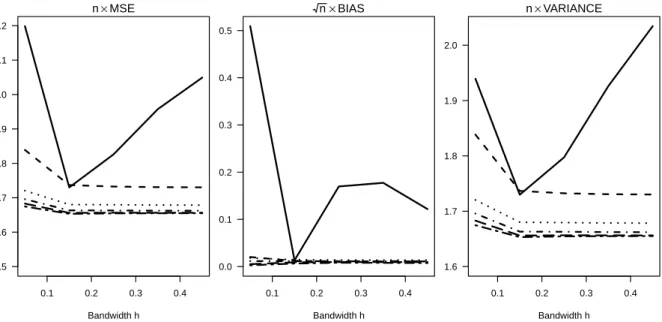
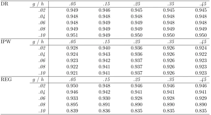
Fig-ure 1, we plot the Mean Squared Error (MSE), the bias, and the variance of the IPW estimator
as a function of the bandwidth h, and compare the results to those of the DR estimator for various values of the bandwidthg. In Figure 2, we plot the same three quantities for the REG estimator as a function of the bandwidth g, and compare the results to those for the DR esti-mator for various values of the bandwidth h. We also present the same results in table form in Table 1–3. One can clearly see that the bias of both IPW and REG varies substantially
with the respective bandwidth. To a lesser extend, this applies also to the variances of the two
estimators, especially in the case of IPW. As a consequence, the MSE shows strong dependence
on the bandwidth in both cases. It is minimized forh=.15 andg=.02, respectively, but these values would be very difficult to determine in an empirical application. For the DR estimators,
we observe that those using one of the two smallest bandwidths, i.e. either h=.05 or g=.02, exhibit somewhat different behavior from the remaining ones. For DR estimators usingh > .05 and g > .02, the MSE, bias and variance all exhibit only minimal variation with respect to the bandwidth. Their variance is substantially lower than that of IPW, and somewhat lower
than that of REG for larger values of g. It is also very close to the semiparametric efficiency bound, which is equal to about 1.644 in our simulation design. The DR estimators are also essentially unbiased for all bandwidth choices. DR estimators using either h =.05 or g =.02 have somewhat higher variance than those using larger bandwidths, but are also essentially
unbiased. As a consequence, they also compare favorably to both IPW and REG in terms of
MSE. In applications, we would recommend to implement DR estimators using bandwidths that
0.1 0.2 0.3 0.4 1.5 1.6 1.7 1.8 1.9 2.0 2.1 2.2
n×MSE
Bandwidth h
0.1 0.2 0.3 0.4 0.0 0.1 0.2 0.3 0.4 0.5
n×BIAS
Bandwidth h
0.1 0.2 0.3 0.4 1.6
1.7 1.8 1.9 2.0
n×VARIANCE
Bandwidth h
Figure 1: Simulation results: MSE, bias and variance of the IPW estimator for various values ofh(solid line), compared to results for the DR estimator with bandwidthgequal to .02 (dashed line), .04 (dotted line), .06 (dot-dashed line), .08 (long dashed line), and .10 (long dashed dotted line).
0.02 0.04 0.06 0.08 0.10 1.5
2.0 2.5 3.0
n×MSE
Bandwidth g
0.02 0.04 0.06 0.08 0.10 0.0 0.2 0.4 0.6 0.8 1.0 1.2
n×BIAS
Bandwidth g
0.02 0.04 0.06 0.08 0.10 1.60
1.65 1.70 1.75 1.80
n×VARIANCE
Bandwidth g
Figure 2: Simulation results: MSE, bias and variance of the REG estimator for various values ofg(solid line), compared to results for the DR estimator with bandwidthhequal to .05 (dashed line), .15 (dotted line), .25 (dot-dashed line), .35 (long dashed line), and .45 (long dashed dotted line).
are relatively large.
We also computed the empirical coverage probabilities of the confidence intervals CIj0.95
for j ∈ {DR, IP W, REG}, using again various bandwidths for estimating the nonparametric components. Results are reported in Table 4. Note that computing a confidence interval for
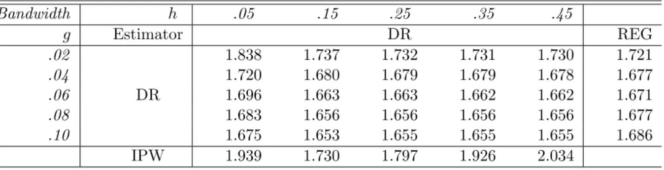
Table 1: Simulation Results: MSE of the IPW, REG and DR estimator for various bandwidth values (all results scaled by the sample size).
Bandwidth h .05 .15 .25 .35 .45
g Estimator DR REG
.02 1.839 1.737 1.733 1.731 1.730 1.725
.04 1.721 1.680 1.680 1.679 1.679 1.747
.06 DR 1.696 1.663 1.663 1.662 1.662 1.982
.08 1.683 1.656 1.657 1.656 1.656 2.497
.10 1.675 1.653 1.655 1.655 1.655 3.297
IPW 2.199 1.730 1.826 1.958 2.049
Table 2: Simulation Results: Bias of the IPW, REG and DR estimator for various bandwidth values (all results scaled by the square root of the sample size).
Bandwidth h .05 .15 .25 .35 .45
g Estimator DR REG
.02 0.020 0.012 0.011 0.011 0.011 0.065
.04 0.018 0.015 0.014 0.014 0.014 0.264
.06 DR 0.012 0.011 0.011 0.011 0.011 0.558
.08 0.005 0.009 0.010 0.010 0.009 0.906
.10 0.003 0.006 0.008 0.008 0.007 1.269
IPW 0.509 0.013 0.170 0.177 0.122
Table 3: Simulation Results: Variance of the IPW, REG and DR estimator for various bandwidth values (all results scaled by the sample size).
Bandwidth h .05 .15 .25 .35 .45
g Estimator DR REG
.02 1.838 1.737 1.732 1.731 1.730 1.721
.04 1.720 1.680 1.679 1.679 1.678 1.677
.06 DR 1.696 1.663 1.663 1.662 1.662 1.671
.08 1.683 1.656 1.656 1.656 1.656 1.677
.10 1.675 1.653 1.655 1.655 1.655 1.686
IPW 1.939 1.730 1.797 1.926 2.034
based on the REG estimator requires and estimate ofπo. Therefore all confidence intervals vary
with respect to both bandwidth parameters. Our results show that the coverage probability
of DR-based confidence intervals is extremely close to its nominal value for all combinations
of bandwidths we consider. IPW-based confidence intervals exhibit slight under-coverage for
small and large values ofhand good coverage properties for intermediate values, irrespective of the choice of g. REG-based confidence intervals have good coverage properties for g=.02 and
Table 4: Simulation Results: Empirical coverage probability of nominal 95% confidence intervals based on either the DR, IPW or REG estimator, for various bandwidth values.
DR g / h .05 .15 .25 .35 .45
.02 0.949 0.946 0.945 0.945 0.945
.04 0.948 0.948 0.948 0.948 0.948
.06 0.948 0.949 0.949 0.948 0.948
.08 0.949 0.949 0.949 0.949 0.949
.10 0.951 0.949 0.950 0.950 0.950
IPW g / h .05 .15 .25 .35 .45
.02 0.928 0.940 0.936 0.926 0.924
.04 0.924 0.943 0.936 0.926 0.922
.06 0.923 0.942 0.937 0.926 0.923
.08 0.922 0.941 0.937 0.926 0.923
.10 0.921 0.941 0.937 0.926 0.923
REG g / h .05 .15 .25 .35 .45
.02 0.950 0.948 0.946 0.946 0.946
.04 0.946 0.942 0.941 0.941 0.941
.06 0.933 0.930 0.928 0.928 0.929
.08 0.895 0.891 0.890 0.890 0.890
.10 0.839 0.836 0.835 0.835 0.835
6. Conclusions
Semiparametric two-step estimation based on a doubly robust moment condition is a highly
promising methodological approach in a wide range of empirically relevant models, including
many applications that involve missing data or the evaluation of treatment effects. Our results
suggest that SDREs have very favorable properties relative to other semiparametric estimators
that are currently widely used in such settings, such as e.g. Inverse Probability Weighting, and
should thus be of particular interest to practitioners in these areas. From a more theoretical
point of view, we have shown that SDREs are generally root-n-consistent and asymptotically normal under weaker conditions on the smoothness of the nuisance functions, or, equivalently,
on the accuracy of the first step nonparametric estimates, than those commonly used in the
literature on semiparametric estimation. As a consequence, the stochastic behavior of SDREs
can be better approximated by classical first-order asymptotics. We view these results as an
important contribution to a recent literature that aims at improving the accuracy of inference
A. Proofs of Main Results
A.1. Proof of Theorem 1. Statement (i) is immediately implied by statement (ii), and could also be
derived under weaker conditions. Statement (iii) follows from (ii) and a simple application of a Central
Limit Theorem. Statement (iv) follows from standard arguments, and we thus omit an extensive proof
for brevity. It thus remains to show statement (ii). To prove that result, note that it follows from the
differentiability ofψwith respect toθ and the definition ofθbthat
√
n(bθ−θo) = Γn(θ∗,p,bqb)−1√nΨn(θo,p,b bq)
for some intermediate value θ∗ between θ
o and θb, and Γn(θ, p, q) = ∂Ψn(θ, po, qo)/∂θ. It also follows from standard arguments that Γn(θ∗,bp,qb) = Γo+oP(1). Next, we consider an expansion of the term Ψn(θo,p,bqb). Using the notation that
ψp(Zi) =∂ψ(Zi, t, qo(Vi))/∂t|t=po(Ui),
ψpp(Zi) =∂2ψ(Zi, t, qo(Vi))/∂t|t=po(Ui),
ψq(Zi) =∂ψ(Zi, po(Ui), t)/∂t|t=qo(Vi),
ψqq(Zi) =∂2ψ(Zi, po(Ui), t)/∂t|t=qo(Vi),
ψpq(Zi) =∂2ψ(Zi, t1, t2)/∂t1∂t2|t1=po(Ui),t2=qo(Vi),
we find that by Assumption 4 we have that
Ψn(θo,p,bqb)−Ψn(θo, po, qo)
= 1 n
n
∑
i=1
ψp(Zi)(bp(Ui)−po(Ui)) + 1 n
n
∑
i=1
ψq(Zi)(qb(Vi)−qo(Vi))
+ 1 n
n
∑
i=1
ψppi (pb(Ui)−po(Ui))2+1
n
n
∑
i=1
ψiqq(qb(Vi)−qo(Vi))2
+ 1 n
n
∑
i=1
ψpq(Zi)(pb(Ui)−po(Ui))(qb(Ui)−qo(Ui))
+OP(∥bp−po∥3∞) +OP(∥qb−qo∥3∞).
By Lemma 2(i) and Assumption 5, the two “cubic” remainder terms are both of the orderoP(n−1/2). In Lemma 4–6 below, we show that the remaining five terms on the right hand side of the previous equation
are also all of the orderoP(n−1/2) under the conditions of the theorem. This completes our proof.
A.2. Proof of Theorem 2. Follows standard arguments from the literature on semiparametric
A.3. Proof of Theorem 3 and 4. These two results can be shown using the same arguments as for
the proof of Theorem 1. .
B. Axillary Results
In this section, we collect a number of auxillary results that are used to prove our main theorems. The
results in B.1 and B.2 are minor variations of existing ones and are mainly stated for completeness. The
result in B.3 is simple and stated seperately again mainly for convenience. Section B.4 contains a number
of important and original lemma that form the basis for our proof of Theorem 1.
B.1. Rates of Convergence of U-Statistics. For a real-valued functionϕn(x1, . . . , xk) and an i.i.d.
sample{Xi}ni=1 of size n > k, the term
Un=
(n−k)! n!
∑
s∈S(n,k)
ϕn(Xs1, . . . , Xsk)
is called akth order U-statistic with kernel functionϕn, where the summation is over the setS(n, k) of
alln!/(n−k)! permutations (s1, . . . , sk) of size kof the elements of the set {1,2, . . . , n}. Without loss
of generality, the kernel functionϕn can be assumed to be symmetric in itsk arguments, in which case
the U-statistic has the equivalent representation
Un =
(
n k
)−1 ∑
s∈C(n,k)
ϕn(Xs1, . . . , Xsk),
where the summation is over the setC(n, k) of all (nk)combinations (s1, . . . , sk) ofk of the elements of
the set{1,2, . . . , n}such thats1< . . . < sk. For a symmetric kernel functionϕn and 1≤c≤k, we also
define the quantities
ϕn,c(x1, . . . , xc) =E(ϕn(x1, . . . , xc, Xc+1, . . . , Xk) and
ρn,c= Var(ϕn,c(X1, . . . , Xc))1/2.
Ifρn,c= 0 forc≤c∗, we say that the kernel functionϕnisc∗th order degenerate. With this notation, we give the following result about the rate of convergence of akth order U-statistic with a kernel function
that potentially depends on the sample sizen.
kernel functionϕn, and that ρn,k <∞. Then
Un−E(Un) =OP
( k ∑
c=1
ρn,c
nc/2
)
.
In particular, if the kernelϕn isc∗th order degenerate, then
Un =OP
( k ∑
c=c∗+1
ρn,c
nc/2
)
.
Proof. The result follows from explicitly calculating the variance ofUn (see e.g. Van der Vaart, 1998),
and an application of Chebyscheff’s inequality.
B.2. Stochastic Expansion of the Local Polynomial Estimator. In this section, we state a
particular stochastic expansion of the local polynomial regression estimatorspbandqb, which is a minor
variation of results given in e.g. Masry (1996) or Kong et al. (2010). For simplicity, we state the result
only for the former of the two estimators, but it applies analogously to the latter by replacingpwith q
in the following at every occurrence. To state the expansion, we define the following quantities:
w(u) = (1, u1, ..., ul1p, u2, ..., ul2p, . . . , udp, ..., u
lp
dp)
T
wj(u) =w((Xp,j−u)/hp)·
Mp,n(u) = 1
n
n
∑
j̸=i
wj(u)wj(u)⊤Khp(Xp,j−u),
Np,n(u) =E(wj(u)wj(u)⊤Khp(Xp,j−u)),
ηp,n,j(u) =wj(u)wj(u)⊤Khp(Xp,j−u)−E(wj(u)wj(u) ⊤K
hp(Xp,j−u)).
To better understand this notation, note that for the simple case thatlp = 0, i.e. whenpbis the
Nadaraya-Watson estimator, we have that wj(u) = 1, that the term Mp,n(u) = n−1∑ni=1Khp(Xp,i−u) is the usual Rosenblatt-Parzen density estimator, thatNp,n(u) =E(Khp(Xp,i−u)) is its expectation, and that
ηp,n,i(u) =Khp(Xp,i−u)−E(Khp(Xp,i−u) is a mean zero stochastic term with variance of the order
O(h−dp
p ). Also note that with this notation we can write the estimatorbp(Ui) as
b
p(Ui) = 1 n−1
∑
j̸=i
where e1 denotes the (1 +lpdp)-vector whose first component is equal to one and whose remaining
components are equal to zero. We also introduce the following quantities:
Bn,p(Ui) =e⊤1Np,n(Ui)−1E(wj(u)Khp(Xp,j−Ui)(po(Xp,j)−po(Ui))|Ui) Sn,p(Ui) =
1 n
∑
j̸=i
e⊤1Np,n(Ui)−1wj(Ui)Khp(Xp,j−Ui)εp,j
Rn,p(Ui) = 1 n
∑
j̸=i
e⊤1
1
n
∑
j̸=i
ηp,n,j(Ui)
Np,n(Ui)−2wj(Ui)Khp(Xp,j−Ui)εp,j
We refer to these three terms as the bias, and the first- and second-order stochastic terms, respectively.
Here εp,j=Yp,j−po(Xp,j) is the nonparametric regression residual, which satisfiesE(εp,j|Xp,j) = 0 by
construction. With this notation, we obtain the following result.
Lemma 2. Under Assumptions 1–3, the following statements hold:
(i) For uneven lp≥1 the bias Bp,n satisfies
max
i∈{1,...,n}|Bp,n(Ui)|=OP(h
lp+1
p ),
and the first- and second-order stochastic terms satisfy
max
i∈{1,...,n}|Sp,n(Ui)|=OP((nh
dp
p /logn)−1/2)and max
i∈{1,...,n}|Rp,n(Ui)|=OP((nh
dp
p /logn)−1).
(ii) For anylp≥0, we have that
max
i∈{1,...,n}|pb(Ui)−po(Ui)−Bp,n(Ui)−Sp,n(Ui)−Rp,n(Ui)|=OP((nh
dp
p /logn)−3/2).
(iii) For∥ · ∥a matrix norm, we have that
max i∈{1,...,n}∥n
−1∑
j̸=i
ηp,n,j(Ui)∥=OP((nhpdp/logn)−1/2).
Proof. The proof follows from well-known arguments in e.g. Masry (1996) or Kong et al. (2010).
B.3. Functional Derivatives of DR moment conditions. In this section, we formally prove a
result about the functional derivatives of a DR moment conditions. Using the notation introduced in
the proof of Theorem 1, we obtain the following result.