www.geosci-instrum-method-data-syst.net/5/493/2016/ doi:10.5194/gi-5-493-2016
© Author(s) 2016. CC Attribution 3.0 License.
Auroral meridian scanning photometer calibration using Jupiter
Brian J. Jackel1, Craig Unick1, Fokke Creutzberg2, Greg Baker1, Eric Davis1, Eric F. Donovan1, Martin Connors3, Cody Wilson1, Jarrett Little1, M. Greffen1, and Neil McGuffin1
1Department of Physics and Astronomy, University of Calgary, Alberta, Canada
2Natural Resources Canada, Geological Survey, Geomagnetism Laboratory, Natural Resources Canada Geomagnetism Laboratory, Ottawa, Ontario, Canada
3Department of Physics and Astronomy, Athabasca University, Alberta, Canada
Correspondence to:Brian J. Jackel ([email protected])
Received: 4 March 2016 – Published in Geosci. Instrum. Method. Data Syst. Discuss.: 23 March 2016 Revised: 11 July 2016 – Accepted: 11 August 2016 – Published: 6 October 2016
Abstract.Observations of astronomical sources provide in-formation that can significantly enhance the utility of auro-ral data for scientific studies. This report presents results ob-tained by using Jupiter for field cross calibration of four mul-tispectral auroral meridian scanning photometers during the 2011–2015 Northern Hemisphere winters. Seasonal average optical field-of-view and local orientation estimates are ob-tained with uncertainties of 0.01 and 0.1◦, respectively. Es-timates of absolute sensitivity are repeatable to roughly 5 % from one month to the next, while the relative response be-tween different wavelength channels is stable to better than 1 %. Astronomical field calibrations and darkroom calibra-tion differences are on the order of 10 %. Atmospheric vari-ability is the primary source of uncertainty; this may be reduced with complementary data from co-located instru-ments.
1 Introduction
Interactions between the solar wind and the terrestrial mag-netic field produce a complex and dynamic geospace en-vironment. Ionospheric phenomena, such as the aurora, are connected to magnetospheric processes by mass and energy transport along magnetic field lines. Consequently, auroral observations provide information that can be used for remote sensing of distant plasma structure and dynamics. A single ground-based instrument can only view a small part of the global system, so a combination of instruments at different locations (e.g., Fig. 1 and Table 1) is required to span larger scales. Merging multiple data sets requires accurate
informa-tion about device characteristics such as timing, orientainforma-tion, and absolute spectral sensitivity.
Comprehensive calibration requires specialized equipment and skilled personnel that are typically available only at cen-trally located research facilities. With sufficient resources it is possible, at least in principle, to determine all device pa-rameters that are required to convert raw instrument data numbers to physically useful quantities. Practical limitations can result in random or systematic uncertainties which may impede quantitative scientific analysis. This is particularly relevant for large networks of nominally identical instru-ments, where ongoing calibration of each device may be ex-tremely challenging.
Even assuming ideal calibration at a central facility, many auroral instruments must be operated at remote field sites. Transfer between these locations requires a sequence of packing, shipping, and reassembly that is time-consuming, costly, and may unintentionally alter instrument response. Furthermore, intermittent calibration cannot distinguish be-tween a gradual drift or sudden changes.
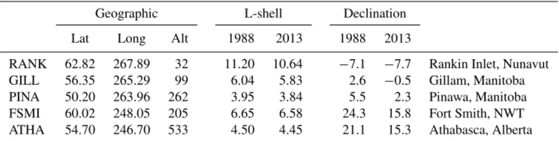
Table 1.Canadian meridian scanning photometer site information. Geographic latitude, longitude, and altitude are in degrees north, degrees
east, and meters above mean sea level (WGS-84). L-shell and magnetic declination from the IGRF model.
Geographic L-shell Declination
Lat Long Alt 1988 2013 1988 2013
RANK 62.82 267.89 32 11.20 10.64 −7.1 −7.7 Rankin Inlet, Nunavut
GILL 56.35 265.29 99 6.04 5.83 2.6 −0.5 Gillam, Manitoba
PINA 50.20 263.96 262 3.95 3.84 5.5 2.3 Pinawa, Manitoba
FSMI 60.02 248.05 205 6.65 6.58 24.3 15.8 Fort Smith, NWT
ATHA 54.70 246.70 533 4.50 4.45 21.1 15.3 Athabasca, Alberta
gill atha
fsmi
pina rank
50 60
70 80 Canada MSP locations
Figure 1. Canadian meridian scanning photometer site locations
(details in Table 1). Fan shapes indicate 4◦optical beam width for
altitudes of 110 and 220 km at elevations of 10◦above the horizon.
Dashed contours indicate magnetic dipole latitude (IGRF, 2015).
There is a long history of using astronomical sources to de-termine the alignment of auroral instruments (Stormer, 1915; Fuller, 1931; Chapman, 1934; Kinsey, 1963). Absolute cal-ibration using stellar spectra appears to be a more recent development (Gladstone et al., 2000; Whiter et al., 2010; Dahlgren et al., 2011; Wang, 2011; Wang et al., 2012; Grubbs et al., 2016). Detailed discussions of these topics are not al-ways provided in the primary scientific literature, but must often be extracted from conference proceedings, technical re-ports, and theses.
The focus of this paper is on the field calibration of a network of four auroral photometers using Jupiter as a stan-dard reference. Some key features of optical aurorae are pro-vided in Sect. 1.1, Sect. 1.2 introduces key calibration con-cepts and results, essential astronomical topics are presented in Sect. 1.3, and atmospheric effects are briefly reviewed in Sect. 1.4. An overview of instrument details is given in
Sect. 2, data analysis and results are in Sect. 3, discussion is in Sect. 4, followed by a summary and conclusions in Sect. 5.
1.1 Optical aurora
In regions of geospace where magnetic field lines can be traced to the Earth, some charged particles may travel down to altitudes where neutral densities are no longer negligible. Collisions with atmospheric atoms or molecules may transfer energy which can be re-emitted as photons. Spectral, spatial, and temporal features of the optical aurora contain informa-tion about geospace plasma properties, allowing for remote sensing of magnetospheric topology and dynamics.
Auroral spectra are dominated by several relatively bright lines and bands from atomic oxygen and molecular nitro-gen, with many other less intense features ranging from ex-treme ultraviolet through to far infrared. The intensity of au-roral emission at different wavelengths depends on precip-itation energy and atmospheric composition, as more ener-getic particles are able to penetrate to lower altitudes where constituents may be more or less abundant. Consequently, observations at multiple wavelengths can be combined to infer characteristics of the precipitating particles (Rees and Luckey, 1974; Strickland et al., 1989). These multispec-tral measurements can be challenging due to the wide dy-namic range between very bright 558 nm green-line (1– 100 kR) emissions and extremely faint 486 nm proton aurora (<100 R).
Meridian scan number
Elevation step number
Moon
Jupiter
Dawn Aurora
Stars
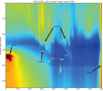
Figure 2.Keogram from meridian scanning photometer operating
at Gillam during the night of 20 December 2012 from 00:00 to dawn at 13:20 UT. Local midnight is approximately 06:00 UT (scan num-ber 720). Data counts have been clipped and logscaled in order to display Jupiter, stars, aurora, full moon, and dawn.
1.2 Instrument calibration
Optical designs can be modeled very precisely with mod-ern software tools, but instrument calibration provides es-sential information about the actual performance. System response is not necessarily constant, but can change either gradually (e.g., filter bandpass drift, decreased detector sensi-tivity) or abruptly (e.g., damage during shipping). Such prob-lems could be identified with calibration of instruments in the field. This process must be completely automatic, as many remote sites do not have full-time technical staff. It should be repeated frequently in order to identify abrupt changes in system response, but without interrupting or degrading nor-mal data acquisition. A regular schedule of measurements with portable low-brightness sources (LBSs) might satisfy some of these requirements, but would involve a substantial allocation of resources for repeated site visits.
In this report, we examine some of the strengths and lim-itations of astronomical calibration for auroral instruments. We focus on issues related to field cross calibration of MSPs which have been used extensively for auroral research (see Sect. 2 for details). However, many of these topics can also be applied more generally to other instruments used to study the optical aurora, such as all-sky imagers (ASIs).
A single ground-based instrument may measure photons with wavelengthsλarriving from angular locationsθ,φ. The distribution of incident lightI is convolved with the instru-ment response functionf to produce a measurementMwith errorMǫ:
M(θ, φ, λ)=f (θ, φ, λ)·I (θ′, φ′, λ′)+Mǫ(θ, φ, λ). (1)
For an ideal device,f would be a delta function andMwould be equal toI, but any real measurement will have limited res-olution. The goal of calibration or characterization is to de-termine the instrument response functionf in order to better understand the true source properties.
The general response function in Eq. (1) can be separated into a product of geometric sensitivityfGand spectral sensi-tivityfS:
fG(θ, φ)×fS(λ). (2) This approximation is not always valid (e.g., wide-angle op-tics coupled to a narrow-band interference filter) but can be usefully applied to many auroral instruments. For conve-nience, we introduce relative response functions (fˆ) that are normalized to a maximum of one, and combine all scaling into a single system constantC:
C× ˆfG(θ, φ)× ˆfS(λ). (3)
We show that using Jupiter for field calibration of MSPs pro-vides detailed knowledge aboutfˆG(θ,φ), estimates ofCthat
are comparable to darkroom calibration, and useful informa-tion about relative spectral responsefˆS(λ)at different wave-lengths.
1.2.1 Geometric
Calibration for auroral instruments with moderate (∼1◦) an-gular resolution can be achieved using point-like sources lo-cated sufficiently far from the entrance aperture. Angular re-sponse can be measured by either moving the source or ro-tating the instrument. The effective field-of-view (or beam shape) is often azimuthally symmetric around an optical axis with angular polar coordinatesθ0,φ0, in which case relative response can be expressed in terms of off-axis angleγ:
ˆ
fG(θ, φ)≈feG(γ;q1, . . ., qN) , (4)
and some set of instrument parameters qi (e.g., full-width half-max).
Ideally, each instrument would arrive at a field site in ex-actly the same condition as it left the darkroom. It would be operated exactly as intended (i.e., perfectly level and aligned north–south) without changes for the entire design lifetime. In practice, it may be difficult to achieve desired alignment to better than a few degrees. The initial orientation may subse-quently drift to some more stable state over months or years, with the possibility of more abrupt changes as the ground freezes in autumn and thaws in spring. In general, the rota-tion matrixRrequired to properly transform from device to local coordinates (e.g., azimuth and zenith angle) must be up-dated regularly in order to ensure that data are scientifically useful.
of the brightest stars. Accurate GNSS site location and mea-surement timing can be combined with astronomical cata-logs to predict the local orientation of each star. These can be converted into device coordinates and used to calculate observable quantities such as transit time and zenith angle. Discrepancies between predictions and observations can be minimized to determine optimal parameter values. A single night of good data may be sufficient to achieve subdegree accuracy, which is adequate for many auroral instruments.
Although stars are essentially point sources at infinity, other immutable properties (e.g., location, apparent motion, spectral radiance) may make them somewhat less tractable than darkroom calibration sources. Any given object will not always be visible in the night sky or pass through any specific location in an instrumental field of view. However, a substan-tial amount of useful information can be gathered over sev-eral days or months.
1.2.2 Spectral
The relative spectral response of an instrument is essential for quantitative multiwavelength analysis, such as estimat-ing precipitation energy (Rees and Luckey, 1974; Strickland et al., 1989). Spectral response can be most effectively deter-mined with a monochromatic source, such as
Z
dλ′fˆs(λ′)δ(λ−λ′)= ˆfs(λ′), (5) which can scan through the wavelength range of interest. For narrow-band devices it may be sufficient to observe a broad-band source S(λ) with known absolute spectral flux den-sity. If the source flux is roughly constant near some wave-lengthλjfor each device channel, as in
Z
dλfˆs(λ)S(λ)≈S (λk)
Z
dλfˆs(λ)=S (λk) 1λk, (6)
then the throughput for each channel may be expressed in terms of the effective bandwidth1λk.
Measurements of an absolutely calibrated LBS provide es-timates of the differential sensitivity to a continuum source characterized in terms of Rayleighs per nanometer. For dis-crete emission lines, the effective bandwidth is also required in order to determine the sensitivity to brightness as ex-pressed in Rayleighs. The equipment necessary for compre-hensive calibration (e.g., LBS and monochromator) is not always available at remote field sites, so different methods must be established. Many stellar sources provide spectra which are apparently broad band at typical auroral instru-ment resolutions on the order of 1 nm. Only relatively bright stars may be above the detection threshold, and absolute flux calibrated spectra are not available for all sources. Still, in certain cases it may be possible for astronomical calibration to produce accurate and repeatable estimates of differential sensitivity.
There does not appear to be a corresponding strategy to de-termine effective bandwidth in the field. Most stellar spectra are essentially constant in time, so individual sources cannot be used to determine a fixed instrument response. Combin-ing many different spectra might, in principle, allow us to distinguish between changes in effective bandwidth and to-tal sensitivity. However, this would require nearly simulta-neous observation of multiple absolutely calibrated sources with different spectral types. Low signal levels might also limit the accuracy of any estimates.
For this study, we proceed under the assumption that ab-solute spectral response cannot be independently determined in the field using only astronomical sources. We presume that normalized transmission integrated across each pass band,
Z
dλT (λ)ˆ ≡1λ T (λ)ˆ = [0,1], (7)
can be obtained in some other way, and acknowledge that si-multaneous changes across multiple channels may not be de-tected using methods considered here. For these reasons, we shall tend to focus on the differential calibration coefficientC˙ which can be determined using only astronomical methods. This quantity can also be directly compared to the results of darkroom calibration with an LBS. For auroral studies, data numbersDmust be converted to RayleighsR, and effective
bandwidth is required in order to calculateCR/D.
1.2.3 Radiometry
At a distance R from an isotropic point source with total power outputP0the irradiance (intensity)Swill be
S= P0
4π R2 W m
2, (8)
so that an observer at some distance r will intercept an amount of power,
Pδ=SAeff, (9)
proportional to the effective receiver surface areaAeff. Power from an extended source can be expressed in terms of a volume emission rateρ(r,θ,φ)integrated over the en-tire source region weighted by the receiver angular sensitivity G(θ,φ):
PV=
‹
dLG
4π 4π L≡ ∞
Z
0
drρ(r), (10)
where the radial integralLhas units of radiance (W m2sr1) and is often referred to as the “column emission rate”. For a uniform source radiance, the total received power
PV=
‹
dL(θ, φ)
depends on the product of the effective area and the effective solid angle. For any signal detected from some point source there will be an equivalent volume emission which would produce the same observed power. For a uniform emission region, the relationship
Pδ=PV→L= S
0 (12)
depends only on the effective solid angle.
Auroral intensity I is customarily expressed in units of
Rayleighs (Hunten et al., 1956; Baker, 1974; Baker and Romick, 1976; Brändström et al., 2012) which is related to photon radianceLγ via
4π Lγ(λ)≡I(λ) 1010photon s1m2 (13)
where the subscript E indicates energy flux andγ is photon number flux. For narrow-band channels
I(λ)=
Z
˙
I(λ)≈ ˙I1λ=4πS˙E 0
λ
hc1λ (14) converting differential radiant spectral density S˙ to equiva-lent Rayleighs per nanometer I˙ requires only the effective solid angle, which can also be estimated from observations of a point source. Working with Rayleighs requires some addi-tional knowledge in the form of the effective bandwidth1λ. As this is also true for darkroom LBS calibration, we focus here on relatingI˙ in Rayleighs per nanometer toS˙in watts per meter squared per nanometer.
1.3 Astronomical sources
Extraterrestrial objects have many properties which are re-quired for accurate calibration. Locations in the celestial sphere are known to arc-second resolution or better, which is sufficient for determining orientation and geometric re-sponse of most auroral instruments. Absolute spectral irra-diance profiles are available for many sources, providing op-portunities for radiometric calibration of narrow-band instru-ments. Total visible intensity of most sources is essentially constant, allowing for long-term monitoring of system per-formance. A single object can be viewed simultaneously by multiple instruments at nearby sites, facilitating quantitative intercomparisons.
Most astronomical objects are effectively point sources, and under good viewing conditions modern all-sky imagers can resolve hundreds of stars with a relatively short expo-sure time. Ironically, the presence of bright aurora or airglow can be a major source of error in radiometric calibration. For the MSP considered here, the total light from Vega passing through a 3 nm filter is approximately 200 Rayleighs, which is comparable to typical red-line airglow emissions. Even on a moonless night, continuum emissions can be on the order of 10 R nm−1, equivalent to stars of magnitude 2 as observed by our MSP. Note that there are only 50 stars of magnitude 2
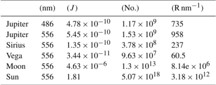
Table 2. Selected astronomical source irradiance at Earth.
En-ergy flux is joules per s m−2nm−1 and number flux is
pho-tons per s m−2nm−1 Rayleighs are for a viewing solid angle of
=0.002 steradians (2.9◦of arc).
(nm) (J ) (No.) (R nm−1)
Jupiter 486 4.78×10⁻¹⁰ 1.17×10⁹ 735
Jupiter 556 5.45×10⁻¹⁰ 1.53×10⁹ 958
Sirius 556 1.35×10⁻¹⁰ 3.78×10⁸ 237
Vega 556 3.44×10⁻¹¹ 9.63×10⁷ 60.5
Moon 556 4.63×10⁻⁶ 1.3×10¹³ 8.14e×106
Sun 556 1.81 5.07×10¹⁸ 3.18×10¹²
or brighter, and fewer than half of them are visible from the northern auroral zone at any given time.
Celestial source brightness spans a wide range and is usu-ally expressed in terms of logarithmic magnitudem: I=√5100m≈2.512m, (15) so that the relative intensity of two sources can be determined from the difference of their magnitudes. Absolute flux distri-butions as a function of wavelength are available for most of the brightest stars, including Vega (Colina et al., 1996), Sirius (Bohlin, 2014), and Arcturus (Blackwell et al., 1975; Griffin and Lynas-Gray, 1999). Other catalogs contain many other stars (Hayes, 1985; Alekseeva et al., 1996, 1997; Bohlin, 2007, 2014), but the majority may be too dim for reliable observation by typical auroral instruments.
Conversely, the sun is so bright that direct observation will saturate detectors designed for relatively faint aurora. Thuil-lier et al. (2003) provide an absolutely calibrated distribution of flux vs. wavelength at 1 AU with subnanometer spectral resolution. For a nominal instrument solid angle of 2 milli-steradians (3◦of arc) the apparent solar brightness at 556 nm is roughly 3 teraRayleighs per nanometer (Table 2). Daytime operations are only possible for systems that respond to an extremely narrow range of wavelengths (Galand et al., 2004). Although direct sunlight is unsuitable as a calibration source for most auroral instruments, scattering from other bodies in the solar system can provide more reasonable lev-els of brightness. The irradiance of an arbitrary bodyx can be modeled by isotropic emission from the sun incident on a sphere with radiusRx at distanceDSx, followed by
scatter-ing and absorption leadscatter-ing to some fraction of flux travelscatter-ing a distanceDxEto arrive at the top of Earth’s atmosphere. We group terms that depend on time and wavelength intoA(t ) andB(λ), respectively.
IxE(λ, t )=A(t )×B(λ) (16)
The wavelength-dependent termB(λ)contains irradiance in terms of the total solar irradiance (TSI∼1360 watts m−2) at a fixed distance of 1 AU, such as
500 1000wavelength [nm]1500 2000 0.0
0.5 1.0 1.5 2.0 2.5
Solar irradiance at Earth [W / m^2 / nm]
0.0 0.1 0.2 0.3 0.4 0.5 0.6
Jupiter albedo
500 550 600 650
Figure 3. Spectra of solar irradiance (green shaded curve) from
Thuillier et al. (2003) and Jupiter albedo (blue line) from Karkoschka (1998). Inset displays the same quantities for the range of wavelengths associated with most visible aurora.
where the solar powerPs(λ)and planetary albedoǫare both assumed to be time independent to 1 % or less.
The time-dependent termA(t )contains a phase correction factor8(ϕ)which accounts for any non-Lambertian scatter-ing as a function of angle ϕ between illumination and ob-server.
A(t )≡ R 2
xD2SE
DS2xDx2E8(ϕ)cos(φ) (18) For example, illumination from a full moon (φ=0) is re-duced by a factor of 3×10⁻⁶(m∼14) relative to direct sun-light. Despite this substantial decrease, the equivalent bright-ness of nearly 10 megaRayleighs per nanometer (Table 2) is still a hundred times brighter than the brightest aurora. For many instruments the angular size of the moon is nei-ther point-like nor beam-filling, requiring careful attention to details such as wavelength-dependent albedo varying across the disk (Kieffer and Stone, 2005), and making phase calcu-lations more complicated. For these reasons, the moon is not commonly used for calibrating auroral instruments.
After the moon, Jupiter is currently the brightest celestial object that can be regularly observed well past astronomical twilight. Peak visible magnitude is nearly 4 times that of Sir-ius (the brightest star), making Jupiter easy to identify in the night sky. A detailed spectral distribution of Jupiter’s albedo is given by Karkoschka (1998) (see Fig. 3). This can be com-bined with the solar spectrum of Thuillier et al. (2003) to predict the wavelength dependence of reflected light given in Table 3.
Other bodies in our solar system are less suitable as cal-ibration sources. Mercury is only visible from Earth during the daytime when looking near the sun. Venus can often be seen near dawn or dusk, but always with excessive amounts of indirect sunlight. Mars can be visible at night for several
1.5
2.0 2.5
3.0
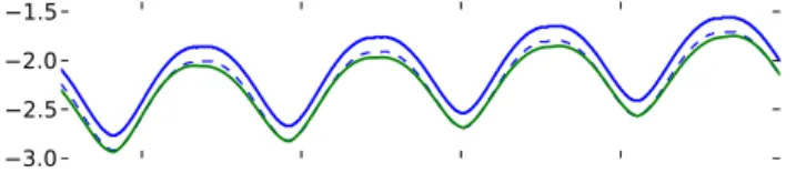
Figure 4.Jupiter as seen from northern auroral zone. Top panel:
ap-parent visual magnitude (negative is brighter). Different curves cor-respond to results from older references (V(1,0)= −9.25), newer references (−9.40), and calculations in this study (−9.426). Middle panel: declination, which is effectively the same for any terrestrial observer (parallax≈0). Bottom panel: relative air mass during tran-sit at Fort Smith, Gillam, Athabasca, and Pinawa.
months in a row, but this ideal configuration only occurs on alternate years. (Fig. 5). Albedo can vary considerably during dust storms and a wide range ofϕmeans that the phase func-tion8must be very precisely determined (Mallama, 2007). Saturn is roughly one-tenth as bright as Jupiter, with complex albedo variations due to ring geometry (V = −0.62 to+1.31) (Mallama, 2012).
The remaining outer planets are simply too dim for reliable detection by most auroral instruments.
As Jupiter and Earth each orbit around the sun, their rela-tive motion produces significant variations in apparent mag-nitude and position as shown in Fig. 4. In recent years Jupiter and the Earth have been closest during winter in Northern Hemisphere, maximizing brightness during the optimal pe-riod for observations with auroral instruments. As shown in Fig. 5, Jupiter transit at Gillam Manitoba currently occurs near sunrise in early October and sunset in February. An or-bital period of 11.89 years means that opposition will ad-vance by roughly 1 month per year. Optimal configurations with transit near midnight during northern winter started in 2011, will continue until 2016, and then begin again in 2022. Previous windows of opportunity include 1988– 1993 and 1999–2005. Any historical data acquired during these years could conceivably be retrospectively calibrated using Jupiter.
During this study, we identified a systematic difference be-tween our flux calculations for Jupiter and the correspond-ing magnitude value provided by widely available astronomy software (Downey, 2015) using the formula
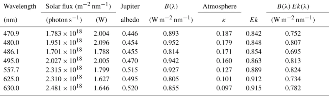
Table 3. Spectral variation of solar irradiance at Earth (Thuillier et al., 2003), albedo of Jupiter (Karkoschka, 1998), and atmospheric
extinction at Cerro Paranal (Patat et al., 2011). Column 5 is the product of solar irradiance at 1 AU and Jupiter albedo (defined asB(λ)in Eq.17) with units of watts per meter squared per nanometer. Atmospheric transmissionEk at zenith is related to extinctionκby Eq. (22).
Column 8 is the product of solar irradiance, Jupiter albedo, and atmospheric transmission with units of watts per meter squared per nanometer.
Wavelength Solar flux(m−2nm−1) Jupiter B(λ) Atmosphere B(λ) Ek(λ)
(nm) (photon s−1) (W) albedo (W m−2nm−1) κ Ek (W m−2nm−1)
470.9 1.783×10¹⁸ 2.004 0.446 0.893 0.187 0.842 0.752
480.0 1.951×10¹⁸ 2.096 0.454 0.952 0.179 0.848 0.807
486.1 1.701×10¹⁸ 1.788 0.455 0.814 0.171 0.854 0.695
495.0 2.027×10¹⁸ 2.005 0.470 0.942 0.160 0.863 0.813
557.7 2.315×10¹⁸ 1.799 0.515 0.927 0.127 0.889 0.824
625.0 2.310×10¹⁸ 1.627 0.495 0.805 0.101 0.912 0.734
630.0 2.481×10¹⁸ 1.646 0.520 0.855 0.097 0.915 0.782
Sidereal time [h]
Vega
Arcturus
Sirius Rigel Regulus
Mars Jupiter
Saturn
Transit at GILL 56.46 N 265.79 E from 01/01/2010–01/01/2016o o
Figure 5.Planetary right ascension over time indicated by thick colored lines (Mars is red, Saturn is blue, and Jupiter is green). Stars indicated
by thin black lines remain at constant RA. Sizes of small circles are proportional to lunar phase. Yellow shading indicates daytime extending to nautical twilight (sun 6◦below horizon).
where V(1, 0) is the magnitude at 1 AU with i=0 and 1m(φ)is the magnitude phase correction. Our results were calculated by entering standard distances into Eq. (18) with irradiance and reflection from Thuillier et al. (2003) and Karkoschka (1998). We obtained equivalent values of V(1, 0)≈ −9.426 that were nearly 20 % larger than the stan-dard result of V(1,0)= −9.25. Eventually, we discovered that the widely used lower value came from the 2nd edition of the Explanatory Supplement to the Astronomical Almanac (Seidelmann, 1992) but the most recent 3rd edition (Ta-ble 15.8, Seidelmann, 2005) now indicatesV(1, 0)= −9.40, which differs from our results by only 2 %. This exemplifies the degree to which we attempted to cross check our results against other references. It also demonstrates that even astro-nomical constants may be a work in progress.
1.4 Atmospheric effects
Light arriving at the top of the Earth’s atmosphere may un-dergo significant changes by the time it arrives at a ground-based observer. Gradients in the refractive index will bend ray paths, changing the apparent arrival angle. The magni-tude of this effect increases with zenith angle but is only on the order of 5 arcmin at 10◦elevation above the horizon. This might be important for astronomical applications, but is negligible for most optical auroral devices with precision requirements on the order of 1◦.
1m(λ, ζ )=κ(λ)X(ζ ), (20) whereκ(λ)is the extinction coefficient and the relative air massXas a function of zenith angleζ,
X(ζ )≈1+(1−c1) Z−c2Z2−c3Z3 Z=1−cosζ
cosζ , (21)
is equal to one at the zenith (i.e., X(0)=1) and increases by a factor of 5 at 10◦elevation above the horizon (Tomasi and Petkov, 2014). For convenience we may separate zenith angle and wavelength effects
E(λ, t )=Ek(λ)X(t ) Ek≡2.512−κ(λ) (22)
whereEk is the transmission through one standard air mass
(i.e., at zenith).
Empirical results from several nights of astronomical ob-servations near sea level (Vargas et al., 2002) show to-tal extinction ranging fromκ=0.312–0.604 andκ=0.180– 0.347 for standard blue and red filters, respectively. Zhang et al. (2013) foundκg=0.69 andκr=0.55 at a low-altitude
(170 m) high-humidity location. Tomasi and Petkov (2014) present an extensive review of optical air mass properties for the Arctic and Antarctic.
For this study, we use values from Patat et al. (2011) to provide a lower bound on extinction effects. The upper bound is estimated using an empirical model based on Vargas et al. (2002) and Zhang et al. (2013).
1.4.1 Transit zenith angle
Zenith angle at transit depends on the observer latitude 3 and declination of the source. Consequently, two observers viewing the same source from different latitudes will be look-ing through different air masses. This can produce systematic differences in brightness of a few percent or more depending on the latitude offset13and extinctionEk:
I2/I1∝E1Xk 1X≈ 1
cos(ζ1+13)− 1
cos(ζ1). (23) Calibration using Jupiter (or any other planet) will be fur-ther complicated by corrections for varying declination. Fig-ure 4 shows several years’ variation of air mass for Jupiter transit at the four field sites considered in this study. A sig-nificant transition occurs between large latitude-dependent extinction before 2011 to relatively uniform low levels after-ward. The consequences for this study are only on the order of a few percent, but are clearly evident in results presented in Sect. 3.3. This provides some assurance that our analysis procedures are accurate near the 1 % level. Of course, calcu-lating the effects of varying declination requires atmospheric extinction coefficients that may not be very well known. This is a challenge, but also an opportunity to test which extinc-tion models produce the best agreement with observaextinc-tions.
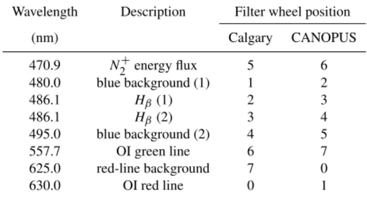
Table 4.MSP filter wheel sequence.
Wavelength Description Filter wheel position
(nm) Calgary CANOPUS
470.9 N2+energy flux 5 6
480.0 blue background (1) 1 2
486.1 Hβ (1) 2 3
486.1 Hβ (2) 3 4
495.0 blue background (2) 4 5
557.7 OI green line 6 7
625.0 red-line background 7 0
630.0 OI red line 0 1
Declination differences can even alter the intensity ratio between two different wavelengths (heterochromatic extinc-tion in Sterken and Manfroid, 1992),
I2/I1∝1EX(ζ )k 1Ek≡2.512κ(λ1)−κ(λ0), (24)
because extinction is a nonlinear function of air mass. This effect is considered in Sect. 3.4 and found to be significant.
2 Meridian scanning photometer
Auroral luminosity is often spatially anisotropic, with lati-tude structuring on scales of 1–100 km and longitudinal fea-tures extending from hundreds up to thousands of kilome-ters. Consequently, some instruments are designed with re-duced azimuthal coverage in exchange for improved sensitiv-ity along a latitude profile. These systems may be referred to as meridian imaging spectrographs (MISs) or meridian scan-ning photometers (MSPs) depending on the technology used for spectral discrimination and photon detection. In this pa-per, we explore issues related to field cross calibration of a specific MSP design that has been used extensively for au-roral research in Canada. Many of these topics can also be applied more generally to other auroral optical devices.
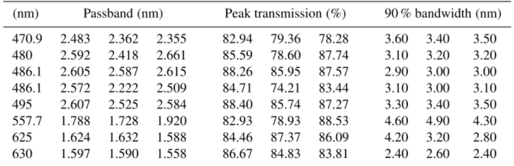
Table 5.Characteristics of three sets of nominally identical narrow-band filters. Passband is integral of transmission profile, 90 % bandwidth
is the range between 5 and 95 % points of the cumulative transmission.
(nm) Passband(nm) Peak transmission(%) 90 % bandwidth(nm)
470.9 2.483 2.362 2.355 82.94 79.36 78.28 3.60 3.40 3.50
480 2.592 2.418 2.661 85.59 78.60 87.74 3.10 3.20 3.20
486.1 2.605 2.587 2.615 88.26 85.95 87.57 2.90 3.00 3.00
486.1 2.572 2.222 2.509 84.71 74.21 83.44 3.10 3.00 3.10
495 2.607 2.525 2.584 88.40 85.74 87.27 3.30 3.40 3.50
557.7 1.788 1.728 1.920 82.93 78.93 88.53 4.60 4.90 4.30
625 1.624 1.632 1.588 84.46 87.37 86.09 4.20 3.20 2.80
630 1.597 1.590 1.558 86.67 84.83 83.81 2.40 2.60 2.40
Due to bandwidth limitations, most raw instrument output was downsampled by averaging in space and time in order to produce a uniform data stream for real-time transmission. Full high-resolution data were available over a serial cam-paign port. In later years, data loggers were used at some sites to record the full resolution data; several years of high-res MSP data are available for retrospective recalibration. The more extensive low-res data set is averaged into 17 latitude bins per scan, which is adequate for auroral science, but di-minishes the ability to resolve elevation from individual star transits.
The original CANOPUS MSPs were built by an indus-trial contractor (Johnston, 1989) based on a series of in-struments developed at the National Research Council of Canada (NRCC). Calibration of the prototype was carried out in 1985 by NRCC and the University of Saskatchewan, the results of which led to several design modifications. The first field system was commissioned at Gillam in Febru-ary 1986, with all four units operational by early 1988. By the late 1990s it was increasingly obvious that the instru-ments were nearing the end of their lifespan. The primary concern was the mirror motors which had driven several bil-lion steps, but many other issues (e.g., data acquisition, high voltage supplies, photomultiplier tubes) were also causing problems. Eventually, a lack of spare parts resulted in sig-nificant failures and data loss.
An MSP revitalization project was carried out at the Uni-versity of Calgary starting in 2007. The goal was to provide replacement systems with equivalent functionality. System design was based closely on the original instruments in order to minimize risk, with legacy mechanical and optical compo-nents reused where possible. Initial development was carried out on the legacy system at Rankin Inlet, which was bro-ken beyond repair. The detector was replaced with a new PMT, high-voltage supply, and pulse-counting circuit. Anti-reflection coatings were added to several optical elements, with system throughput optimized with predictions from op-tical modeling software and confirmed with quantitative test-ing. All of the old filters were replaced, as was the filter wheel motor. The scanning mirror assembly was upgraded to pro-vide 0.09◦ elevation steps (4000 steps per 360◦). Thermal
and power control systems were completely replaced. Low-level timing and synchronization is now coordinated by an FPGA, with a Linux PC-104 responsible for data acquisition and overall system control.
After darkroom calibration and local field trials, the new prototype system was deployed at Gillam and operated ad-jacent to the legacy system which was still functioning in-termittently. The original Gillam system was then upgraded and sent to Fort Smith (2009), the old Fort Smith sys-tem upgraded and installed at Pinawa (2010), and the old Pinawa system upgraded and moved to a new site near Athabasca (2011). Additional improvements were imple-mented in later systems, motivating a round of upgrades in 2012 to the Gillam and Fort Smith units. The entire re-build process took more than 4 years and involved multiple personnel at the University of Calgary. Despite careful atten-tion to tracking changes, there are still some funcatten-tional dif-ferences between the first and last refurbished systems. Many of these issues have been identified with internal calibration procedures, but astronomical sources provide useful insight about comparative instrument performance.
The new Calgary MSPs use the same filter wheel design as CANOPUS to acquire data from eight spectral channels, with 486.1 nm duplicated in order to increase SNR for faint proton aurora. Accurate radiometry of rapidly varying aurora requires effective simultaneous measurements of background and signal. This is accomplished by rotating the filter wheel at 1200 RPM (20 Hz) and gating the detector to provide suc-cessive 12.5 ms sample spacing. Some details about filter se-quencing is given in Table 4; for simplicity, all subsequent multichannel data will be ordered by increasing wavelength (blue to red).
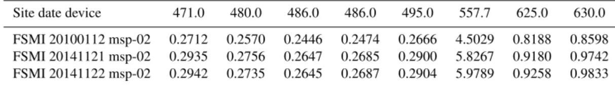
Table 6.Fort Smith MSP channel sensitivityC˙
R/D(Rayleighs/nanometer/count) determined by darkroom LBS calibration.
Site date device 471.0 480.0 486.0 486.0 495.0 557.7 625.0 630.0
FSMI 20100112 msp-02 0.2712 0.2570 0.2446 0.2474 0.2666 4.5029 0.8188 0.8598
FSMI 20141121 msp-02 0.2935 0.2756 0.2647 0.2685 0.2900 5.8267 0.9180 0.9742
FSMI 20141122 msp-02 0.2942 0.2735 0.2645 0.2687 0.2904 5.9789 0.9258 0.9833
1λj=
Z
dλTˆj(λ), (25)
is the relevant quantity for broad-band calibration sources, i.e., converting from Rayleighs per nanometer to Rayleighs. These data suggest typical passband and transmission varia-tions on the order of 5 % between different sets of filters.
Light which passes through the filters is detected by a photomultiplier tube (PMT) with photocathode quantum ef-ficiency ranging from 20 % at 400 nm to 2 % at 750 nm; this response was selected to maximize response for the faintHβ
emissions. A dynode chain amplifies each electron to pro-duce a cascade which triggers a pulse-counting circuit. The high-voltage power supply required for this process is quite stable over short intervals under ideal conditions, but may change during extended field operations. Photocathode ag-ing and high-voltage drift are likely to be the primary causes of any long-term reduction in system sensitivity.
The dead time of PMTs produces a nonlinear response at high count rates. This pulse pile-up effect can be largely re-moved if the time resolution τ of the system is known and is not significantly longer than the signal count interval. For the PMTs used in this study, nonlinearity only becomes im-portant for count rates greater than 105photons per second. These rates can be produced by very bright aurora but are not a problem for any astronomical sources except the sun and moon.
Meridian scans are achieved with a 45◦tilted mirror and a stepping motor. Many MSPs rotate the mirror at a fixed rate in order to produce data from evenly spaced elevations. Both the original and refurbished systems considered here instead utilize a sequence of variable steps chosen to produce nearly constant exposure times as a function of linear distance at auroral altitudes. This detail is relevant to this study because Jupiter transit profiles will be measured with different resolu-tion depending on transit elevaresolu-tion. The effects are expected to be small, but must be kept in mind when considering mul-tiyear variability.
2.1 System sensitivity
The relationship between incident photon flux P(λ) and measured channel count rateDk,
D=AeffMx1t
Z
dλP(λ)Tk(λ)Q(λ), (26)
depends on the effective aperture allowing photons into the system (Aeff), channel multiplexing efficiency (Mk), filter
transmission (Tk), measurement interval (1t), and the
detec-tor efficiencyQ(λ).
For wide-band input through narrow-band filters, the pro-cess can be written in terms of filter peak transmissionTkand
bandwidth1λk:
D(λi)≈P(λk) AeffMk1λkT (λk) 1t Q (λi) , (27)
from which we can isolate a coefficient of re-sponsekC#1/#2DP for each channel,
kC#1/#2DP =
D(λk)
P(λk)
=AeffMx1λkT (λk) 1t Q (λk) , (28)
in terms of measuredDand predictedPfor each filter
wave-length. In principle, this equation could be used to calculate coefficients in terms of fundamental properties of each in-strument. In practice, calibration coefficients are often esti-mated empirically by measuring sources with known bright-ness. For auroral applications the goal is to determine the differential sensitivity C#1/#2DR˙ relating data numbers to Rayleighs per nanometer.
2.2 Darkroom calibration
All systems have been calibrated at the University of Calgary using a low brightness source (LBS) with spectral radiance measured by the Canadian Institute for National Measure-ment Standards. Several sets of calibration results for one in-strument at different times are shown in Table 6. Results from two successive days (21 and 22 November 2014) agree to 1 % or better, suggesting that the calibration process is highly re-peatable. Earlier results from 2010 indicate that the system was about 5 % more sensitive in all channels, but with only two measurements over more than 4 years, it is impossible to determine whether this corresponds to a gradual decline or an abrupt change at some time during shipping or field operations.
3 Data analysis
There are five topics organized by which parameter is un-der consiun-deration and what supporting measurements are required. Results range from precise and absolute to un-certain and relative. Optical field of view is considered in Sect. 3.1, device orientation in Sect. 3.2, magnitude variation in Sect. 3.3, spectral ratios in Sect. 3.4, and absolute sensitiv-ity in Sect. 3.5.
Each of the MSPs considered in this study repeats a se-quence of scans from the northern to southern horizon. Ev-ery scan consists of multiple steps through a 160◦elevation range, with measurements acquired through multiple filters at each step. The resulting data stream has units of counts or simply data numbers (D) and can be represented by a [K,M, N] array of 16-bit numbers whereK=8 is the number of fil-ters,M=544 is the usual number of elevation steps for the rebuilt MSPs, and N=120 scans are acquired during each hour (30 s cadence).
Ephemeris software (Downey, 2015) was used to calcu-late the time and elevation corresponding to the transit of Jupiter through the local meridian containing the zenith and terminated by the celestial poles. To start, we assumed that instruments were perfectly level and had azimuths pointing directly north in order to obtain a starting point for identi-fying actual transits. A keogram subregion centered on the predicted transit was used to fit a two-dimensional general-ized Gaussian model:
D(x, y)=D0Exp
−
x √
2αx
βx
−
y √
2αy
βy
(29)
+B01+Bxx+Byy+Bxyxy ,
whereD0andB0are signal and background;y=y−y0and x=x−x0 are the elevation and time relative to the transit peak; x0,y0, andαx,y are profile widths; andβx,y are
scal-ing parameters. Jupiter transit profiles were initially modeled with a simpler bivariate Gaussian (βx=βy=2) which could
usually achieve model–data differences on the order of 10 %. The more general representation in Eq. (29) was introduced in an attempt to ensure that model error would not be a lim-iting factor for analysis at the 1 % level. We subsequently found that the coefficients also provided a useful measure for classifying transit quality, and more clearly identified minor azimuthal asymmetry in the optical response.
The polynomial background model is effective for mitigat-ing effects from dawn/dusk gradients and scattered moon-light. This significantly increases the number of transits which could be used for estimating orientation and field of view, although relatively few of these additional events are suitable for radiometric calibration. Figure 7 shows Gillam transit times obtained over several winter field seasons. Se-quences of good transits correspond to cloudless nights and gaps correspond to periods of poor visibility near full moon.
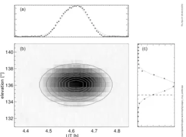
Figure 6. Gillam MSP observations of Jupiter on 22
Novem-ber 2011. Shading in central panel corresponds to counts for each scan and step (higher data numbers (DN) are darker, ranging from 0 to 1500 DN), contours indicate best 2-D Gaussian fit. Right panel is elevation profile obtained by averaging over time (symbols) and best fit Gaussian (dotted line). Top panel is time profile obtained by averaging over elevation. Dashed lines indicate the predicted transit time (off scale) and elevation for ideal north–south scan.
3.1 Field of view
Stars and distant planets are effectively point sources when viewed with a single pixel detector (PMT) through optics with angular resolution on the order of 1◦. Each MSP el-evation sweep over an astronomical source will produce a profile that corresponds to the vertical optical angular re-sponse. Similarly, a time sequence of observations from a fixed elevation should provide a complementary measure of horizontal optical beam shape. This is illustrated in Fig. 6 with a full two-dimensional (elevation and time) distribution of observed counts along with corresponding elevation and time profiles. Each profile is approximately Gaussian, and the combined two-dimensional pattern is fairly well modeled by the bivariate generalized Gaussian in Eq. (29). A complete transit profile extends over 10 min, during which time view-ing conditions may change considerably. In contrast, each el-evation sweep over Jupiter lasts for only a few seconds.
typ-Day of year
UT hour of day
Jupiter transit at Gillam 2010–2015
Quality Poor Fair Good
Figure 7.Jupiter transit time (UT) observed at Gillam during 2011–
2014 Northern Hemisphere winters. Each symbol corresponds to a single night; larger symbols indicate higher-quality transits.
0.9 1.0 1.1 1.2 1.3 1.4
Sidereal time width [ ] 0.9
1.0 1.1 1.2 1.3 1.4
Elevation width [ ]
Jupiter transit at Gillam 2010–2015
Quality Poor Fair Good
o
o
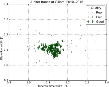
Figure 8.Optical beam width determined by fitting a generalized
Gaussian to observations of Jupiter by an MSP at Gillam over three winters.
ical beam solid angles are approximately 2.30×10⁻³ stera-dians with uncertainties of a few percent.
The effective solid angle0is essential for comparing flux from distant point sources to distributed auroral emissions. For several years of Fort Smith data, the average value was 2.07 msr with standard deviation of 0.12, and standard error of the mean was less than 1 %.
3.2 Orientation
An ideal MSP would be aligned to produce scans with pre-determined azimuth and elevation. For outdoor installations at remote field sites, it can be difficult to reduce leveling
er-2011 2012 2013 2014 2015 2016
Year 115
120 125 130 135 140 145 150 155
step angle [ ]
Jupiter transit at Gillam 2010–2015
o
Figure 9.Nominal stepping mirror elevation of Jupiter as observed
by Gillam MSP. Each symbol corresponds to one transit during a single night. Solid line indicates the actual elevation, while the dashed line is shifted by 7.5◦. Instrument alignment was quite good
before summer 2013, after which an unplanned tilt is evident.
rors below a few degrees. Geographic azimuth may be dif-ficult to precisely determine unless a detailed site survey is available. Alignment with magnetic north can also be chal-lenging unless the site is magnetically clean and there are no geomagnetic disturbances. Over longer periods the mag-netic declination may change significantly (see Table 1) due to secular variation in the geomagnetic field.
Fortunately, it is possible to accurately determine instru-ment orientation from transit observations. Starting with site locations obtained using GPS, observed transit times were used to calculate the actual elevation and azimuth of Jupiter for each night. These were interpreted in terms of two de-vice angles. First, azimuth offset was attributed to horizontal orientation of a level instrument. Second, the difference be-tween nominal mirror elevation and actual target elevation was attributed to instrument tilt from level.
Table 7.Instrument orientation and beam width from all good transits at Gillam and Fort Smith during each winter. Averages and standard
deviations in degrees for azimuth, tilt, beam width, and beam height. Solid angle average in millisteradians and percent standard error.
Site Year N Azimuth Tilt σh σv
GILL 2011–2012 73 6.65±0.16 0.52±0.32 1.04±0.07 1.12±0.06 2.224±1.5%
GILL 2012–2013 67 6.62±0.14 0.54±0.33 1.10±0.05 1.08±0.04 2.281±1.0%
GILL 2013–2014 46 4.81±9.25 6.52±0.77 1.10±0.07 1.09±0.06 2.301±1.8%
FSMI 2011–2012 64 10.35±0.16 0.59±0.29 1.06±0.07 1.11±0.05 2.257±1.4%
FSMI 2012–2013 57 10.00±0.26 0.87±0.19 1.12±0.10 1.07±0.06 2.282±2.0%
FSMI 2013–2014 54 10.50±0.24 0.66±0.22 1.12±0.09 1.06±0.04 2.274±1.6%
summertime operations. Fortunately, once the problem has been identified, it is relatively straightforward to make the necessary corrections to scientific data products.
A yearly summary of orientation parameters for two sites is presented in Table 7. For cases with 30 or more good tran-sits, the standard deviations are less than 0.5◦and uncertain-ties in the average (standard errors) are less than 0.1◦. This level of accuracy allows data to be accurately mapped into other coordinates (i.e., geographic); even minor changes to instrument alignment can be easily identified.
3.3 Magnitude variation
The signal intensity during each transit will depend on source brightness, instrument sensitivity, and atmospheric effects. This is complicated for Jupiter, as the apparent visual magni-tude varies due to changes in distance from Earth. Figure 10 illustrates the importance of this effect, with predicted varia-tion in apparent brightness following the upper bound of ob-servations. The lower set of events typically corresponds to apparent transit profile widths that are significantly different than the best-case values, and are likely due to non-ideal at-mospheric transmission (e.g., clouds or ice crystals). There are usually several dozen good transits per season; subse-quent analysis will focus on these events.
Effects due to variation in source brightness can be re-moved by normalizing all measured D cases to
magni-tudem=0:
D0=D×√5100mJ, (30)
where mJ is the apparent visual magnitude of Jupiter pre-dicted by the ephemeris. The resulting distribution of nor-malized magnitude at Gillam (not shown) has a fairly narrow peak with a sharp higher cutoff and a long tail of lower values corresponding to non-ideal viewing conditions. The 90th per-centile was found to be a simple and robust estimator of peak normalized brightness, while average and standard deviation are used to estimate uncertainty in seasonal averages. Results for Gillam and Fort Smith are presented in Table 8.
Normalized brightness for all Gillam transits over 3 years is shown in Fig. 11. Linear fits to the data give a slight pos-itive slope of roughly 2 % per year, but with statistical
un-Figure 10.Peak counts from Jupiter at Gillam over three winters.
Large symbols are transits with narrow widths, small symbols are noisier profiles. Solid line is variation in apparent visual magnitude of Jupiter, dashed line indicates the change in extinction due to dou-bling air mass (1κ=0.15).
certainty that includes zero. This is consistent with a stable system response at blue wavelengths, although variations on the order of 5 % cannot be excluded.
If the linear trend were significant, this would mean the instrument was becoming slightly more sensitive over time, which seems unlikely. Closer examination of the data found that most of the variation is due to a 5 % jump between 2012 and 2013 after which the signal levels remain essentially con-stant. The jump did not correspond to any system mainte-nance or modifications. A nearly identical pattern was ob-served at Fort Smith, further suggesting that the underlying cause was not instrumental.
Table 8.Magnitude normalized intensity and self-normalized spectral sensitivity for Gillam and Fort Smith. Column 3 is the number of
good transits available from each winter season. Column 4 is the 90th percentile of intensity. Column 4 is the source-normalized brightness (Eq. 30). Remaining columns are channel brightness normalized to average of two 486 nm observations.
Site Year N 90 % D0 471 480 486 486 495 558 625 630
GILL 2011–2012 73 530.3 425±143 0.914 1.054 0.997 1.003 1.052 0.087 0.415 0.382
GILL 2012–2013 67 572.7 474±133 0.927 1.033 1.007 0.993 1.073 0.087 0.399 0.359
GILL 2013–2014 46 582.6 487±141 0.914 1.042 0.997 1.003 1.061 0.018 0.376 0.366
FSMI 2011–2012 64 844.9 651±224 0.915 1.063 1.000 1.000 1.055 0.071 0.395 0.379
FSMI 2012–2013 57 873.2 732±199 0.933 1.043 1.009 0.991 1.066 0.102 0.400 0.341
FSMI 2013–2014 54 877.0 715±228 0.907 1.056 1.003 0.997 1.049 0.053 0.387 0.347
Figure 11.Gillam transit events from Fig. 10 normalized to
magni-tude 0 using Eq. (30).
in declination corresponds to transmission differences of 74.9 vs. 80.4 %. Adding this correction to normalized bright-ness reduces the linear trend to zero, although with consider-able uncertainty.
3.4 Spectral ratio
Absolute radiometric calibration with Jupiter is complicated by variability in observed brightness, and absolute spectral sensitivity is similarly challenging. Working with relative spectral response removes changes in source brightness, al-lowing us to focus on instrumental and atmospheric effects. In order to reduce statistical uncertainty, we have normalized all channels to the average of the twinHβ channels. Results
are summarized in Table 8.
Factoring out external brightness variation provides useful information about internal stability of different wavelength channels. Averages for normalized blue channels are essen-tially constant to within 1 % year to year. This result provides some reassurance about relative filter stability, but cannot exclude the possibility of any change which might produce
Figure 12.Ratio of 630.0 nm to average of two 486.1 nm channels
vs. time. Large symbols correspond to good transits and small sym-bols to noisier events.
identical changes in all channels (e.g., high-voltage supply drift, optical defocusing).
Red channels exhibit more variability on both shorter and longer timescales as shown in Fig. 12. One notable feature is a clear drop after the first season, followed by 2 years of rel-ative stability. This might be attributed to some wavelength-dependent change in sensitivity such as photocathode aging or filter delamination. However, exactly the same pattern is observed at all four sites, suggesting a cause that is external rather than instrumental.
Table 9.Calibration coefficientC#1/#2P Destimated at Gillam using a single transit on 11 November 2011. Atmospheric effects are neglected.
486.1 (nm) Channel wavelength
1501 (DN) Peak data number
5.191×10¹⁷ (photon)/(m2s−1nm−1) Solar photon flux at 1 AU
5.328×10⁻¹⁰ Geometric factorA(t )
0.455 Jupiter albedo
1.061×10⁹ (photon)/(m2s−1nm−1) Jupiter photon flux at Earth
7.067×10⁵ (photon)/(m2s−1nm−1D) Calibration coefficientC#1/#2P D
0.799 Extinction atζ=45.6◦
logI1/I2+log(2.512)−x (κ1−κ2)=logD1/D2, (31) gives a slope ofκred−κblue≈0.38, which is generally con-sistent with other results considered in Sect. 1.4. Since this estimate is produced by combining a large number of transits obtained during a wide range of atmospheric conditions, we do not place too much weight on the precise value. The im-portant result is that spurious trends in wavelength ratios can be modeled well enough to allow detection of real changes on the order of 5 %.
3.5 Absolute sensitivity
System sensitivity defined in Eq. (28) provides a measure of the data count rate D produced by one Rayleigh per
nanometer R˙ of extended luminosity. This can be related to the differential irradiance of an ideal point source using Eq. (14). Losses due to atmospheric effects can be modeled with Eq. (20). The combination of these three equations,
C#1/#2DR˙=1010D
˙ Sγ
0 4π2.512
+κX, (32)
gives an expression for calibration coefficients in terms of five physical quantities (see also p. 42 of Wang, 2011). Three of these terms are easily estimated, while the other two present some challenges.
The differential number fluxS˙γ of solar photons scattered
from Jupiter and arriving at the top of the Earth’s atmo-sphere is only subject to uncertainties in the solar spectrum and Jupiter’s albedo, both of which are known to 1 % or bet-ter. The effective air massX(ζ (t ))depends on the apparent zenith angle which can be calculated for any arbitrary time. The effective solid angleis either known a priori or can be estimated from transit profiles; from Sect. 3.1 the uncertainty of an unbiased estimate will be less than 1 %, but systematic bias on the order of 5 % is also a possibility.
The extinction coefficient spectrum κ(λ) can be highly variable, can have a major effect on received signal levels, and cannot be accurately estimated from the MSP data. In the absence of other information, the best we can do is identify
an upper envelope containing the brightest events and assume that they correspond to the minimum possible extinction val-ues. This approach seems to produce intrinsic variability less than 5 %, but does not address the issue of systematic bias.
Each transit could potentially provide a measured value for D. A simple calculation of Poisson uncertainty for the
entire profile would be on the order of 1 % assuming good transits with peaks in excess of 2000 counts. This result may be overly optimistic given the complicated nature of many transits. An alternative approach is to examine sequences of transit profiles, focus on clusters of bright events in the top quartile or decile, and assume that they provide an overmate of the intrinsic variability. This approach produces esti-mated uncertainties ranging from 1 to 5 %.
Data from a single transit can be scaled by model flux den-sity from Eq. (18) to obtain an empirical estimate of the sys-tem calibration coefficientC. An example is provided in
Ta-ble 9 for the 22 November 2011 transit at Gillam using the pair of nominally identical 486 nm channels as an example. Fitting a two-dimensional Gaussian model to each channel separately produced very similar peak values: 1501.14 and 1501.54 DN. Appropriate model values from Table 3 can be used to predict input photon flux (neglecting atmospheric ef-fects) and estimate a system calibration coefficient relating flux from a point source to measured data numbers.
Calculation up to this point has consisted of multiplying several quantities, each with relative uncertainty of a few percent or less. These errors are negligible in comparison to atmospheric variability. The 486.1 nm extinction factor at zenith could vary between 0.73 and 0.84 for fair to good visi-bility, and 0.64–0.78 atζ=45◦. Lower elevations and worse viewing conditions will further attenuate incoming flux. Ne-glecting extinction will provide a lower bound for empirical sensitivity, as reduced flux requires higher sensitivity in order to produce the same observations.
Table 10.Sensitivity for each channel in data numbers (counts) per Rayleigh per nanometerC#1/#2DR. Asterisks for Gillam 2012 green line correspond to a calibration without the standard neutral density filter.
Year N 471 480 486 486 495 558 623 630
GILL 2011 59 0.2478 0.1816 0.2507 0.2427 0.2002 1.6296 1.0857 0.9721
GILL 2012 60 0.2114 0.1603 0.1698 0.1702 0.1718 – 0.8244 0.8764
GILL 2013 39 0.1434 0.1280 0.1169 0.1174 0.1365 1.3462 0.5802 0.5037
FSMI 2011 51 0.0734 0.0707 0.0615 0.0611 0.0704 1.5203 0.3267 0.3525
FSMI 2012 47 0.1239 0.1182 0.1096 0.1113 0.1292 3.6000 0.6915 0.6828
FSMI 2013 52 0.1316 0.1222 0.1164 0.1164 0.1307 3.3278 0.5578 0.3469
Figure 13.Total counts in four blue channels (excluding 470.9 nm)
as a function of predicted photon flux density. The small “+” signs indicate all cases, medium “x” signs indicate good beam widths, and large squares indicate nearness to robust fit line. Flux model includes solar spectrum, illumination geometry, Jupiter albedo, and terrestrial atmospheric extinction as in Table 3.
(Sect. 3.1). Most points cluster near a common linear trend, but there are also quite a few low-brightness outliers. A ro-bust (least absolute deviation) linear model provides a plau-sible fit that is insensitive to outliers. Points within a gener-ous range around the robust fit are classified as high quality and used for subsequent analysis, including standard least squares estimates of intercept and slope CD/P. Figure 13
shows classification and fitting results for the combined blue channel data. This automated process produces reasonable results for all the data considered in this study. Channel cali-bration coefficients for Gilliam and Fort Smith are presented in Table 10, and Fort Smith results plotted in Fig. 14. More sophisticated algorithms for further studies could explicitly include the asymmetric nature of extinction, i.e., hard upper bound on theoretical maximum.
2010 2011 2012 2013 2014 2015
Year 2.5
3.0 3.5 4.0 4.5 5.0
Sensitivity [counts per Rayleigh]
Darkroom Airless Best case
Figure 14.Sensitivity for the FSMI MSP 486.1 nm channels. Green
circles are values obtained during darkroom calibration in 2010 and 2014; nominal linear trend of−2 % yr−1indicated by dashed
line. Blue symbols are values obtained by averaging three best val-ues over 10-day intervals and standard deviation indicated with er-ror bars;xvalues are without any atmospheric correction; squares are with clear sky model.
4 Discussion
When auroral instruments operate unattended for long peri-ods of time at remote locations, frequent comprehensive on-site calibration may not be feasible. If celestial objects can be identified in standard data streams then these may serve as the basis for alternative independent calibration procedures.
Jupiter’s peak intensity is greater than the brightest star, but less than the moon, so there is no risk of saturating most auroral detectors. It is effectively point-like, has a predictable trajectory, and absolute spectral flux can be calculated from existing albedo and solar irradiance measurements. Unlike stars, planets are not fixed in celestial coordinates, mean-ing that transit altitude is not constant. This minor compli-cation actually provides an opportunity to study the effects of changing zenith angle on atmospheric extinction.
4.1 Atmospheric effects
Atmospheric transmission is likely to be the largest source of uncertainty for high SNR applications. Reducing this uncer-tainty will require estimation of extinction coefficients that are appropriate for each transit. Our preliminary attempts to determine these parameters using multispectral MSP data were not successful, but this problem may yield to more so-phisticated analysis. In principle, extinction coefficients can be found simply by measuring the apparent magnitude of a single star at a given wavelength over a range of different zenith angles. Improved precision can be achieved by com-bining data from multiple stars. Many auroral observatories include all-sky camera systems which can image dozens or hundreds of stars. However, the optical response (flat field) of these systems is also a strong function of axial angle, which for an ASI is usually directed towards the zenith. Accurate flat fields will be essential for accurate extinction estimates. Recent work by Duriscoe et al. (2007), Olmo et al. (2008), and Román et al. (2012) might be adapted for auroral appli-cations.
It is tempting to avoid the complexity of atmospheric vari-ation by using only a small number of good days to deter-mine calibration parameters. One obvious limitation of this approach is that it cannot reliably detect short term changes in instrument response. More importantly, all auroral obser-vations are subject to exactly the same atmospheric issues. A constant emission feature moving from the horizon to zenith will appear brighter even after accounting for viewing ge-ometry (i.e., van Rhijn correction) simply due to the reduc-tion in total air mass between auroral altitudes and a ground-based observer. Atmospheric effects may be negligible when looking directly upward through clear skies, but critically im-portant at low elevations and non-ideal viewing conditions. These effects would be even more pronounced at shorter wavelengths (e.g., 427.8 and 391.4 nm) often used in auro-ral studies.
4.2 Retrospective calibration
Some auroral instruments only acquire data during short-term campaigns, but many are operated in support of longer-term science objectives. Not all devices are fully calibrated before being deployed and few are calibrated on a regular ba-sis. Even when the resulting data overlap in space and time,
quantitative comparison may not be possible. Astronomical observations of bright sources such as Jupiter can provide a basis for retrospective cross calibration of historical data sets. The original CANOPUS meridian scanning photome-ter array (MPA) is a good example. Digital low-resolution binned data are available starting in early 1988 and continu-ing until sprcontinu-ing 2005. Some higher-resolution data are avail-able for the transition period from 2005 to 2010, after which all refurbished instruments were operating in the same high-resolution mode. The 16 years of low-res data alone extend well beyond one solar cycle and could span more than two if merged with newer data.
However, certain kinds of quantitative analysis are limited by the lack of radiometric calibration. Some key parameters (e.g., filter bandwidth and channel sensitivity) were deter-mined for each system, but the supporting documentation is very limited. Mechanical and electrical subsystems were reg-ularly maintained and repaired, but there was no correspond-ing recalibration schedule. Some terminal calibration proce-dures were carried out during the 2005–2010 transition, but by this point the instruments were often not functioning re-liably. In order to confidently identify long-term geophysical trends in these data, it is essential to have some sense of how instrument performance changed over the same timescales.
A preliminary survey of the CANOPUS MPA data archive has confirmed the feasibility of astronomical calibration and also identified some significant challenges. First, only the brightest few stars are visible even with optimal viewing con-ditions. Jupiter can be clearly identified, but at count rates much lower than obtained by the newer systems, and con-sequently with much greater uncertainty. Elevation steps are combined into 17 latitude bins which effectively removes the ability to determine instrument tilt. More generally, it elimi-nates virtually all information about the optical beam shape in that direction, including that required to confidently esti-mate the effective solid angle0. Finally, the decreased scan cadence of one per minute will slightly reduce the accuracy of azimuth estimates. Despite these limitations it should still be possible to estimate absolute sensitivity using Jupiter tran-sits during extended intervals at both ends of the project: 1989–1993 and 1999–2005. Other bright stars or planets might be used to fill in the intervening period.
5 Conclusions