www.ann-geophys.net/33/185/2015/ doi:10.5194/angeo-33-185-2015
© Author(s) 2015. CC Attribution 3.0 License.
Tidal signatures of the thermospheric mass density and zonal wind
at midlatitude: CHAMP and GRACE observations
C. Xiong1,2, Y.-L. Zhou2, H. Lühr1,2, and S.-Y. Ma2
1Helmholtz Centre Potsdam, GFZ German Research Centre for Geosciences, Telegrafenberg, 14473 Potsdam, Germany 2Department of Space Physics, College of Electronic Information, Wuhan University, 430079 Wuhan, China
Correspondence to:C. Xiong ([email protected])
Received: 22 September 2014 – Revised: 7 January 2015 – Accepted: 7 January 2015 – Published: 4 February 2015
Abstract. By using the accelerometer measurements from CHAMP and GRACE satellites, the tidal signatures of the thermospheric mass density and zonal wind at midlatitudes have been analyzed in this study. The results show that the mass density and zonal wind at southern midlatitudes are dominated by a longitudinal wave-1 pattern. The most promi-nent tidal compopromi-nents in mass density and zonal wind are the diurnal tides D0 and DW2 and the semidiurnal tides SW1 and SW3. This is consistent with the tidal signatures in the F re-gion electron density at midlatitudes as reported by Xiong and Lühr (2014). These same tidal components are observed both in the thermospheric and ionospheric quantities, sporting a mechanism that the non-migrating tides in the up-per atmosphere are excited in situ by ion–neutral interactions at midlatitudes, consistent with the modeling results of Jones Jr. et al. (2013). We regard the thermospheric dynamics as the main driver for the electron density tidal structures. An exam-ple is the in-phase variation of D0 between electron density and mass density in both hemispheres. Further research in-cluding coupled atmospheric models is probably needed for explaining the similarities and differences between thermo-spheric and ionothermo-spheric tidal signals at midlatitudes. Keywords. Ionosphere (ionosphere–atmosphere interac-tions; mid-latitude ionosphere; wave propagation)
1 Introduction
The ionosphere–thermosphere (IT) system represents the transition region from Earth’s atmosphere to space. Under-standing ionosphere–thermosphere dynamics and electrody-namics is paramount when considering the necessity for more accurate space weather forecasts. In recent years, both
observational and theoretical studies have shown that a larger part of the variability in the global IT system is associated with lower atmospheric processes, especially the influence of various waves. These waves behave as global-scale oscilla-tions in temperature, wind, and density with periods that are harmonics of a solar day and are referred to as atmospheric “migrating” and “non-migrating” tides (e.g., Chapman and Lindzen, 1970; Forbes, 1995). Migrating tides propagate westward with the apparent motion of the sun; therefore, they are sun-synchronous and longitude independent when observed at constant local time. They are prompted primarily by the absorption of solar energy by tropospheric water and water vapor, as well as stratospheric ozone (Oberheide et al., 2002). Non-migrating tides are excited for instance by zonal asymmetries (e.g., topography, land-sea differences, longi-tude dependence of absorbing species) (Forbes et al., 2003) or by nonlinear interactions between the migrating diurnal tide and planetary waves (Hagan and Roble, 2001) or grav-ity waves (McLandress and Ward, 1994). Another important source for non-migrating tides is the latent heat release in the troposphere (Hagan and Forbes, 2002).
In general, these atmospheric tides in the universal time (UT) frame can be expressed as
An,scos(nt+sλ−φn,s), (1)
whereAn,s is the amplitude,n denotes the harmonic of a
solar day, is the rotation rate of the Earth, t is the uni-versal time,s is the zonal wavenumber,λis the longitude, andφn,s is the phase of the tides (Forbes et al., 2006). In this
lo-cal time (LT) every 11 and 13.5 days, respectively, thus tak-ing their daily measurements at a quasi-constant local time. When converting the tidal description from UT to LT using
t=tLT−λ/ , Eq. (1) can be expressed as
An,scos(ntLT+(s−n)λ−φn,s). (2)
For migrating tides (s=n), the amplitude are longitude in-dependent (s−n=0) in the local time frame. While non-migrating tides (s6=n) will present longitudinal patterns at wavenumbers |s−n|. In accordance with previous defini-tions, throughout this study we will use the notation DWs and DEs for labeling the tidal components. The first letters D, S, and T stand for diurnal, semidiurnal, and terdiurnal; the second letters E and W, for eastward or westward propagat-ing; and the final number quantifies the azimuthal wavenum-ber. D0 represents a wave that is increasing and decreasing simultaneously at all longitudes with a diurnal period. Sta-tionary planetary waves are labeled as SPWs and the number at the end quantifies the number of maxima around the globe. The phase of the tides defines the time when the wave crest passes the 0◦longitude meridian, while in the case of SPWs, the longitude of the wave maximum is given.
Due to the rapid development of the upper atmospheric observations in the past decade, significant progress has been made in the investigation of the coupling of the up-per atmosphere and ionosphere. At equatorial and low lat-itude regions, the longitudinal wavenumber-4 (WN4) and wavenumber-3 (WN3) patterns have been widely studied, based on model simulations and observations from sun-synchronous and slowly precessing platforms in space (e.g., Sagawa et al., 2005; Immel et al., 2006; England et al., 2006, 2010; Forbes et al., 2006; Lühr et al., 2008, 2012; Ober-heide et al., 2009, 2011b; Liu et al., 2009; Häusler and Lühr, 2009). These WN4/WN3 patterns are considered to be as-sociated with the eastward-propagating non-migrating tides DE3/DE2, that are primary excited by latent heat release in the tropical troposphere (Hagan and Forbes, 2003; Immel et al., 2006; Wan et al., 2010). Hagan et al. (2009) reported the existence of stationary planetary wave-4 (SPW4) oscillation in the upper mesosphere and lower thermosphere (MLT) re-gion, caused by the nonlinear interaction between DE3 and the migrating tide DW1. Since then, the importance of sta-tionary planetary waves, SPW4/SPW3, contributing to the longitudinal WN4/WN3 patterns in the upper atmosphere, has also been supported by both model simulations (e.g., Oberheide et al., 2011a; Pancheva et al., 2012) and in situ observations (e.g., Kil et al., 2010; Lühr and Manoj, 2013; Xiong and Lühr, 2013; Chang et al., 2013).
At midlatitudes, in our recent work Xiong and Lühr (2014), we have reported prominent longitudinal wave-1 and wave-2 patterns in electron density of the southern and northern midlatitude summer nighttime anomaly (MSNA) features, respectively. The MSNA refers to the phenomena of nighttime electron density anomalous enhancements at midlatitudes during local summer seasons. In the Southern
Hemisphere, the MSNA (also named Weddell Sea anomaly – WSA) was first observed by ground-based ionosondes in the 1950s (e.g., Bellchambers and Piggott, 1958; Penndorf, 1965) and further detailed by using satellite observations in recent years (Burns et al., 2008; Lin et al., 2009; He et al., 2009). The northern WSA-like features (with two elec-tron density anomalous regions) have later been widely in-vestigated by various observations (Lin et al., 2009, 2010; Thampi et al., 2009; Liu et al., 2010). The generation of the MSNA is still an open issue, and several potential mech-anisms have been proposed that try to explain the phe-nomenon. The wind mechanism is consistent with most of the observations, which can be interpreted as a combined re-sult of thermospheric wind, solar photo-ionization, and the local magnetic field configuration (Rishbeth, 1967, 1968; Dudeney and Piggott, 1978; He et al., 2009). Other mech-anisms such as the transportation of plasma from the dayside ionosphere and the downward flux from the plasmasphere have also been proposed (Burns et al., 2008). By employing a three-dimensional physics-based ionosphere model, SAMI3 (Sami3 is Also a Model of the Ionosphere), coupled with the Thermosphere–Ionosphere Electrodynamics General Circu-lation Model (TIE-GCM) and the Global Scale Wave Model, Chen et al. (2013) reported a clear eastward movement of the southern MSNA (see their Fig. 2b). They further ex-plained that the standing diurnal tide (D0) dominates the ver-tical neutral wind causing the southern MSNA feature, and the tide manifests itself as a diurnal eastward-propagating wave-1 pattern. Our recent study confirmed the eastward movement of the MSNA in both hemispheres from in situ measurements of the CHAMP and GRACE missions (Xiong and Lühr, 2014). From the tidal perspective, the prominent MSNA features have further been interpreted as the simulta-neous constructive interferences of the tidal components D0, DW2, and stationary planetary wave SPW1 in the Southern Hemisphere, and DE1, D0, and DW2 in the Northern Hemi-sphere. The non-migrating tidal spectrum for the electron density in the topside ionosphere on global scale for differ-ent seasons at both solar maximum and minimum conditions have been further reported by Xiong et al. (2014a).
Until now, the physical mechanisms of the tides that mod-ulate the topside ionosphere at middle and high latitudes have not been well understood. As the zonal wind is an important driver of electrodynamics in the upper atmosphere, know-ing the tidal effects on the zonal wind and thermospheric mass density might help us to better understand the coupling mechanism of the IT system.
The interpretation of the tidal features in the thermosphere and ionosphere and a comparison with earlier studies will be given in Sect. 4.
2 Data and processing approach 2.1 Data sets
The thermospheric mass density and zonal wind data used in this study are deduced from the observations of accelerom-eters on board the CHAMP and GRACE satellites. The CHAMP spacecraft was launched on 15 July 2000 into a near-circular polar orbit (inclination: 87.3◦) with an initial altitude of 456 km. By the end of the mission, 19 Septem-ber 2010, the orbit had decayed to 250 km. The orbital period is about 93 min, thus circling the Earth about 15 times per day. The orbital plane covers all local times within 131 days, at a rate of 1 h in local time per 11 days. The Spatial Tri-axial Accelerometer for Research (STAR) accelerometer de-veloped by the Centre National d’Etudes Spatiales (CNES) on board CHAMP measures non-conservative forces exerted on the satellite with a resolution of <10−9m s−2 in the
along-track and cross-track directions (Reigber et al., 2002). This corresponds to a resolution of<10−14kg m−3for mass
density and <10 m s−1 for the zonal wind measurements
(Doornbos et al., 2010).
The GRACE mission consists of two identical spacecraft separated along-track by approximately 170–220 km. The twin GRACE spacecraft were launched on 17 March 2002 into a near-circular polar orbit (inclination: 89◦) with an ini-tial altitude of about 490 km. By the end of 2012, the alti-tudes of the two spacecraft have gone down to about 460 km (Xiong et al., 2014b). The local time of the orbital plane precesses by 4.5 min every day, taking about 161 days to cover all local times. Both spacecraft are equipped with a three-axis SuperSTAR accelerometer with a resolution of
<10−10m s−2 to observe the non-gravitational forces
(Ta-pley et al., 2004; Doornbos et al., 2010), which is about an order of magnitude better than the CHAMP mission. 2.2 Processing approach
The mass density data used in this study are derived from the calibrated accelerometer measurements in spacecraftx direc-tion (along-track), together with the satellite attitude data, a structure model etc. Details about the processing of ac-celerometer measurements to obtain air mass density and cross-track wind data have been given by Doornbos et al. (2010) and references therein. In order to exclude variations caused by orbital height changes, the mass densities are nor-malized to common altitude. The method to obtain normal-ized densities at a fixed height is given as
ρMea(h0)=ρMea(h)·
ρMod(h0)
ρMod(h)
, (3)
whereh0 is the reference altitude, with values of 400 and
500 km for CHAMP and GRACE, respectively;his the ac-tual altitude of the satellites;ρMod(h)andρMod(h0)are the
densities calculated from NRLMSISE-00 at the satellite posi-tions and at the reference altitude;ρMea(h)andρMea(h0)are
the observed density and normalized density, respectively. The wind data do not require altitude normalization since the thermospheric wind velocity depends only weakly on alti-tude.
The purpose of the study is to compare the tidal effects on the thermospheric mass density and zonal wind with that of the electron density; therefore, the same method for de-riving the tidal components has been used as described in Xiong and Lühr (2014). The general mathematical formula-tion of the relaformula-tionship between longitudinal patterns in satel-lite observations and the non-migrating tidal description in the Earth-fixed frame is given by Forbes et al. (2006) and Häusler and Lühr (2009). In this study, the thermospheric mass density and zonal wind data has been first sorted into longitude (15◦)×local time (1 h) bins. Then, to suppress the prominent migrating tides, the longitudinal mean value has been subtracted hour by hour. After that, these mean-free data are processed by a Fourier transform in order to ob-tain the longitudinal patterns for each wavenumber up to 4 from which we identify visually the prominent tides. In the next step, a tidal model, containing all tidal and stationary components within the bandwidth of interest, is fitted to the longitudinal patterns. From the fitting we derive the ampli-tudes and phases of all tidal components. For validating our decomposition, we check the residuals, which are defined as observations minus synthetic signals, for systematic patterns. If no or small systematic patterns appear, the synthetic sig-nal is considered reliable. The same approach has been used by Xiong and Lühr (2013, 2014) for investigating the tidal signatures of the ionosphere at low and middle latitudes.
3 Results
di-Local time [h]
CHAMP 2007−2009 Northern hemi
Mar. E. 0 6 12 18 24 June. S
Geographic longitude [°]
Local time [h]
Sep. E.
−1800 −90 0 90 180 6
12 18 24
Geographic longitude [°]
Dec. S.
−90 0 90 180
∆ρ
[10
−
1
4 kg/m 3] −10 −5 0 5 10
Local time [h]
GRACE 2007−2009 Northern hemi
Mar. E. 0 6 12 18 24 June. S
Geographic longitude [°]
Local time [h]
Sep. E.
−1800 −90 0 90 180 6
12 18 24
Geographic longitude [°]
Dec. S.
−90 0 90 180
∆ρ
[10
−
1
4 kg/m 3] −2 −1 0 1 2
Local time [h]
CHAMP 2007−2009 Southern hemi
Mar. E. 0 6 12 18 24 June. S
Geographic longitude [°]
Local time [h]
Sep. E.
−1800 −90 0 90 180 6
12 18 24
Geographic longitude [°]
Dec. S.
−90 0 90 180
∆ρ
[10
−
1
4 kg/m 3] −10 −5 0 5 10
Local time [h]
GRACE 2007−2009 Southern hemi
Mar. E. 0 6 12 18 24 June. S
Geographic longitude [°]
Local time [h]
Sep. E.
−1800 −90 0 90 180 6
12 18 24
Geographic longitude [°]
Dec. S.
−90 0 90 180
∆ρ
[10
−
1
4 kg/m 3] −2 −1 0 1 2
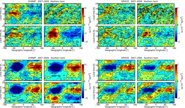
Figure 1.Local time versus longitudinal distribution of thermospheric mass density for four seasons in the Northern (top) and Southern (bottom) hemispheres both from CHAMP (left) and GRACE (right) observations.
vided into four seasons, centered around the March equinox, June solstice, September equinox, and December solstice. For each season overlapping periods of 131 and 161 days are needed to cover all 24 local time hours for CHAMP and GRACE, respectively. Days with planetary geomagnetic ac-tivity index (Ap) of>30 are excluded to reduce the influence of sever magnetic disturbances. The observations presented here are averages of the seasons over 3 years. Therefore, the results favor those tides which remain steady over long time. Tides occurring occasionally will not contribute much to the signals presented here.
3.1 Tidal features of the mass density at midlatitudes
As we discussed above, the longitudinal wave structures ob-served by near-polar orbiting satellites can be caused by many different tidal components. By analyzing the propa-gating phase of the wave in local time, different tidal com-ponents can be separated. For each season, the mass den-sity observations (ρ) is first sorted into MLAT (1◦) and geo-graphic longitude (15◦) bins. Then, the mass density between
±40 to±60◦MLAT is averaged for each local time hour. To suppress the migrating tides the longitudinal mean value is subtracted hour by hour.
Figure 1 presents the local time versus longitudinal dis-tribution of 1ρ for four seasons in the Northern (top) and
Southern (bottom) hemispheres both from CHAMP (left) and GRACE (right) mass density observations. Here1ρ means that the longitudinal mean value ofρhas been subtracted. At CHAMP altitude 1ρ is found to be largest throughout the year around 150–30◦W during 12:00–21:00 LT (except for the June solstice) in the Northern Hemisphere, while in the Southern Hemisphere a minimum value of1ρappears in the same longitude region during the same local time. The peak value of1ρin the Southern Hemisphere appears around 30– 150◦E during 12:00–21:00 LT, which is about 180◦apart in
longitude from the1ρpeak in the Northern Hemisphere. In-terestingly, a mixture of longitudinal wave structures can be seen in the Northern Hemisphere during the June solstice. In the Southern Hemisphere during the December solstice, a second peak appears around 150–30◦W during 21:00– 09:00 LT. The two peaks can be considered as part of a wave-1 pattern, which is consistent with our earlier report about the wave-1 pattern of the southern MSNA feature (Xiong and Lühr, 2014).
The mass density at GRACE altitude exhibits mixtures of longitudinal wave structures in the Northern Hemisphere during the four seasons, the peak value of1ρ around 150– 30◦W during 12:00–21:00 LT is only prominent during the
Tides
CHAMP 2007−2009 Northern hemi Mar. E.
D S T
SP June. S
Wavenumber
Tides
Sep. E.
−3 −2 −1 0 1 2 3 4 5 6 7 D S T SP Wavenumber Dec. S.
−3 −2 −1 0 1 2 3 4 5 6 7
Amplitude [10
−
1
4 kg/m 3] 0 0.5 1 1.5 2 2.5 3 Tides
GRACE 2007−2009 Northern hemi Mar. E.
D S T
SP June. S
Wavenumber
Tides
Sep. E.
−3 −2 −1 0 1 2 3 4 5 6 7 D S T SP Wavenumber Dec. S.
−3 −2 −1 0 1 2 3 4 5 6 7
Amplitude [10
−
1
4 kg/m 3] 0 0.1 0.2 0.3 0.4 0.5 Tides
CHAMP 2007−2009 Southern hemi Mar. E.
D S T
SP June. S
Wavenumber
Tides
Sep. E.
−3 −2 −1 0 1 2 3 4 5 6 7 D S T SP Wavenumber Dec. S.
−3 −2 −1 0 1 2 3 4 5 6 7
Amplitude [10
−
1
4 kg/m 3] 0 0.5 1 1.5 2 2.5 3 Tides
GRACE 2007−2009 Southern hemi Mar. E.
D S T
SP June. S
Wavenumber
Tides
Sep. E.
−3 −2 −1 0 1 2 3 4 5 6 7 D S T SP Wavenumber Dec. S.
−3 −2 −1 0 1 2 3 4 5 6 7
Amplitude [10
−
1
4 kg/m 3] 0 0.1 0.2 0.3 0.4 0.5
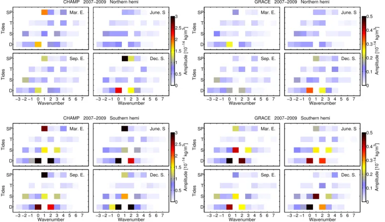
Figure 2.Spectra of the tidal and stationary components in mass density for four seasons in the Northern (top) and Southern (bottom) hemispheres both from CHAMP (left) and GRACE (right) observations.
12:00–21:00 LT. The larger value of1ρ around 150–30◦W during 21:00–09:00 LT throughout the whole year makes the wave-1 pattern much more prominent in the Southern Hemi-sphere at GRACE altitude, compared to that at CHAMP alti-tude.
Figure 2 presents the amplitudes of the full non-migrating tidal and stationary spectrum for four seasons separately in the Northern (top) and Southern (bottom) hemispheres both from CHAMP (left) and GRACE (right) mass density observations. As can be seen, in the Northern Hemisphere SPW1 and D0 are found to be the most prominent stationary and tidal components throughout the year both at CHAMP and GRACE altitudes, but this is not so obvious around the June solstice. During the December solstice DW2 also shows comparable amplitudes. The semidiurnal tidal com-ponent SE2 is relatively large during the September equinox. In the Southern Hemisphere, spectral amplitudes are larger. SPW1, D0, and DW2 are found to be prominent through-out the whole year. The semidiurnal components SW1 and SW3 are also presented at all seasons with somewhat smaller amplitudes. Similar to the Northern Hemisphere, the tidal component SE2 shows comparable amplitudes during the September equinox in the Southern Hemisphere. To make it easier for the reader, the numerical values of amplitudes and
phases for the two most important diurnal and semidiurnal tidal components are listed in Table 1.
3.2 Tidal features of the zonal wind at midlatitudes
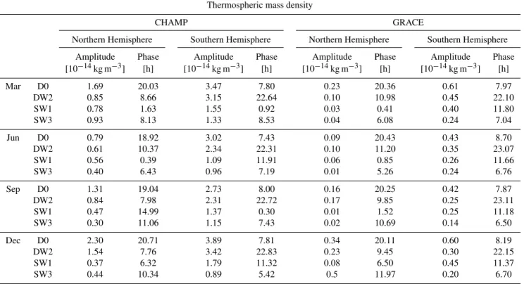
Table 1.Amplitudes and phases of diurnal tides D0 and DW2 as well as semidiurnal tides SW1 and SW3 from the thermospheric mass density measurements during the years 2007–2009.
Thermospheric mass density
CHAMP GRACE
Northern Hemisphere Southern Hemisphere Northern Hemisphere Southern Hemisphere
Amplitude Phase Amplitude Phase Amplitude Phase Amplitude Phase
[10−14kg m−3] [h] [10−14kg m−3] [h] [10−14kg m−3] [h] [10−14kg m−3] [h]
Mar D0 1.69 20.03 3.47 7.80 0.23 20.36 0.61 7.97
DW2 0.85 8.66 3.15 22.64 0.10 10.98 0.45 22.10
SW1 0.78 1.63 1.55 0.92 0.03 0.41 0.40 11.80
SW3 0.93 8.13 1.33 8.53 0.04 6.08 0.24 7.04
Jun D0 0.79 18.92 3.02 7.43 0.09 20.43 0.43 8.70
DW2 0.61 10.37 2.34 22.31 0.10 11.20 0.35 23.07
SW1 0.56 0.39 1.09 11.91 0.06 0.85 0.26 11.66
SW3 0.40 6.43 0.96 7.19 0.01 5.26 0.24 6.76
Sep D0 1.31 19.04 2.73 8.00 0.16 20.25 0.42 7.87
DW2 0.84 7.98 2.31 22.72 0.17 9.85 0.25 23.11
SW1 0.47 14.99 1.37 0.30 0.01 1.52 0.25 11.18
SW3 0.30 11.06 1.15 7.43 0.02 10.69 0.14 6.50
Dec D0 2.30 20.71 3.89 7.81 0.34 20.11 0.60 8.19
DW2 1.54 7.76 3.42 22.83 0.23 9.45 0.30 22.15
SW1 0.37 6.32 1.79 11.32 0.08 6.50 0.45 11.37
SW3 0.44 10.34 0.89 5.42 0.5 11.97 0.20 6.70
signatures in the electron and mass density, the amplitude of DW2 in zonal wind exceeds D0 during most of the seasons in both hemispheres (except the solstice seasons in the Southern Hemisphere). We will give a more detailed discussion about the tidal amplitudes and phases between the three quantities in the next section.
4 Discussion
The study presented here has provided the tidal signatures of the upper atmospheric mass density and zonal wind at midlatitudes for different seasons. Similar to the MSNA, as reported by Xiong and Lühr (2014), the in situ mass den-sity and zonal wind observations from CHAMP and GRACE at midlatitudes also exhibit prominent longitudinal wave-1 patterns in the Southern Hemisphere, especially during local summer. Since we consider the wind to be closely related to the driving mechanism, we will first discuss the features of the zonal wind.
4.1 Zonal wind observations and model predictions As already revealed by previous studies there are generally two major potential coupling mechanisms between the neu-tral atmosphere and the ionosphere. The first is upward prop-agation of non-migrating tides, since many of them are gen-erated in the troposphere and stratosphere due to latent heat release and planetary wave/migrating tide interactions
(Eng-land et al., 2010; Wu et al., 2012). Some of these tides can propagate directly to the upper thermosphere and generate the equally spaced patterns in longitude. The second is the E region wind dynamo. In this case, the non-migrating tides are not required to propagate all the way to the upper ther-mosphere, but electrodynamic coupling takes place between E and F regions, causing ion drifts at F region. As theE×B
drift mainly affects the F region at equatorial latitudes, it will not be important for the longitudinal wave patterns of the plasma at midlatitudes. However, the wave patterns of the MSNA as reported by Chen et al. (2013) and Xiong and Lühr (2014) imply that there should be some other coupling mechanism at midlatitudes. By model simulations, Jones Jr. et al. (2013) revealed that at low and middle latitudes the non-migrating tides of the zonal wind could be generated in situ through ion–neutral interactions due to the longitudinal iono-spheric density variations imposed by the actual geomagnetic field configuration. Their results also show that the primary non-migrating diurnal tides excited in situ by ion–neutral in-teraction at middle latitudes are D0 and DW2; the secondary semidiurnal tides are SW1 and SW3 (see their Fig. 5).
Local time [h]
CHAMP 2001−2003 Northern hemi
Mar. E.
0 6 12 18 24
June S.
Geographic longitude [°]
Local time [h]
Sep. E.
−1800 −90 0 90 180 6
12 18 24
Geographic longitude [°]
Dec. S.
−90 0 90 180
∆
zonal wind [m/s]
−75 −50 −25 0 25 50 75
Local time [h]
CHAMP 2001−2003 Southern hemi
Mar. E.
0 6 12 18 24
June S.
Geographic longitude [°]
Local time [h]
Sep. E.
−1800 −90 0 90 180 6
12 18 24
Geographic longitude [°]
Dec. S.
−90 0 90 180
∆
zonal wind [m/s]
−75 −50 −25 0 25 50 75
Figure 3.Local time versus longitudinal distribution of zonal wind for four seasons in the Northern (left) and Southern (right) hemispheres from CHAMP measurements.
Tides
CHAMP 2001−2003 Northern hemi Mar. E.
D S T
SP June. S
Wavenumber
Tides
Sep. E.
−3 −2 −1 0 1 2 3 4 5 6 7 D
S T SP
Wavenumber Dec. S.
−3 −2 −1 0 1 2 3 4 5 6 7
Amplitude [m/s]
0 5 10 15 20
Tides
CHAMP 2001−2003 Southern hemi Mar. E.
D S T
SP June. S
Wavenumber
Tides
Sep. E.
−3 −2 −1 0 1 2 3 4 5 6 7 D
S T SP
Wavenumber Dec. S.
−3 −2 −1 0 1 2 3 4 5 6 7
Amplitude [m/s]
0 5 10 15 20
Figure 4.Spectra of the tidal and stationary components in zonal wind from the Northern (left) and Southern (right) hemispheres from CHAMP measurements.
Jones Jr. et al. (2013) reported no phase values for compar-ison. They suggested a possible generation mechanism for the patterns in the wind that is based on an in situ interac-tion between the diurnal migrating tide DW1 and the stainterac-tion- station-ary planetstation-ary wave SPW1. Our result showed that the phase of the wind tidal components D0 and DW2 are rather simi-lar during all the seasons (see Table 2). This means that the sum of tidal signatures has extrema near 0 and 180◦longitude (cf. Fig. 3). Conversely, zero-crossing appears around±90◦. These are the longitudes towards which the magnetic dipole axis is tilted. Jones Jr. et al. (2013) clearly showed that the prominence of the wave-1 tides appear when the actual geo-magnetic field configuration is considered.
We use the same line of arguments to explain the promi-nent semidiurnal compopromi-nents SW1 and somewhat smaller SW3. In this case, it is the interaction of the migrating tide SW2 with SPW1. Jones Jr. et al. (2013) also predicted a prominent SW1 at middle latitudes and a smaller SW3. Also SW1 and SW3 vary practically in-phase and the two hemi-spheres vary again in anti-phase (6/12 h difference, see Ta-ble 2). Overall, our wind observations provide a good valida-tion of the presented simulavalida-tion results.
4.2 Comparison of mass density variations with ionospheric MSNA
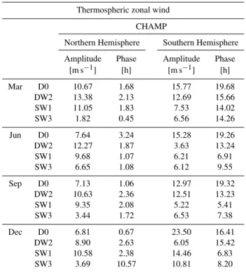
ob-Table 2.Same as Table 1, but for the CHAMP zonal wind measure-ments during the years 2001–2003.
Thermospheric zonal wind
CHAMP
Northern Hemisphere Southern Hemisphere
Amplitude Phase Amplitude Phase
[m s−1] [h] [m s−1] [h]
Mar D0 10.67 1.68 15.77 19.68
DW2 13.38 2.13 12.69 15.66
SW1 11.05 1.83 7.53 14.02
SW3 1.82 0.45 6.56 14.26
Jun D0 7.64 3.24 15.28 19.26
DW2 12.27 1.87 3.63 13.24
SW1 9.68 1.07 6.21 6.91
SW3 6.65 1.08 6.12 9.55
Sep D0 7.13 1.06 12.97 19.32
DW2 10.63 2.36 12.51 13.23
SW1 9.35 2.08 5.22 5.41
SW3 3.44 1.72 6.53 7.38
Dec D0 6.81 0.67 23.50 16.41
DW2 8.90 2.63 6.05 15.42
SW1 10.58 2.38 14.46 6.83
SW3 3.69 10.57 10.81 8.20
tain at CHAMP altitude for the Northern (Southern) Hemi-sphere a ratio of mass density of 0.06 (0.12). The related ratio for electron density at the Northern (Southern) Hemisphere is 0.34 (1.0) (see Table 1 of Xiong and Lühr, 2014). This result shows that compared to the electron density, the ef-fects of tide D0 in the thermospheric mass density is less by a factor of 6 to 8 at midlatitudes. As D0 is found to be the most prominent tidal component in both thermospheric mass density and electron density at midlatitudes; it may partly explain why the MSNA features can be seen directly in the F region electron density distribution, but not in the thermo-spheric mass density. Additionally, the interaction between the neutral wind and geomagnetic main field also contributes partly to the development of the ionospheric MSNA features. After subtracting the longitudinal mean, a coincidence of wave-1 structure in electron density, mass density as well as the zonal wind appears, implying that these non-migrating tides in the upper atmosphere are a result of a common driv-ing mechanism. We think that the ion–neutral interaction in the upper ionosphere, as described by Jones Jr. et al. (2013), is the primary cause.
As reported by Xiong and Lühr (2014), the northern MSNA shows a prominent eastward-propagating wave-2 pat-tern in electron density, and the dominating tidal and station-ary components are found to be DE1, SPW1, D0, and DW2 (ordered by magnitude). However, this wave-2 pattern can neither be found in the zonal wind nor in thermospheric mass density observations in the Northern Hemisphere. Therefore, we believe that additional interactions might exist, for
exam-ple, between the zonal wind and the geomagnetic field, addi-tionally controlling the distribution of electron density in the F region. Further studies are needed for clarifying the issue.
The amplitudes and phases of diurnal tidal components DE1, D0, and DW2, as well as semidiurnal components SW1 and SW2 from electron density observations are listed in Ta-ble 3. A closer phase comparison of the most prominent tidal components in the ionospheric and thermospheric annually averaged quantities is shown in Table 4. The most interest-ing is tide D0. It appears at very similar phases in both elec-tron and mass density, around 20:00 UT and 08:00 UT in the Northern and Southern hemispheres, respectively. This phase relationship for D0 in both neutral and ionization quanti-ties suggests that an upward and downward motion of the thermospheric background controls at least partly the varia-tion of electron density in the F region (see Xiong and Lühr, 2014). According to the Chapman layer formula, a larger at-mospheric scale height enhances the ionization rate. For the other tidal components we cannot find such a phase relation-ship between neutral and ionized constituents.
Another mechanism exciting the tidal components in mass density is the converging and diverging zonal wind. As ex-plained in the previous section, we find maxima of east-ward wind shortly after midnight in the Northern Hemi-sphere (Fig. 3). This implies a convergence and air upwelling around 90◦E in longitude as well as a divergence and down-welling around 90◦W. The opposite wind direction are in-ferred from the tidal components D0 and DW2 shortly after noon. Consistent with this notion, we found at CHAMP alti-tude in the Northern Hemisphere mass density enhancements around 90◦W and depletions around 90◦E shortly after noon
(Fig. 1). The opposite conditions prevail for density and wind in the Southern Hemisphere with mass density depletions around 90◦W and enhancement around 90◦E in longitude. This causal relationship suggest that the zonal wind is the main driver for the primary tides in mass density.
For completeness we want to comment on the appearance of the tide SE2 during the September equinox. This tidal component has earlier been observed (e.g., in thermospheric temperature at low-middle latitudes) and is related to wave-4 pattern caused by deep tropical convection in the troposphere (e.g., Oberheide et al., 2011a).
5 Summary
Based on accelerometer observations from CHAMP and GRACE satellites, tidal signatures of thermospheric mass density and zonal wind at midlatitudes have been analyzed in this study. The main results are summarized as follows:
Table 3.Same as Table 1, but for the electron density measurements during the years 2007–2009. The prominent diurnal tide DE1 has also been listed here.
Electron density
CHAMP GRACE
Northern Hemisphere Southern Hemisphere Northern Hemisphere Southern Hemisphere
Amplitude Phase Amplitude Phase Amplitude Phase Amplitude Phase [1010m−3] [h] [1010m−3] [h] [1010m−3] [h] [1010m−3] [h]
Mar DE1 1.44 2.15 0.86 10.02 0.47 2.18 0.32 8.34
D0 1.14 20.37 4.30 6.70 0.33 19.36 1.65 6.45
DW2 0.47 13.51 2.42 15.61 0.15 11.42 0.77 15.58
SW1 0.48 5.75 1.50 0.38 0.13 6.05 0.59 11.25
SW3 0.10 5.57 0.55 1.62 0.09 2.98 0.28 4.22
Jun DE1 2.02 2.28 0.10 0.12 0.66 2.37 0.04 16.56
D0 1.28 19.52 1.33 6.96 0.38 19.42 0.63 6.85
DW2 0.92 11.52 0.43 15.89 0.31 10.91 0.27 17.48
SW1 0.54 7.90 0.59 10.32 0.12 6.81 0.32 13.54
SW3 0.39 2.50 0.11 3.72 0.18 1.57 0.15 2.73
Sep DE1 1.45 1.82 0.92 9.42 0.42 2.13 0.32 8.18
D0 1.22 19.91 3.57 7.16 0.30 19.59 1.27 6.36
DW2 0.50 11.97 2.47 16.89 0.18 10.92 0.73 15.42
SW1 0.40 4.80 1.53 0.94 0.04 6.31 0.46 11.09
SW3 0.01 2.32 0.27 1.90 0.09 0.49 0.11 2.71
Dec DE1 0.85 2.27 2.19 9.97 0.25 2.46 0.67 9.03
D0 0.85 20.08 7.59 6.74 0.27 20.05 2.58 6.65
DW2 0.01 13.97 3.13 15.88 0.05 8.33 1.12 16.38
SW1 0.27 5.47 1.61 0.19 0.10 4.84 0.42 11.33
SW3 0.14 8.55 0.72 4.87 0.03 0.45 0.32 3.97
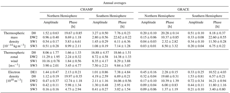
Table 4.Annual average values of the amplitudes and phases of the prominent diurnal and semidiurnal tides, in thermospheric mass density, zonal wind and electron density.
Annual averages
CHAMP GRACE
Northern Hemisphere Southern Hemisphere Northern Hemisphere Southern Hemisphere
Amplitude Phase Amplitude Phase Amplitude Phase Amplitude Phase
[h] [h] [h] [h]
Thermospheric D0 1.52±0.63 19.67±0.85 3.27±0.50 7.76±0.23 0.20±0.10 20.28±0.14 0.51±0.10 8.18±0.37 mass DW2 0.96±0.40 8.69±1.18 2.80±0.56 22.62±0.22 0.15±0.06 10.37±0.85 0.33±0.08 22.60±0.55 density SW1 0.54±0.17 5.83±6.61 1.45±0.29 6.11±6.36 0.04±0.03 2.32±2.82 0.34±0.10 11.50±0.28 [10−14kg m−3] SW3 0.51±0.28 8.99±2.11 1.08±0.19 7.14±1.28 0.03±0.01 8.50±3.32 0.20±0.04 6.75±0.22
Thermospheric D0 8.06±1.77 1.66±1.33 16.88±4.57 18.66±1.51 zonal DW2 11.29±1.95 2.24±0.32 8.72±4.58 14.38±1.33 wind SW1 10.16±0.78 1.84±0.56 8.35±4.17 8.29±3.88 [m s−1] SW3 3.90±2.01 3.45±4.77 7.50±2.21 9.84±3.07
Electron DE1 1.44±0.47 2.13±0.21 1.01±0.86 7.38±4.84 0.45±0.16 2.28±0.15 0.33±0.25 10.52±4.03 density D0 1.12±0.19 19.97±0.35 4.19±2.59 6.89±0.21 0.32±0.04 19.60±0.31 1.53±0.81 6.57±0.21 [1010m−3] DW2 0.47±0.37 12.74±1.18 2.11±1.16 16.06±0.56 0.17±0.10 10.39±1.39 0.72±0.34 16.21±0.94
of migrating tides, DW1 and SW2, with the stationary planetary wave, SPW1. The tides D0, DW2, SW1, and SW3 vary in anti-phase in the two hemispheres. This is believed to be due to the tilt of the magnetic dipole field. 2. The thermospheric mass density is also dominated by wave-1 longitudinal features. Again, the diurnal tides D0 and DW2 are strongest. The wave-1 semidiurnal components, SW1 and SW3, are also present but signif-icantly smaller. The phases of the diurnal tides exhibit an anti-phase relationship between the hemispheres. All phase values differ significantly from zonal wind phases, as expected.
3. We regard the thermospheric dynamics as the main driver for the electron density tidal structures. An exam-ple is the in-phase variation of D0 between electron den-sity and mass denden-sity in both hemispheres. DW2 shows similarities in amplitude between the two densities, but large differences in phase. The prominent wave-2 signa-ture, DE1, in the Northern Hemisphere electron density is quite puzzling, present neither in the mass density nor in the zonal wind. Further studies are needed for fully understanding these relationships.
Acknowledgements. The CHAMP and GRACE missions were sponsored by the Space Agency of the German Aerospace Center (DLR) through funds of the Federal Ministry of Economics and Technology. The CHAMP and GRACE thermospheric mass density data are available at the website of air den-sity models derived from multi-satellite drag observations (http://thermosphere.tudelft.nl/acceldrag/data.php). The work of Chao Xiong is supported by the Alexander von Humboldt founda-tion through a Research Fellowship for Postdoctoral Researchers. The work of Yun-Liang Zhou is supported by the National Nature Science Foundation of China (no. 41274194 and no. 40804049).
The service charges for this open-access publication have been covered by a Research Centre of the Helmholtz Association.
Topical Editor C. Jacobi thanks two anonymous referees for their help in evaluating this paper.
References
Bellchambers, W. H. and Piggott, W. R.: Ionospheric mea-surements made at Halley Bay, Nature, 182, 1596–1597, doi:10.1038/1821596a0, 1958.
Burns, A. G., Zeng, Z., Wang, W., Lei, J., Solomon, S. C., Rich-mond, A. D., Killen, T. L., and Kuo, Y.-H.: Behavior of the F2 peak ionosphere over the South Pacific at dusk during quiet summer condition from COSMIC data, J. Geophys. Res., 113, A12305, doi:10.1029/2008JA013308, 2008.
Chang, L. C., Lin, C.-H., Yue, J., Liu, J.-Y., and Lin, J.-T.: Stationary planetary wave and nonmigrating tidal signatures in ionospheric wave 3 and wave 4 variations in 2007–2011 FORMOSAT-3/COSMIC observations, J. Geophys. Res.-Space, 118, 6651–6665, doi:10.1002/jgra.50583, 2013.
Chapman, S. and Lindzen, R. S.: Atmospheric Tides: Thermal and Gravitational, D. Reidel Publishing Company, Dordrecht, Hol-land, 1970.
Chen, C. H., Lin, C. H., Chang, L. C., Huba, J. D., Lin, J. T., Saito, A., and Liu, J. Y.: Thermospheric tidal effects on the ionospheric midlatitude summer nighttime anomaly using SAMI3 and TIEGCM, J. Geophys. Res.-Space, 118, 3836–3845, doi:10.1002/jgra.50340, 2013.
Doornbos, E., Ijssel, J., Lühr, H., Förster, M., and Koppenwallner, G.: Neutral density and crosswind determination from arbitrarily oriented multiaxis accelerometers on satellites, J. Spacraft Rock-ets, 47, 580–589, doi:10.2514/1.48114, 2010.
Dudeney, J. R. and Piggott, W. R.: Antarctic ionospheric research, in: Upper Atmosphere Research in Antarctica, Antarct. Res. Ser., 29, edited by: Lanzerotti, L. J. and Park, C. G., 200–235, AGU, Washington, D. C., 1978.
England, S. L., Maus, S., Immel, T. L., and Mende, S. B.: Longitude variation of the E-region electric fields caused by atmospheric tides, Geophys. Res. Lett., 33, L21105, doi:10.1029/2006GL027465, 2006.
England, S. L., Immel, T. J., Huba, J. D., Hagan, M. E., Maute, A., and DeMajistre, R.: Modeling of multiple effects of atmo-spheric tides on the ionosphere: An examination of possible coupling mechanisms responsible for the longitudinal structure of the equatorial ionosphere, J. Geophys. Res., 115, A05308, doi:10.1029/2002JA009262, 2010.
Forbes, J. M.: Tidal and Planetary Waves, in: The upper Mesosphere and Lower Thermosphere: A Review of Experiment and The-ory, Geophysical Monograph, 87, edited by: Johnson, R. M. and Killeen, T. L., AGU, 1995.
Forbes, J. M., Zhang, X., Ward, W., and Talaat, E.: Nonmigrating diurnal tides in the thermosphere, J. Geophys. Res., 108, 1033, doi:10.1029/2009JA014894, 2003.
Forbes, J. M., Russell, J., Miyahara, S., Zhang, X., Palo, S., Mlynczak, M., Mertens, C. J., and Hagan, M. E.: Troposphere-thermosphre tidal coupling as measured by the SABER instru-ment on TIMED during July–September 2002, J. Geophys. Res., 111, A10S06, doi:10.1029/2005JA011492, 2006.
Hagan, M. E. and Forbes, J. M.: Migrating and nonmigrating diurnal tides in the middle and upper atmosphere excited by tropospheric latent heat release, J. Geophys. Res., 107, 4754, doi:10.1029/2001JD001236, 2002.
Hagan, M. E. and Forbes, J. M.: Migrating and nonmigrating semidiurnal tides in the upper atmosphere excited by tro-pospheric latent heat release, J. Geophys. Res., 108, 1062, doi:10.1029/2002JA009466, 2003.
Hagan, M. E. and Roble, R. G.: Modeling the diurnal tidal vari-ability with the National Center for Atmospheric Research thermosphere-ionosphere-mesosphere-electrodynamics general circulation model, J. Geophys. Res., 106, 24869–24882, doi:10.1029/2001JA000057, 2001.
Häusler, K. and Lühr, H.: Nonmigrating tidal signals in the up-per thermospheric zonal wind at equatorial latitudes as observed by CHAMP, Ann. Geophys., 27, 2643–2652, doi:10.5194/angeo-27-2643-2009, 2009.
He, M., Liu, L., Wan, W., Ning, B., Zhao, B., Wen, J., Yue, X., and Le, H.: A study of the Weddell Sea Anomaly observed by FORMOSAT-3/COSMIC, J. Geophys. Res., 114, A12309, doi:10.1029/2009JA014175, 2009.
Immel, T. J., Sagawa, E., England, S. L., Henderson, S. B., Ha-gan, M. E., Mende, S. B., Frey, H. U., Swenson, C. M., and Paxton, L. J.: Control of equatorial ionospheric morphol-ogy by atmospheric tides, Geophys. Res. Lett., 33, L15108, doi:10.1029/2006GL026161, 2006.
Jones Jr., M., Forbes, J. M., Hagan, M. E., and Maute, A.: Non-migrating tides in the ionosphere-thermosphere: In situ versus tropospheric sources, J. Geophys. Res.-Space, 118, 2438–2451, doi:10.1002/jgra.50257, 2013.
Kil, H., Paxton, L. J., Lee, W. K., Ren, Z., Oh, S.-J., and Kwak, Y.-S.: Is DE2 the source of the ionospheric wavenum-ber 3 longitudinal structure?, J. Geophys. Res., 115, A11319, doi:10.1029/2010JA015979, 2010.
Lin, C. H., Liu, J. Y., Cheng, C. Z., Chen, C. H., Liu, C. H., Wang, W., Burns, A. G., and Lei, J.: Three-dimensional ionospheric electron density structure of the Weddell Sea Anomaly, J. Geo-phys. Res., 114, A02312, doi:10.1029/2008JA013455, 2009. Lin, C. H., Liu, C. H., Liu, J. Y., Chen, C. H., Burns, A. G., and
Wang, W.: Midlatitude summer nighttime anomaly of the iono-spheric electron density observed by FORMOSAT-3/COSMIC, J. Geophys. Res., 115, A03308, doi:10.1029/2009JA014084, 2010.
Liu, H., Lühr, H., Watanabe, S., Köhler, W., Henize, V., and Visser, P.: Zonal winds in the equatorial upper thermo-sphere: Decomposing the solar flux, geomagnetic activity, and seasonal dependencies, J. Geophys. Res., 111, A07307, doi:10.1029/2005JA011415, 2006.
Liu, H., Yamamoto, M., and Lühr, H.: Wave-4 pattern of the equatorial mass density anomaly: A thermospheric signature of tropical deep convection, Geophys. Res. Lett., 36, L18104, doi:10.1029/2009GL039865, 2009.
Liu, H., Thampi, S. V., and Yamamoto, M.: Phase reversal of the diurnal cycle in the midlatitude ionosphere, J. Geophys. Res., 115, A01305, doi:10.1029/2009JA014689, 2010.
Lühr, H. and Manoj, C.: The complete spectrum of the equatorial electrojet related to solar tides: CHAMP observations, Ann. Geo-phys., 31, 1315–1331, doi:10.5194/angeo-31-1315-2013, 2013. Lühr, H., Rother, M., Häusler, K., Alken, P., and Maus, S.: The
influence of non-migrating tides on the longitudinal variation of the equatorial electrojet, Geophys. Res. Lett., 113, A08313, doi:10.1029/2008JA013064, 2008.
Lühr, H., Rother, M., Häusler, K., Fejer, B., and Alken, P.: Direct comparison of non-migrating tidal signatures in the electrojet, vertical plasma drift and equatorial ionization anomaly, J. Atmos. Sol.-Terr. Phy., 75–76, 31–43, doi:10.1016/j.jastp.2011.07.009, 2012.
McLandress, C. and Ward, W. E.: Tidal/gravity wave interactions and their influence on the large-scale dynamics of the middle atmosphere: Model results, J. Geophys. Res., 99, 8139–8155, doi:10.1029/94JD00486, 1994.
Oberheide, J., Hagan, M. E., Roble, R. G., and Offermann, D.: Sources of nonmigrating tides in the tropical middle atmosphere, J. Geophys. Res., 107, 4567, doi:10.1029/2002JD002220, 2002. Oberheide, J., Forbes, J. M., Häusler, K., Wu, Q., and Bruinsma, S. L.: Tropospheric tides from 80 to 400 km: Propagation, interan-nual variability, and solar cycle effects, J. Geophys. Res., 114, D00I05, doi:10.1029/2009JD012388, 2009.
Oberheide, J., Forbes, J. M., Zhang, X., and Bruinsma, S. L.: Wave-driven variability in the ionosphere-thermosphere-mesosphere system from TIMED observations: What con-tributes to the “wave 4”?, J. Geophys. Res., 116, A01306, doi:10.1029/2010JA015911, 2011a.
Oberheide, J., Forbes, J. M., Zhang, X., and Bruinsma, S. L.: Climatology of upward propagating diurnal and semidiurnal tides in the thermosphere, J. Geophys. Res., 116, A01306, doi:10.1029/2011JA016784, 2011b.
Pancheva, D., Miyoshi, Y., Mukhtarov, P., Jin, H., Shinagawa, H., and Fujiwara, H.: Global response of the ionosphere to atmospheric tides forced from below: Comparison be-tween COSMIC measurements and simulations by atmosphere-ionosphere coupled model GAIA, J. Geophys. Res., 117, A07319, doi:10.1029/2011JA017452, 2012.
Penndorf, R.: The average ionospheric conditions over the Antarc-tic, in Geomagnetism and Aeronomy, Antarct. Res. Ser., 4, 1–45, AGU, Washington, D.C., 1965.
Reigber, C., Lühr, H., and Schwintzer, P.: CHAMP mission status, Adv. Space Res., 30, 129–134, 2002.
Rishbeth, H.: The effect of winds on the ionospheric F2-peak, J. Atmos. Terr. Phys., 29, 225–238, doi:10.1016/0021-9169(67)90192-4, 1967.
Rishbeth, H.: The effect of winds on the ionospheric F2-peak-II, J. Atmos. Terr. Phys., 30, 63–71, doi:10.1016/0021-9169(68)90041-X, 1968.
Sagawa, E., Immel, T. J., Frey, H. U., and Mende, S. B.: Lon-gitudinal structure of the equatorial anomaly in the nighttime ionosphere observed by IMAGE/FUV, J. Geophys. Res., 110, A11302, doi:10.1029/2004JA010848, 2005.
Tapley, B. D., Bettadpur, S., Watkins, M., and Reigber, C.: The gravity recovery and climate experiment: Mission overview and early results, Geophys. Res. Lett., 31, L09607, doi:10.1029/2004GL019920, 2004.
Thampi, S. V., Lin, C., Liu, H., and Yamamoto, M.: First tomographic observations of the midlatitude summer night-time anomaly over Japan, J. Geophys. Res., 114, A10318, doi:10.1029/2009JA014439, 2009.
Wan, W., Xiong, J., Ren, Z., Liu, L., Zhang, M.-L., Ding, F., Ning, B., Zhao, B., and Yue, X.: Correlation between the ionospheric WN4 signature and the upper atmospheric DE3 tide, J. Geophys. Res., 115, A11303, doi:10.1029/2010JA015527, 2010.
Wu, Q., Ortland, D. A., Foster, B., and Roble, R. G.: Simulation of nonmigrating tide influences on the thermosphere and iono-sphere with a TIMED data driven TIEGCM, J. Atmos. Sol.-Terr. Phy., 90–91, 61–67, doi:10.1016/j.jastp.2012.02.009, 2012. Xiong, C. and Lühr, H.: Nonmigrating tidal signatures in the
magnitude and the inter-hemispheric asymmetry of the equa-torial ionization anomaly, Ann. Geophys., 31, 1115–1130, doi:10.5194/angeo-31-1115-2013, 2013.
as tidal features, J. Geophys. Res.-Space, 119, 4905–4915, doi:10.1002/2014JA019959, 2014.
Xiong, C., Lühr, H., and Stolle, C.: Seasonal and latitudinal variations of the electron density nonmigrating tidal spec-trum in the topside ionospheric F-region as resolved from CHAMP observations, J. Geophys. Res.-Space, online first, doi:10.1002/2014JA020354, 2014a.