ABSTRACT: The breeze potential along the Brazilian northern and northeastern coast was studied using wind data from the Climate Forecast System Reanalysis for the period between 1980 and 2010. March and September were considered, which are representative of the rainy and dry (or less rainy) periods, respectively. The Brazilian northern and northeastern coast is composed by meridionally oriented coastlines (Amapá State coast and eastern coast of Northeast Brazil) and a zonally oriented coastline (Brazilian northern coast east of Marajó Island). Along the meridionally oriented coastlines, the breeze potential was mainly related to the zonal wind and extended inland over 1 – 2° from the shore. The daily zonal wind cycle maximum (minimum), which represents the land (sea) breeze potential, occurred at ~0700 UTC (~1900 UTC). Along the zonally oriented coastline, the breeze potential was mainly related to the meridional wind and extended inland and offshore over 2 – 3° from the shore. At the shore, the daily meridional wind cycle maximum (minimum), which represents the land (sea) breeze potential, occurred at ~1000 UTC (~2200 UTC). Phase propagation occurred from the shore inland in March and September and also offshore in September. In general, for the entire Brazilian northern and northeastern coast, the breeze potential frequency was higher in September (20 – 25 days per month). In March, while the frequency slightly decreased over the meridionally oriented coastlines (to 15 – 20 days per month), the frequency sharply decreased over the zonally oriented coastlines to 5 – 10 days per month in landside coastal areas and vanished in seaside coastal areas. Higher frequency was generally related to lower interannual variability, and there was signiicant correlation between the interannual variability of the frequency and oceanic indices, along speciic coastal areas. The features of the breeze potential areas obtained in this study complement the results from others and provide a more complete depiction of breeze features along the entire Brazilian northern and northeastern coast.
KEYWORDS: Land-sea breeze, Coastal breeze, Brazilian coast, Surface wind, Daily cycle.
Breeze Potential Along the Brazilian
Northern and Northeastern Coast
Dayana Castilho de Souza1, Marcos Daisuke Oyama2
INTRODUCTION
In coastal regions, breeze is an important and widely studied phenomenon (Simpson 1994; Miller et al. 2003). It generally consists of land-sea breezes, particularly over areas near the coastline, but also includes mountain-valley breezes over the transition between coastal and inland elevated areas and lake/ river breezes over water bodies (such as bays and river mouths) at landside coastal regions. Land-sea breezes are thermally direct shallow cells driven by horizontal pressure gradients set up by the diferential heating of contiguous land and water surfaces, and are frequently observed in tropical regions due to the strong solar heating and weak Coriolis force (Yan and Anthes 1987). he intensity of land-sea breezes is afected by the large scale circulation (Estoque 1962; Laird et al. 2001) and regional factors, such as land use (Miao et al. 2003; Kala et al.
2010) and coastline shape (McPherson 1970; Baker et al. 2001). Breeze in the Brazilian northern and northeastern (BNNE) coast (Fig. 1a) is addressed in this study. he main climatological features of this coastal region are described by Kayano and Andreoli (2009), Marengo and Nobre (2009), and Reboita et al.
(2010). he low-level circulation predominantly originates from the Atlantic Ocean and varies between southeasterly and northeasterly. he annual precipitation ranges from 1,500 to 2,000 mm; the average surface temperature, from 24 to 28 °C. he rainy (dry or less rainy) season occurs in the irst (last) 6 months of the year. he main large-scale system related to the seasonal precipitation maximum is the Intertropical Convergence Zone. he BNNE coast consists of the Amapá State and eastern coasts, which are meridionally-oriented coastlines, as well as the northern coast, which is a zonally-oriented coastline (Fig. 1b).
1.Instituto de Pesquisas Espaciais – Centro de Previsão de Tempo e Estudos Climáticos – Cachoeira Paulista/SP – Brazil. 2.Departamento de Ciência e Tecnologia Aeroespacial – Instituto de Aeronáutica e Espaço – Divisão de Ciências Atmosféricas – São José dos Campos/SP – Brazil.
Author for correspondence: Marcos Daisuke Oyama | Departamento de Ciência e Tecnologia Aeroespacial – Instituto de Aeronáutica e Espaço – Divisão de Ciências
Atmosféricas | Praça Marechal Eduardo Gomes, 50 – Vila das Acácias | CEP: 12.228-904 – São José dos Campos/SP – Brazil | Email: [email protected]
The current knowledge of the areas affected by breeze circulations along locations at or parts of the BNNE coast, as revealed by studies that focus on and identify breeze circulations observationally, is summarized in Fig. 1a. Areas afected by land-sea breezes are precisely mapped only for the northern coastal areas east of São José Bay (delineated by dotted and dashed lines in Fig. 1a). Over these areas, it is usually possible to track the diurnal inland propagation of sea breeze fronts using visible satellite images; on average, these fronts reach approximately 40 to 80 km inland (Planchon et al. 2006), and this extent includes areas where the land-sea breeze signature is found in the surface wind daily cycle (Barreto et al. 2002). he maximum ofshore propagation of land breeze fronts can also be found using early morning visible satellite images; on average, these fronts reach approximately a few degrees ofshore (Teixeira 2008), and this extent agrees with estimates based on QuikSCAT scatterometer wind data (Gille et al. 2005). For the other parts of the northern coast, observational evidence of breeze circulations based on wind data are reported for only 2 locations: Alcântara (Medeiros and Fisch 2012) and Belém (land-sea and river breezes: Santos et al. 2012).
he eastern coast is another region for which some breeze features are known. Due to persistent low-level cloudiness, it is not possible to clearly identify the breeze fronts over this region (Planchon et al. 2006). herefore, breeze features are found using the daily surface wind cycle. According to Barreto
et al. (2002), generally, land-sea breezes are found over landside coastal areas, while mountain-valley breezes are increasingly common further inland. This is verified by studies on the speciic locations at the States of Paraíba, Pernambuco and Alagoas, shown in Fig. 1a (Gomes Filho et al. 1990; Bento and Cavalcanti 1994; Nóbrega et al. 2000; Rocha and Lyra 2000; Costa and Lyra 2012).
Although previous studies have mapped the areas afected by breeze circulations in parts of the BNNE coast, there are still large unmapped regions, such as the northern coast west of São José Bay (except at Alcântara and Belém), the Amapá coast and the southern part of the eastern coast. his study aims to map the areas afected by breeze circulations for the entire BNNE coast, thus complementing the indings from previous studies. Due to the lack of a dense observational network in this region with available data for long periods (Brito 2013), the
Figure 1. (a) Political map of Brazil. The BNNE coast extends between the 2 black illed circles and is indicated by the double arrow line. The areas (locations) inluenced by breezes, according to the literature, are shaded (represented by open circles). LSB: Land-sea breeze; MVB: Mountain-valley breeze; RLB: River/lake breeze. The sea (land) breeze extent is represented by dashed (dotted) lines. The location of Belém (Pará State) and Alcântara (Maranhão State) is shown. (b) Parts of the BNNE coast: Amapá and eastern coasts (meridionally-oriented coastlines, red dashed line) as well as northern coast (zonally-oriented coastline, blue dashed line). The 2 open circles refer to the PI-point (1) and PE-point (2). The region between Marajó Bay and São José Bay is enlarged to show the numerous bays along the coastline and the approximate location of the Amazon River.
Numerous bays
Amapá coast
Northern coast
Marajó Island Marajó Bay
Amazon River 1
2
São Marcos Bay São José Bay
Eastern coast
A: Teixeira (2008) B: Gille et al. (2005) CE: Ceará PA: Pará AP: Amapá MA: Maranhão PI: Piauí BA: Bahia SE: Sergipe
RN: Rio Grande do Norte PB: Paraíba
PE: Pernambuco AL: Alagoas
PA AP
MA CE PI
BA SE AL
PE PB RN
A B
Alcântara Belém
LSB and MVB or MVB only LSB only
LSB and RLB
(a)
new generation of reanalysis products known as the Climate Forecast System Reanalysis (CFSR; Saha et al. 2010) is used. Besides the important and common features of all reanalysis datasets, such as global coverage, long temporal range and data availability, the CFSR data have higher spatial resolution (grid spacing of 0.5°) and temporal frequency (hourly data). Although this grid spacing does not allow for an accurate representation of local breeze circulations, the hourly frequency is suitable for the identification of breezes, and the temporal range (1979 – present) allows for deriving climatological information.
Due to the limitation related to the horizontal resolution, the CFSR data allows for mapping the areas with what is named here as “breeze potential”. his is a new term that refers to the integrated result of the various types of breezes on the surface wind signal at a regional scale. While actual breeze fronts could propagate over tens of kilometers (e.g., Planchon et al.
2006), breeze potential refers to a quasi-stationary cloudiness over few hundred kilometers from the coastline (Souza 2016). herefore, the areas with breeze potential are usually larger than and include those afected by actual breeze circulations.
he identiication of actual breezes demands the existence of a clear and numerically coherent relationship between land-sea thermal gradients and intradaily wind changes (assuming negligible forcing from larger scale transient systems). However, this relationship does not always hold along the BNNE coast (e.g., Planchon et al. 2006). herefore, for the sake of simplicity, as in numerous other studies (e.g., Gille et al. 2003), only wind data are considered here to obtain the areas with breeze potential, because a pronounced daily surface wind cycle is a necessary condition for the occurrence of actual breezes (Ferreira et al. 2006)
Therefore, this study aims specifically to delimit the continental and oceanic areas with the breeze potential for the entire BNNE coast. Additionally, for these areas, a simple method to identify the days with breeze potential is proposed, the climatology of the breeze potential frequency using this method is obtained, and a preliminary analysis on the interannual variability of the frequency (its degree and relation with oceanic indices) is carried out.
DATA AND METHODOLOGY
CLIMATE FORECAST SYSTEM REANALYSIShe CFSR dataset was developed by the National Centers for Environmental Prediction (Saha et al. 2010). Hourly data
(analysis at 00, 06, 12 and 18 UTC, and forecasts at the remainder hours) at a regular 0.5° × 0.5° global grid from 1979 to the present are available from the website at http://rda.ucar.edu. he higher resolution and other improvements implemented to derive the CFSR dataset led to the correction of errors mainly in the Southern Hemisphere (e.g., Silva et al. 2011; Quadro
et al. 2012). For Alcântara, Souza (2016) found good agreement between wind proiles from the CFSR and radiosonde data.
To examine the breeze potential along the BNNE coast, hourly zonal and meridional wind data at 1000 hPa from the CFSR for 2 contrasting months — September and March — over 31 years (1980 – 2010) are used. September is chosen because it represents the dry (or less rainy) season in the Amapá and northern coasts; March, because it represents the rainy season in major parts of the BNNE coast. he areas with breeze potential, in general, attain maximum (minimum) extent during the dry (rainy) season, because less (more) cloudiness leads to higher (lower) land-sea thermal gradients. herefore, the months of September and March would represent the upper and lower limits of the breeze potential occurrence. he zonal and meridional wind components are used without projecting them into other directions, because the meridional (zonal) wind is nearly perpendicular to the zonally-/meridionally-oriented coastline(s), and land-sea breeze circulations develop perpendicularly to the coast.
HARMONIC ANALYSIS
Harmonic analysis (Wilks 2011) is applied to the hourly time series of the wind components separately for March and September of each year. he amplitude/phase of the harmonic related to the daily cycle and the proportion of the explained variance are computed. Areas where this harmonic explains more than 1/3 of the variance for at least 1/3 of the total number of years are considered to be with breeze potential. his threshold (1/3) ensures the continuity of areas with breeze potential (as suggested in Fig. 1a) without extending them far inland (in general, extent < 300 km) (Souza 2016). For the sake of simplicity, the same threshold is adopted for the proportion of explained variance and the number of years.
WAVELET TRANSFORM
a periodic function (in time) modulated by a Gaussian function (Eq. 1 from Torrence and Compo 1998), is used as the basis function. he level of signiicance (section 4 of Torrence and Compo 1998) is deined as 95%.
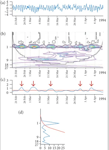
An illustration of the full WT output is given in Fig. 2. he WT decomposes the signal in time and scale (frequency), and results in the wavelet power spectrum (Fig. 2b), which allows for picking out the time intervals when higher power within a scale of interest (cycle or variability) is found. he time average
of the wavelet power spectrum for each scale produces the global wavelet spectrum (Eq. 22 of Torrence and Compo 1998; Fig. 2d), which is equivalent to the Fourier transform spectrum. he average within a scale interval (band) results in the time series of the scale-averaged wavelet power (SAWP; Eq. 24 of Torrence and Compo 1998; Fig. 2c). For the band related to the daily cycle, higher (lower) SAWP values correspond to a greater (lesser) contribution of the daily cycle to the signal variability. Here, SAWP ≥ 0.5 is assumed to be the exact condition for the occurrence of the breeze potential on a daily basis.
CONTINGENCY TABLE STATISTICS
To obtain a simple procedure to identify the occurrence of breeze potential on a daily basis, 2 methods are objectively compared using 2 × 2 contingency table statistics. he statistics are: critical success index [CSI = a/(a + b + c)], hit rate [H = a/(a+ c)], false alarm ratio [FAR = b/(a + b)] and bias [B = (a + b)/(a + c)], where a is the number of hits; b, false alarms; c, misses; and d, correct rejections (Wilks 2011). Perfect agreement occurs when b = c = 0; in this case, CSI = H = B = 1, and FAR = 0.
INTERANNUAL VARIABILITY DEGREE AND OCEANIC INDICES
For each wind component (zonal or meridional wind) of a given month (March or September), the yearly time series of the breeze potential frequency is composed by 31 values from 1980 to 2010 (each frequency value refers to the number of days with breeze potential for the given month and year).
• he average (μ) and standard deviation (δ) are computed from the 31 values. he degree of interannual variability of the breeze potential frequency is measured by the coeicient of variation (CV), which is the ratio between
δ and μ (CV = δ/μ).
• The yearly time series of frequency is correlated (with lag 0) to 2 oceanic indices related to the climate variability in Northeast Brazil (Kayano and Andreoli 2009): the Niño 3 index (NINO3) for the tropical Paciic and the interhemispheric sea surface temperature anomaly gradient (GRAD) for the tropical Atlantic. he deinition of the indices follows Andreoli and Kayano (2007), and computation details are given in Marques and Oyama (2015). Pearson’s correlation coeicient above 0.30 means statistical signiicance at the 90% conidence level.
Figure 2. Illustration of the WT output. The WT is applied to the detrended and normalized time series (a) of the meridional wind for the PI-point in March 1994. The WT decomposes the signal in time (horizontal axis of panels a, b and c) and scale (vertical axis of panels b and d, given in days) and results in the wavelet power spectrum (b). Red contours indicate high power, and signiicant power values are enclosed by black lines. The time average of the wavelet power for each scale results in the global wavelet spectrum (d). Most of the power is concentrated on the single signiicant peak (above the red line) at the 1-day scale. The average within the scale interval (band) of interest — here, the band related to the daily cycle — results in the time series of the SAWP (c). In panel c, the periods when SAWP ≥ 0.5 (condition for the occurrence of breeze potential on a daily basis) are indicated by red downward arrows.
4
1994 2
0 –2 –4
21 F
eb
26 F
eb
1 Ma
r
6 Ma
r
11 M
ar
16 M
ar
21 M
ar
26 M
ar
1 Ap
r
6 Ap
r
1
1994 9
18 27
21 F
eb
26 F
eb
1 Ma
r
6 Ma
r
11 M
ar
16 M
ar
21 M
ar
26 M
ar
1 Ap
r
6 Ap
r
1994 0
1 2 3
21 F
eb
26 F
eb
1 Ma
r
6 Ma
r
11 M
ar
16 M
ar
21 M
ar
26 M
ar
1 Ap
r
6 Ap
r
25 27
18 9 1
20 15 10 5 0 (a)
(b)
(c)
RESULTS
AREAS WITH BREEZE POTENTIAL
For September, the breeze potential is generally found in the zonal wind over the meridionally-oriented coastlines (eastern and Amapá coasts) (Fig. 3a), and in the meridional wind over the zonally-oriented coastline (northern coast) (Fig. 3b). For some regions, such as the Ceará State shore, breeze potential is found in both wind components. he breeze potential is not restricted to coastal areas and can extend far inland. For these inner continental areas, located few degrees from the coastline, the breeze potential (which refers to the integrated result of the various types of breezes) may not represent the land-sea breeze, but may be either related to mountain-valley breeze, as is the case in the central region of the Maranhão State (Fig. 3a), or to river/lake breeze, as is the case over the Amazon River in the Pará State (Fig. 3b).
Analyzing the zonal wind along the meridionally-oriented coastlines, the areas with breeze potential are generally limited by the 150 and 500 m height contour lines in the Amapá and eastern coasts, respectively (Fig. 3a). In these areas, the daily zonal wind cycle maximum occurs at 0500 – 0900 UTC (~sunrise; Fig. 3c). his maximum represents the land breeze potential (positive or westerly zonal wind). he minimum, which represents the sea breeze potential, occurs at 1700 – 2100 UTC, i.e., 12 h ater the maximum (~sunset; negative or easterly zonal wind). Slight phase propagation is found over areas with breeze potential. his pattern of land-sea breeze potential resembles the results of observational studies on land-sea breezes for the region (e.g., Gomes Filho et al. 1990; Costa and Lyra 2012).
Based on the analysis of the meridional wind along the zonally-oriented coastline, the areas with breeze potential
extend inland and ofshore (Fig. 3b). In the Maranhão State, the continental areas with breeze potential are limited by the 150 m height contour line. The spatial pattern of the daily meridional wind cycle maximum shows marked phase propagation from the coastline (Fig. 3d). At the coastline, the maximum, which represents the land breeze potential (positive or southerly meridional wind), occurs at 0900 – 1100 UTC, while the minimum, which represents the sea breeze potential (negative or northerly meridional wind), occurs at 2100 – 2300 UTC. From the coastline, extending inland and ofshore, the maximum and minimum occur at progressively later hours. he ofshore phase propagation agrees with Gille et al. (2005) and Teixeira (2008); the inland phase propagation agrees with Planchon et al. (2006).
For March, the areas with breeze potential are similar to those mapped for September, although the areas related to the meridional wind are only continental and more spatially conined (Fig. 4). In the zonally-oriented coastline, the ofshore propagation disappears, and the inland propagation extends over shorter distances.
he areas with breeze potential for March or September are summarized in Fig. 5. his map delimits the areas with breeze potential in at least 1 month (March or September). Inland areas further than 3° from the coastline are excluded because the present study focuses on coastal areas. Along the zonally-/meridionally-oriented coastline(s), the breeze potential extends inland and ofshore (inland) over 2 – 3° (1 – 2°) from the coastline. For the Ceará coast, the 2 – 3° extent is well above the observed inland sea breeze propagation (40 – 80 km, according to Planchon et al. 2006), but it agrees with the ofshore land breeze propagation (Gille et al. 2005; Teixeira 2008).
Figure 3. (a and b) Elevation map (m) with blue lines enclosing the areas with breeze potential in September; (c and d) Phase (UTC hour when the wind component value is positive and maximum) for these areas. Panels a and c refer to the zonal wind (Uvel); panels b and d refer to the meridional wind (Vvel).
10N UvelSep
5N EQ
5S
10S
15S 20S
60W 55W 50W 45W 40W 35W 30W
10N
500 200 150 100 50 Vvel
Sep 5N
EQ 5S
10S
15S 20S
60W 55W 50W 45W 40W 35W 30W
10N UvelSep
5N EQ
5S
10S
15S 20S
60W 55W 50W 45W 40W 35W 30W
10N VvelSep
5N
23 21 19 17 15 13 11 9 7 5 3 1 EQ
5S
10S
15S 20S
60W 55W 50W 45W 40W 35W 30W
Some inland discontinuities in the breeze potential are found over the region between Marajó Island and São José Bay. his may be due to the presence of numerous bays along the coastline (Fig. 1b), which could give rise to complex and intense local circulation patterns, but to a weak (spatially) integrated response (therefore, to a weak breeze potential).
IDENTIFICATION OF BREEZE POTENTIAL OCCURRENCE ON A DAILY BASIS
To map the areas with breeze potential, harmonic analysis of the wind data was used. his method, however, could not be applied to verify the breeze potential occurrence for any given day because it uses all of the records of the time series. herefore, a new method for the occurrence of breeze potential is derived. The method is adjusted for the following two CFSR grid points (Fig. 1b): the PI-point and the PE-point. The
PI-point (PE-point) is regarded as representative of the zonally-/meridionally-oriented coastline(s). For the PI-point (PE-point), the meridional (zonal) wind is analyzed. Data for March and September of 3 contrasting years (1994, 2008 and 2010) are used. For the northern coast, the proportion of the explained variance by the daily cycle is generally below, around and above the average in 1994, 2008 and 2010, respectively (for the eastern coast, it is generally above the average for all these years). For each point, the WT is applied to the time series of the wind component for a given month and year. For both points, the only signiicant peak in the global wavelet spectrum occurs at the scale related to the daily cycle (for instance, see Fig. 2).
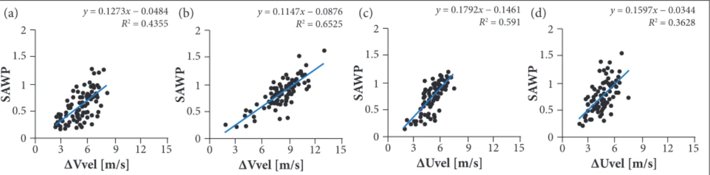
Firstly, as mentioned previously, SAWP ≥ 0.5 is assumed to be the exact condition for the occurrence of breeze potential on a daily basis. This condition is consistent with the criteria used to define the areas with breeze potential, but it cannot be used for real-time monitoring (because, for a given day, data for the subsequent days are needed to compute the WT using the Morlet wavelet as basis function). Therefore, a simpler method, based on the relationship between SAWP and the daily amplitude of the wind component (∆), is derived. SAWP and D are correlated linearly and positively, and the coefficient of determination (R2) ranges from 36 to 65% (Fig. 6), which indicates an acceptable regression for geophysical signals. By considering this relationship and using the standard deviation of the wind component (σ) as a scaling parameter for each location, the new method for identification of the occurrence of breeze potential on a daily basis is written as shown by Eq.1:
Figure 4. (a and b) Elevation map (m) with blue lines enclosing the areas with breeze potential in March; (c and d) Phase (UTC hour when the wind component value is positive and maximum) for these areas. Panels a and c refer to the zonal wind (Uvel); panels b and d refer to the meridional wind (Vvel).
10N UvelMar
5N EQ
5S
10S
15S 20S
60W 55W 50W 45W 40W 35W 30W 10N
500 200 150 100 50 Vvel
Mar 5N
EQ 5S
10S
15S 20S
60W 55W 50W 45W 40W 35W 30W
10N UvelMar
5N EQ
5S
10S
15S 20S
60W 55W 50W 45W 40W 35W 30W
10N VvelMar
5N
23 21 19 17 15 13 11 9 7 5 3 1 EQ
5S
10S
15S 20S
60W 55W 50W 45W 40W 35W 30W
Figure 5. Areas with breeze potential in March or September (shaded).
10N
5N
EQ
5S
10S
15S
20S
60W 55W 50W 45W 40W 35W 30W
where amin is a threshold.
(a) (b) (c) (d)
h e threshold is calibrated by comparing the days with SAWP ≥ 0.5 (Figs. 7 and 8) and a ≥ amin, through the use of 2 × 2 contingency table statistical measures. he inal value of
amin is 2.4 (which is also valid in July for Alcântara according to Souza 2016), except in the case of meridional wind in March, when amin is 3.3. Using these calibrated values, there is a relative
Figure 6. Relationship between the daily amplitude of the wind component and SAWP. Meridional wind (∆Vvel) and PI-point for March (a) and September (b); zonal wind (∆Uvel) and PE-point for March (c) and September (d). In each panel, the regression line, the line equation and the coeficient of determination (R2) are shown.
Figure 8. SAWP time series of the meridional wind at the PI-point (left panels) and the zonal wind at the PE-point (right panels) for September in 1994, 2008 and 2010. SAWP values are computed for the band related to the daily cycle. The red line refers to SAWP = 0.5.
Figure 7. SAWP time series of the meridional wind at the PI-point (left panels) and the zonal wind at the PE-point (right panels) for March in 1994, 2008 and 2010. SAWP values are computed for the band related to the daily cycle. The red line refers to SAWP = 0.5.
PI-point, meridional wind, September
3 1994 26 A ug 21 A ug 2 1 0 1 S ep 6 S ep 11 S ep 16 S ep 21 S ep 26 S ep 1 O ct 6 O ct 26 A ug 21 A ug 1 S ep 6 S ep 11 S ep 16 S ep 21 S ep 26 S ep 1 O ct 6 O ct 26 A ug 21 A ug 1 S ep 6 S ep 11 S ep 16 S ep 21 S ep 26 S ep 1 O ct 6 O ct 3 2008 2 1 0 3 2010 2 1 0
PE-point, zonal wind, September
3 1994 26 A ug 21 A ug 2 1 0 1 S ep 6 S ep 11 S ep 16 S ep 21 S ep 26 S ep 1 O ct 6 O ct 26 A ug 21 A ug 1 S ep 6 S ep 11 S ep 16 S ep 21 S ep 26 S ep 1 O ct 6 O ct 26 A ug 21 A ug 1 S ep 6 S ep 11 S ep 16 S ep 21 S ep 26 S ep 1 O ct 6 O ct 3 2008 2 1 0 3 2010 2 1 0
PI-point, meridional wind, March PE-point, zonal wind, March
3 1994 6 Ap r 1 Ap r 26 M ar 21 M ar 16 M ar 11 M ar 6 Ma r 1 Ma r 26 F eb 21 F eb 2 1 0 3 2008 6 Ap r 1 Ap r 27 M ar 22 M ar 17 M ar 12 M ar 7 Ma r 2 Ma r 26 F eb 21 F eb 2 1 0 3 2010 6 Ap r 1 Ap r 26 M ar 21 M ar 16 M ar 11 M ar 6 Ma r 1 Ma r 26 F eb 21 F eb 2 1 0 3 1994 6 Ap r 1 Ap r 26 M ar 21 M ar 16 M ar 11 M ar 6 Ma r 1 Ma r 26 F eb 21 F eb 2 1 0 3 2008 6 Ap r 1 Ap r 27 M ar 22 M ar 17 M ar 12 M ar 7 Ma r 2 Ma r 26 F eb 21 F eb 2 1 0 3 2010 6 Ap r 1 Ap r 26 M ar 21 M ar 16 M ar 11 M ar 6 Ma r 1 Ma r 26 F eb 21 F eb 2 1 0 0 0 0.5 1 1.5 2
3 6 9 12 15
∆Vvel [m/s]
SA
W
P
y = 0.1273x − 0.0484
R2 = 0.4355
0 0 0.5 1 1.5 2
3 6 9 12 15
∆Vvel [m/s]
SA
W
P
y = 0.1147x − 0.0876
R2 = 0.6525
0 0 0.5 1 1.5 2
3 6 9 12 15
∆Uvel [m/s]
SA
W
P
y = 0.1792x − 0.1461
R2 = 0.591
0 0 0.5 1 1.5 2
3 6 9 12 15
∆Uvel [m/s]
SA
W
P
y = 0.1597x − 0.0344
R2 = 0.3628
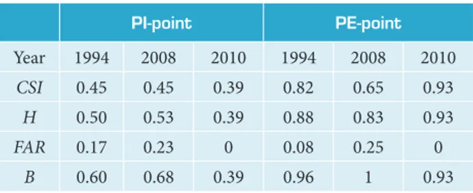
good agreement between the methods for both months (Tables 1 and 2). In general, the CSI and H statistics are high, FAR is low and B is near 1. he agreement is rather poor for the PI-point in March, but is quite good in September. For the PE-point, the agreement is slightly better in March.
Along the zonally-oriented coastline, the results for the meridional wind data are analyzed:
• In March (Fig. 9b), the breeze potential frequency is low (5 – 10 days per month) and restricted to landside coastal areas. Since the average frequency is low, the interannual variability is not analyzed for this month.
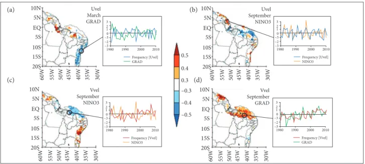
• In September (Fig. 9d), the frequency is higher along landside coastal areas (20 – 25 days per month) and decreases ofshore (~15 days per month). he interannual variability of the frequency, however, is higher along seaside coastal areas (CV of 25 – 50%) and decreases inland (CV of 10 – 25%; not shown). he variability is signiicantly correlated to GRAD for both landside and seaside coastal areas (Fig. 10d) and to NINO3 only for the latter (Fig. 10c). he time series from 2 gridpoints in the northern coast illustrates that La Niña (El Niño) conditions over the tropical Paciic and northward (southward) GRAD over the tropical Atlantic tend to increase (decrease) the breeze potential frequency.
Along the meridionally-oriented coastlines, the results for the zonal wind data are analyzed, and only landside coastal areas are considered, because those with breeze potential do not extend ofshore (Fig. 5):
• In March, the frequency is 15 – 20 days per month (Fig. 9a), and CV ranges from 10 to 50% (not shown). Along the eastern coast, the interannual variability of the frequency is signiicantly correlated with GRAD (Fig. 10a). he time series from a particular gridpoint in the eastern coast illustrates that southward (northward) GRAD over the tropical Atlantic tend to increase (decrease) the breeze potential frequency. he interannual
PI-point PE-point
Year 1994 2008 2010 1994 2008 2010
CSI 0.88 0.96 0.93 0.65 0.80 0.78
H 0.92 0.96 0.93 0.71 0.95 0.81
FAR 0.04 0 0 0.11 0.17 0.05
B 0.96 0.96 0.93 0.79 1.14 0.85
Table 1. Contingency table statistics from the comparison between the 2 methods of breeze potential identiication (SAWP ≥ 0.5 and a ≥ amin) for March.
PI-point PE-point
Year 1994 2008 2010 1994 2008 2010
CSI 0.45 0.45 0.39 0.82 0.65 0.93
H 0.50 0.53 0.39 0.88 0.83 0.93
FAR 0.17 0.23 0 0.08 0.25 0
B 0.60 0.68 0.39 0.96 1 0.93
Table 2. Contingency table statistics from the comparison between the 2 methods of breeze potential identiication (SAWP ≥ 0.5 and a ≥ amin) for September.
BREEZE POTENTIAL FREQUENCY
Using the method based on Eq. 1, the climatology of the breeze potential frequency in March and September for the period between 1980 and 2010 is obtained. A preliminary analysis on the interannual variability of the frequency for regions with higher average frequency (≥ 15 days per month) is also carried out.
10N UvelMar
5N EQ
5S
10S
15S 20S
60W 55W 50W 45W 40W 35W 30W
10N
30 28 29 15 12 10 5 3 1 Vvel Mar 5N
EQ
5S
10S
15S 20S
60W 55W 50W 45W 40W 35W 30W
10N UvelSep
5N EQ
5S
10S
15S 20S
60W 55W 50W 45W 40W 35W 30W
10N VvelSep
5N 30
25 20 15 12 10 5 3 1 EQ
5S
10S
15S 20S
60W 55W 50W 45W 40W 35W 30W
Figure 9. The average breeze potential frequency (number of days per month) in March (a and b) and September (c and d) for the areas shaded in Fig. 3. The left-side panels (a and c) refer to the climatology obtained using the zonal wind data (Uvel); the right-side panels (b and d) refer to the climatology obtained using the meridional wind data (Vvel).
variability along the Amapá coast could not be explained by the oceanic indices. Significant correlation with NINO3 is restricted to isolated gridpoints (not shown).
• In September, the frequency increases to 20 – 25 days per month (Fig. 9c), and the degree of interannual variability is lower (CV of 10 – 25%; not shown). Along the Amapá coast, the interannual variability of the frequency is signiicantly correlated with NINO3 (Fig. 10b). he time series from a particular gridpoint in the Amapá coast illustrates that El Niño (La Niña) conditions over the tropical Paciic tend to increase (decrease) the breeze potential frequency. Along the eastern coast, signiicant correlation with NINO3 is found in areas close to the shoreline. Significant correlation with GRAD is restricted to isolated gridpoints (not shown). herefore, for the entire BNNE coast, the breeze potential frequency would be generally higher in the dry (or less rainy) period (e.g., September). In the rainy period (e.g., March), while the frequency would slightly decrease over the meridionally-oriented coastlines, it would sharply decrease over the zonally-oriented coastline and vanish over seaside coastal areas. For regions with frequency above 15 days per month, higher frequency is generally related to lower interannual variability, and the relation between interannual variability
10N
15S 10S 5S EQ 5N
Uvel March GRAD
20S
60W 55W 50W 45W 40W 35W 30W
10N
15S 10S 5S
EQ 5N
Vvel September NINO3
20S
60W 55W 50W 45W 40W 35W 30W
10N
15S 10S 5S EQ 5N
Uvel September NINO3
20S
60W 55W 50W 45W 40W 35W 30W
10N
15S 10S 5S EQ 5N
Vvel September GRAD
20S
60W 55W 50W 45W 40W 35W 30W
0.5
0.4
0.3 –0.3
–0.4
–0.5
1980 –3 –2 –30 1 2 3
1990 2000 2010
Frequency [Uvel] GRAD
1980 –3 –2 –30 1 2 3
1990 2000 2010
Frequency [Uvel] NINO3
1980 –3 –2 –3 0 1 2 3
1990 2000 2010
Frequency [Vvel] GRAD 1980
–3 –2 –30 1 2 3
1990 2000 2010
Frequency [Vvel] NINO3
Figure 10. Correlation between the breeze potential frequency and oceanic indices (NINO3 and GRAD). The color key refers to the Pearson’s correlation coeficient, and absolute values above 0.3 are statistically signiicant at the 90% conidence level. In each panel, the time series of the normalized frequency for a speciic gridpoint (black) and the normalized oceanic index (red) are also shown. Uvel: Zonal wind; Vvel: Meridional wind. (a) March, correlation between GRAD and frequency from Uvel; (b) September, correlation between NINO3 and frequency from Uvel; (c) September, correlation between NINO3 and frequency Vvel; (d) September, correlation between GRAD and frequency from Vvel.
of the frequency and oceanic indices could be summarized as follows. In March, southward GRAD over the tropical Atlantic would increase the breeze potential frequency along the eastern coast. In September, while La Niña conditions over the tropical Paciic would increase the frequency along seaside areas of the northern coast and decrease along the Amapá coast, northward GRAD would increase the frequency along the northern coast.
CONCLUDING REMARKS
In this study, the breeze potential along the BNNE coast was studied using wind data from the CFSR for the period between 1980 and 2010. March and September were considered for being representative of the rainy and dry (or less rainy) periods, respectively. hese months would represent the upper and lower limits of the breeze potential occurrence.
Along the meridionally-oriented coastlines, the breeze potential was mainly related to the zonal wind and extended inland over 1 – 2° from the shore. he daily zonal wind cycle maximum (minimum), which represents the land (sea) breeze potential, occurred at ~0700 UTC (~1900 UTC). Along the zonally-oriented coastline, the breeze potential was mainly related to the meridional wind and extended inland and ofshore over 2 – 3° from the shore.
(a)
(c)
(b)
At the shore, the daily meridional wind cycle maximum (minimum), which represents the land (sea) breeze potential, occurred at ~1000 UTC (~2200 UTC). From the shore extending inland (and also offshore in September), the maximum and minimum occurred at progressively later hours (phase propagation). he areas with breeze potential obtained here complement the results from previous studies (summarized in Fig. 1a) and provide a more complete depiction of breeze features along the entire BNNE coast.
Additionally, to identify the breeze potential occurrence on a daily basis, a simple method based on the daily wind amplitude was derived (Eq. 1). Applying this method, the breeze potential frequency in March and September was obtained. In general, for the entire BNNE coast, the breeze potential frequency was higher in September (20 – 25 days per month). In March, while the frequency slightly decreased over the meridionally oriented coastlines (to 15 – 20 days per month), the frequency sharply decreased over the zonally-oriented coastlines (to 5 – 10 days per month in landside coastal areas and vanished in seaside coastal areas). herefore, the frequency would be higher in the dry (or less rainy) period.
For regions with higher breeze potential frequency (> 15 days per month), a preliminary analysis showed that higher frequency is generally related to lower interannual variability, and there is signiicant correlation between the interannual variability of the frequency and oceanic indices along speciic coastal areas. For instance, in March, southward
GRAD would increase the frequency along the eastern coast; in September, El Niño conditions would increase the frequency along the Amapá coast, and northward GRAD would increase the frequency along the northern coast.
Future study could focus on the propagation of sea breeze fronts along speciic coastal areas using satellite images (Planchon
et al. 2006; Lensky and Dayan 2012) and high-resolution simulations (Souza 2016), concerning the relation between breeze potential frequency and synoptic conditions (Laird et al.
2001) as well as other factors (e.g., the large-scale low-level circulation; Marques and Oyama 2015) that afect the interannual variability of the frequency.
ACKNOWLEDGEMENTS
he irst author was supported by grants from the Coor-denação de Aperfeiçoamento de Pessoal de Nível Superior (CAPES) and the Conselho Nacional de Desenvolvimento Cientíico e Tecnológico (CNPq). he authors are grateful to the 2 anonymous reviewers for their useful comments.
AUTHOR’S CONTRIBUTION
his paper is part of Souza DC’s doctoral thesis under the guidance of Oyama MD.
REFERENCES
Andreoli RV, Kayano M (2007) A importância relativa do Atlântico Tropical Sul e Pacíico Leste na variabilidade de precipitação do Nordeste do Brasil. Rev Bras Meteorol 22(1):63-74. doi: 10.1590/S0102-77862007000100007
Baker RD, Lynn BH, Boone A, Tao WK, Simpson J (2001) The inluence of soil moisture, coastline curvature, and land-breeze circulations on sea-breeze initiated precipitation. J Hydrometeor 2(2):193-211. doi: 10.1175/1525-7541(2001)002<0193:TIOSMC>2.0.CO;2
Barreto AB, Silva Aragão MR, Braga CC (2002) Estudo do ciclo diário do vento à superfície no Nordeste do Brasil. Proceedings of the 12th Brazilian Congress of Meteorology; Foz do Iguaçu, Brazil.
Bento PB, Cavalcanti EP (1994) Comportamento do vento à superfície na Paraíba e correlação com outras estações do Nordeste do Brasil. Proceedings of the 8th Brazilian Congress of Meteorology; Belo Horizonte, Brazil.
Brito SSB (2013) Diurnal cycle of precipitation over northern Brazil (PhD thesis). São José dos Campos: Instituto Nacional de Pesquisas Espaciais. In Portuguese.
Costa GB, Lyra RFF (2012) Wind patterns analysis in Alagoas State. Rev Bras Meteorol 27(1):31-38. doi: 10.1590/S0102-77862012000100004
Estoque MA (1962) The sea breeze as a function of the prevailing synoptic situation. J Atmos Sci 19(3):244-250. doi: 10.1175/1520-0469(1962)019<0244:TSBAAF>2.0.CO;2
Ferreira AD, Lemes MAM, Rodrigues LRL (2006) Variabilidade intra-anual do vento para a cidade de Maceió, AL, Brasil, em 2004: análise espectral. Proceedings of the 14th Brazilian Congress of Meteorology; Florianópolis, Brazil.
Gille ST, Llewellyn Smith SG, Lee SM (2003) Measuring the sea breeze from QuikSCAT Scatterometry. Geophys Res Lett 30(3):11-14. doi: 10.1029/2002GL016230
Gille ST, Llewellyn Smith SG, Statom NM (2005) Global observations of the land breeze. Geophys Res Lett 32:L05605. doi: 10.1029/2004GL022139
Kala J, Lyons TJ, Abbs D, Nair US (2010) Numerical simulations of the impacts of land-cover change on a southern sea breeze in south-west south-western Australia. Boundary-Layer Meteorology 135(3):485-503. doi: 10.1007/s10546-010-9486-z
Kayano MT, Andreoli RV (2009) Clima da região nordeste do Brasil. In: Cavalcanti IFA, Ferreira NJ, Justi da Silva MGA, Silva Dias MAF, editors. Tempo e clima no Brasil. São Paulo: Oicina de Textos. p. 213-233.
Laird NF, Kristovich DAR, Liang XZ, Arritt RW, Labas K (2001) Lake Michigan Lake Breezes: climatology, local forcing, and synoptic environment. J Appl Meteor 40(3):409-424. doi: 10.1175/1520-0450(2001)040<0409:LMLBCL>2.0.CO;2
Lensky IM, Dayan U (2012) Continuous detection and characterization of the Sea Breeze in clear sky conditions using Meteosat Second Generation. Atmos Chem Phys 12(14):6505-6513. doi: 10.5194/ acp-12-6505-2012
Marengo JA, Nobre CA (2009) Clima de região Amazônica. In: Cavalcanti IFA, Ferreira NJ, Justi da Silva MGA, Silva Dias MAF, editors. Tempo e clima no Brasil. São Paulo: Oicina de Textos. p. 197-214.
Marques RFC, Oyama MD (2015) Interannual variability of precipitation for the Centro de Lançamento de Alcântara in ENSO-neutral years. J Aerosp Technol Manag 7(3):365-373. doi: 10.5028/jatm.v7i3.477
McPherson RD (1970) A numerical study of the effect of a coastal irregularity on the sea breeze. J Appl Meteor 9(5):767-777. doi: 10.1175/1520-0450(1970)009<0767:ANSOTE>2.0.CO;2
Medeiros LE, Fisch G (2012) Low atmospheric low at Centro de Lançamento de Alcântara (CLA) and surrounding areas of the north part of Maranhão state. Proceedings of the 17th Brazilian Congress of Meteorology; Gramado, Brazil.
Miao JF, Kroon LJM, Vilà-Gerau de Arellano J, Holtslag B (2003) Impacts of topography and land degradation on the sea breeze over eastern Spain. Meteorol Atmos Phys 84(3):157-170. doi: 10.1007/ s00703-002-0579-1
Miller STK, Keim BD, Talbot RW, Mao H (2003) Sea breeze: structure, forecasting, and impacts. Rev Geophys 41(3):10-11. doi: 10.1029/2003RG000124
Nóbrega RS, Melo ECS, Araújo JAP, Paiva Neto AC, Soares DB (2000) Um estudo observacional de vento à superfície na cidade de Campina Grande-PB. Proceedings of the 11th Brazilian Congress of Meteorology; Rio de Janeiro, Brazil.
Planchon O, Damato F, Dubreuil V, Gouery P (2006) A method of identifying and locating sea-breeze fronts in north-eastern Brazil by remote sensing. Meteorol Appl 13(3):225-234. doi: 10.1017/ S1350482706002283
Quadro MFL, Silva Dias MAF, Herdies DL, Gonçalves LGG (2012) Climatological analysis of the precipitation and humidity transport on the SACZ region using the new generation of reanalysis. Rev Bras Meteorol 27(2):152-162. doi: 10.1590/S0102-77862012000200004
Reboita MS, Gan MA, Rocha RP, Ambrizzi T (2010) Precipitation regimes in South America: a bibliography review. Rev Bras Meteorol 25(2):185-204. doi: 10.1590/S0102-77862010000200004
Rocha CHED, Lyra RFF (2000) Ocorrência de brisas na região de tabuleiros costeiros próximo a Maceió-AL. Proceedings of the 11th Brazilian Congress of Meteorology; Rio de Janeiro, Brazil.
Saha S, Moorthi S, Pan HL, Wu X, Wang J, Nadiga S, Tripp P, Kistler R, Woollen J, Behringer D et al. (2010) The NCEP Climate Forecast System Reanalysis. Bull Amer Meteor Soc 91(8):1015-1057. doi: 10.1175/2010BAMS3001.1
Santos SRQ, Vitorino MI, Braga CC, Campos TLOB, Santos APP (2012) The effect of sea breeze over Belém-PA using multivariate analysis. Rev Bras Geogr Fis 5(5):1110-1120.
Silva VBS, Kousky VE, Higgins RW (2011) Daily precipitation statistics for South America: an intercomparison between NCEP reanalysis and observations. J Hydrometeor 12(1):101-117. doi: 10.1175/2010JHM1303.1
Simpson JE (1994) Sea breeze and local wind. New York: Cambridge University Press.
Souza DC (2016) Breeze in northern and eastern coast of Brazil (PhD thesis). São José dos Campos: Instituto Nacional de Pesquisas Espaciais. In Portuguese.
Teixeira RFB (2008) The breeze phenomenon and its relationship with the rain over Fortaleza-CE. Rev Bras Meteorol 23(3):282-291. doi: 10.1590/S0102-77862008000300003
Torrence C, Compo GP (1998) A practical guide to wavelet analysis. Bull Amer Meteor Soc 79(1):61-78. doi: 10.1175/1520-0477(1998)079<0061:APGTWA>2.0.CO;2
Wilks DS (2011) Statistical methods in the atmospheric sciences. 3rd edition. San Diego: Academic Press.