www.hydrol-earth-syst-sci.net/20/257/2016/ doi:10.5194/hess-20-257-2016
© Author(s) 2016. CC Attribution 3.0 License.
Time series of tritium, stable isotopes and chloride reveal short-term
variations in groundwater contribution to a stream
C. Duvert1, M. K. Stewart2, D. I. Cendón3,4, and M. Raiber5
1Queensland University of Technology, Brisbane, QLD 4001, Australia
2Aquifer Dynamics Ltd & GNS Science, P.O. Box 30368, Lower Hutt, 5040, New Zealand 3Australian Nuclear Science and Technology Organisation, Kirrawee DC, NSW 2232, Australia
4School of Biological, Earth & Environmental Sciences, University of New South Wales, Sydney, NSW 2052, Australia 5CSIRO Land & Water, Dutton Park, Brisbane, QLD 4102, Australia
Correspondence to:C. Duvert ([email protected])
Received: 23 July 2015 – Published in Hydrol. Earth Syst. Sci. Discuss.: 18 August 2015 Revised: 9 November 2015 – Accepted: 11 December 2015 – Published: 18 January 2016
Abstract.A major limitation to the assessment of catchment transit time (TT) stems from the use of stable isotopes or chloride as hydrological tracers, because these tracers are blind to older contributions. Yet, accurately capturing the TT of the old water fraction is essential, as is the assessment of its temporal variations under non-stationary catchment dy-namics. In this study we used lumped convolution models to examine time series of tritium, stable isotopes and chlo-ride in rainfall, streamwater and groundwater of a catchment located in subtropical Australia. Our objectives were to de-termine the different contributions to streamflow and their variations over time, and to understand the relationship be-tween catchment TT and groundwater residence time. Stable isotopes and chloride provided consistent estimates of TT in the upstream part of the catchment. A young component to streamflow was identified that was partitioned into quickflow (mean TT ≈2 weeks) and discharge from the fractured ig-neous rocks forming the headwaters (mean TT≈0.3 years). The use of tritium was beneficial for determining an older contribution to streamflow in the downstream area. The best fits between measured and modelled tritium activities were obtained for a mean TT of 16–25 years for this older ground-water component. This was significantly lower than the resi-dence time calculated for groundwater in the alluvial aquifer feeding the stream downstream (≈76–102 years), emphasis-ing the fact that water exitemphasis-ing the catchment and water stored in it had distinctive age distributions. When simulations were run separately on each tritium streamwater sample, the TT of old water fraction varied substantially over time, with values
averaging 17±6 years at low flow and 38±15 years after major recharge events. This counterintuitive result was inter-preted as the flushing out of deeper, older waters shortly after recharge by the resulting pressure wave propagation. Overall, this study shows the usefulness of collecting tritium data in streamwater to document short-term variations in the older component of the TT distribution. Our results also shed light on the complex relationships between stored water and wa-ter in transit, which are highly non-linear and remain poorly understood.
1 Introduction
history of the tracer input in rainfall-derived recharge water. Interpretation of TT data is often problematic because a sin-gle sample typically contains water parcels with different recharge histories, different flowpaths to the stream and thus different ages. This is exacerbated when the catchment is un-derlain by heterogeneous aquifers, as dispersion and mixing of different water sources can lead to very broad spectra of ages (Weissmann et al., 2002). Rather than a single scalar value, samples are therefore characterised by a TT distribu-tion (i.e. probability density funcdistribu-tion of the TTs contained in the sample). The residence time (RT) distribution is another useful indicator that refers to the distribution of ages of water resident within the system, rather than exiting it. RT distribu-tions are generally used to characterise subsurface water or deeper groundwater that is stored in the catchment.
In the last 2 decades, a great deal of effort has been di-rected to the determination of catchment TTs in a variety of streams and rivers worldwide (e.g. Maloszewski et al., 1992; Burns et al., 1998; Soulsby et al., 2000; Rodgers et al., 2005; Dunn et al., 2010). Attempts have been made to cor-relate the TTs to catchment characteristics such as topogra-phy (McGuire et al., 2005; Mueller et al., 2013; Seeger and Weiler, 2014), geology (Katsuyama et al., 2010) or soil type (Tetzlaff et al., 2009, 2011; Timbe et al., 2014). Assessment of the relationship between groundwater RT and catchment TT has also been undertaken occasionally (Matsutani et al., 1993; Herrmann et al., 1999; Reddy et al., 2006). Because catchment storage is highly non-stationary, catchment TTs are known to vary over time (McDonnell et al., 2010), yet the importance of temporal dynamics in TT distributions has been overlooked until recently. One of the reasons is that this non-stationarity is not accounted for in the models com-monly used in catchment TT research. In the last 5 years, an ever-growing number of studies has transferred its focus to assessing dynamic TT distributions (Hrachowitz et al., 2010, 2013; Roa-García and Weiler, 2010; Rinaldo et al., 2011; Cvetkovic et al., 2012; Heidbüchel et al., 2012, 2013; McMillan et al., 2012; Tetzlaff et al., 2014; Birkel et al., 2015; van der Velde et al., 2015; Benettin et al., 2015; Har-man, 2015; Klaus et al., 2015a; Kirchner, 2015). Most of these studies agreed on the importance of considering stor-age dynamics, because the RT distribution of storstor-age water and the TT distribution of water transiting at the outlet of the catchment are likely to be very different. Concurrently to these recent advances in catchment hydrology, groundwa-ter scientists have also developed new theoretical bases for the incorporation of transient conditions in RT distribution functions (Massoudieh, 2013; Leray et al., 2014). Nonethe-less, the determination of time-variant TT and RT distribu-tions requires data-intensive computing, which still largely limits their use in applied studies (Seeger and Weiler, 2014). A simple, yet still widely used alternative to more sophis-ticated models is the lumped-parameter modelling approach, which has been developed since the 1960s to interpret age tracer data (Vogel, 1967; Eriksson, 1971; Maloszewski and
Zuber, 1982). Lumped models require minimal input infor-mation, and are based on the assumptions that the shape of the TT or RT distribution function is a priori known and that the system is at steady state. The relationship between input and output signatures is determined analytically using a con-volution integral, i.e. the amount of overlap of the TT or RT distribution function as it is shifted over the input function. Some of the lumped models consider only the mechanical advection of water as driver of tracer transport (e.g. expo-nential model), while others also account for the effects of dispersion–diffusion processes (e.g. dispersion model). Non-parametric forms of RT distribution functions have recently been developed (Engdahl et al., 2013; Massoudieh et al., 2014b; McCallum et al., 2014), but again, these more re-cent approaches require a higher amount of input data, which makes the standard lumped-parameter approach a method of choice for the time being.
Commonly used to determine TT distributions using such models are the stable isotopes of water (δ2H andδ18O).
Be-cause they are constituents of the water molecule itself,2H
and 18O follow almost the same response function as the
traced material, hence are generally referred to as “ideal” tracers. Another tracer that behaves relatively conservatively and has been often used in the literature is chloride. An im-portant issue with using2H,18O and/or chloride as TT
indi-cators is that detailed catchment-specific input functions are needed (ideally at a weekly sampling frequency for several years), and such data are rare globally. More importantly, Stewart et al. (2010, 2012) criticised the use of these trac-ers to assess catchment TTs, arguing that TT distributions are likely to be truncated when only2H and/or18O are used.
In an earlier study, Stewart et al. (2007) reported differences of up to an order of magnitude between the TTs determined using stable isotopes as compared to those determined using tritium (3H). Later works by Seeger and Weiler (2014) and
Kirchner (2015) reinforced the point that “stable isotopes are effectively blind to the long tails of TT distributions” (Kirch-ner, 2015). The effects of older groundwater contributions to streamflow have largely been ignored until recently (Smer-don et al., 2012; Frisbee et al., 2013), and according to Stew-art et al. (2012), new research efforts need to be focused on relating deeper groundwater flow processes to catchment re-sponse. Accounting for potential delayed contributions from deeper groundwater systems therefore requires the addition of a tracer, such as3H, that is capable of determining longer
TTs.
3H is a radioactive isotope of hydrogen with a half-life
of 12.32 years. Like 2H and 18O it is part of the water
molecule and can therefore be considered an “ideal” tracer. Fractionation effects are small and can be ignored relative to measurement uncertainties and to its radioactive decay (Michel, 2005). The bomb pulse3H peak that occurred in the
con-centrations of remnant bomb pulse water have now decayed well below that of modern rainfall (Morgenstern and Daugh-ney, 2012). These characteristics allow the detection of rela-tively older groundwater (up to 200 years) and, importantly, the calculation of unique TT distributions from a single 3H
value, provided the measurement is accurate enough (Mor-genstern et al., 2010; Stewart et al., 2010). Other age trac-ers such as chlorofluorocarbons and sulfur hexafluoride have shown potential for estimating groundwater RT (e.g. Cook and Solomon, 1997; Lamontagne et al., 2015); however, these tracers are less suitable for streamwater because of gas exchange with the atmosphere (Plummer et al., 2001).
Long-term evolution of3H activity within catchments has been reported in a number of studies, both for the determina-tion of RT in groundwater systems (e.g. Zuber et al., 2005; Stewart and Thomas, 2008; Einsiedl et al., 2009; Manning et al., 2012; Blavoux et al., 2013) and for the assessment of TT in surface water studies (Matsutani et al., 1993; Stew-art et al., 2007; Morgenstern et al., 2010; Stolp et al., 2010; Stewart, 2012; Gusyev et al., 2013; Kralik et al., 2014). Most of these studies had to assume stationarity of the observed system by deriving a unique estimate of TT or RT from3H
time-series data, in order to circumvent the bomb pulse is-sue. Benefiting from the much lower3H atmospheric levels
in the Southern Hemisphere, Morgenstern et al. (2010) were the first to use repeated streamwater 3H data to assess the
temporal variations in TT distributions. Using simple lumped parameter models calibrated to each3H sample, they estab-lished that catchment TT was highly variable and a function of discharge rate. Following the same approach, Cartwright and Morgenstern (2015) explored the seasonal variability of
3H activities in streamwater and their spatial variations from
headwater tributaries to a lowland stream. They showed that different flowpaths were likely to have been activated under varying flow conditions, resulting in a wide range of TTs. To the extent of our knowledge, shorter-term (i.e. less than monthly) variations in streamwater3H and their potential to
document rapid fluctuations in the older groundwater compo-nent in streamflow have not been considered in the literature. This study investigates the different contributions to streamflow in a subtropical headwater catchment subjected to highly seasonal rainfall, as well as their variations over time. The overarching goal is to advance our fundamental understanding of the temporal dynamics in groundwater con-tributions to streams, through the collection of time series of seasonal tracers, i.e. tracers subject to pronounced seasonal cycles (2H,18O and chloride), and3H. We postulate that3H
time-series data may provide insight into the non-linear pro-cesses of deeper groundwater contribution to rivers. Specifi-cally, the questions to be addressed are the following.
i. Can simple lumped models provide reliable estimates of catchment TTs in catchments characterised by intermit-tent recharge and high evapotranspiration rates?
152°36'0"E 152°32'0"E
152°28'0"E 28°8'0"S
28°12'0"S
0 3 6
Kilometers
Streamwater sampling
Rain collector 1365 m.a.s.l.
160 m.a.s.l.
Groundwater bore Stream gauging station
Rain gauges R1
S1
S2 G1
18 kilometres
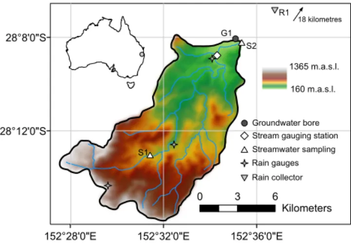
Figure 1. Upper Teviot Brook catchment and location of sam-pling sites. The stream gauging station corresponds to Teviot Brook at Croftby (145011A; operated by the Queensland Department of Natural Resources and Mines). The rainfall gauges correspond to Wilsons Peak Alert (040876), Carneys Creek The Ranch (040490) and Croftby Alert (040947), all run by the Bureau of Meteorology.
ii. Can short-term variations in older (5–100 years) groundwater contributions be captured by 3H
time-series data?
iii. How dissimilar are the RT of aquifers adjacent to streams (i.e. storage water) and the transit time of streamwater (i.e. exiting water)?
2 Study area 2.1 Physical setting
The upper Teviot Brook catchment is located south-west of Brisbane (south-eastern Queensland, Australia), with its headwaters in the Great Dividing Range (Fig. 1). It covers an area of 95 km2, and elevations range between 160 and 1375 m a.s.l.. Climate in the region is humid subtropical with
extremely variable rainfall: mean annual precipitation for the catchment is 970 mm (1994–2014 period), of which 76% falls from November to April. While Teviot Brook is a peren-nial stream, the distribution of discharge is uneven through-out the year: the mean annual discharge is 120 mm (1994– 2014 period), with highest and lowest streamflow occurring in February (average 40 mm) and September (average 2 mm), respectively. The headwaters support undisturbed subtropi-cal rainforest, while the valley supports open woodland and grassland.
val-ley is flatter and forms a wide alluvial plain. At this down-stream location the down-stream is incised into the alluvial de-posits, which at G1 are composed of fine-grained material, i.e. mostly gravel and silty clay. Underlying the alluvial de-posits is a sedimentary bedrock formation (Walloon Coal Measures) consisting of irregular beds of sandstone, silt-stone, shale and coal, some of which contain significant vol-umes of groundwater. Duvert et al. (2015b, a) reported high Fe concentrations and low3H activities for some
groundwa-ters of the sedimentary bedrock.
Hydraulic gradient analysis indicates that the alluvium mostly drains into the stream; hydrochemical and isotopic data also revealed a close connection between the alluvium and surface water in the Teviot Brook catchment (Duvert et al., 2015b). Borehole G1 is 13.9 m deep and it is screened from 12.3 m to its bottom, i.e. entirely within the alluvial stra-tum. The horizontal distance between G1 and S2 is 60 m.
2.2 Catchment hydrology
The monitoring period spans over 2 years, from mid-2012 to late 2014. Daily streamflow data were obtained from a gaug-ing station operated by the Queensland Department of Natu-ral Resources and Mines (Croftby station; 145011A) and lo-cated 2 km upstream of S2 (Fig. 1). Daily precipitation data were available at three rain gauges spread across the catch-ment and operated by the Australian Bureau of Meteorology. Average precipitation was calculated from the three records using the Thiessen method. Annual precipitation amounted to 1010 mm in 2012, 1190 mm in 2013 and 960 mm in 2014. The rainfall depths recorded in the headwaters were 100 to 250 mm higher than those in the floodplain. The maximum daily rainfall amount was 275 mm and occurred in late Jan-uary 2013, with a weekly value of 470 mm for this same event (Fig. 2a). This intense episode of rainfall generated a daily peak flow of 137 m3s−1 upstream of S2 (Fig. 3b),
which corresponds to a 22-year return period event at that station – calculated by fitting long-term data to a Galton dis-tribution. Earlier work has shown that this major event con-tributed significantly to recharge of the alluvial and bedrock aquifers in the headwaters (Duvert et al., 2015a, b). Another high flow event occurred in late March 2014, with a daily peak flow of 39 m3s−1. Generally, examination of the hydro-graph reveals that extended recession periods followed peak flows. Low flow conditions (Q <0.01 m3s−1) occurred
to-wards the end of the dry season, i.e. approximately from November through to January (Fig. 2b). The stream did not dry up during the study period although very low flow (Q <
0.001 m3s−1) occurred for 30 consecutive days in February–
March 2014.
3 Methods
3.1 Sample collection and analysis
Bulk samples of precipitation were collected at R1 (Fig. 1) at fortnightly to monthly intervals using a Palmex RS1 rainfall collector, which allows virtually evaporation-free sampling (Gröning et al., 2012). Streamwater and groundwater sam-ples were collected at S1 and S2 (stream sampling locations) and G1 (alluvial aquifer) following the same sampling de-sign as the rainfall samples. Samples at G1 were taken after measuring the water table level and purging a minimum of three casing volumes with a stainless steel submersible pump (Hurricane XL, Proactive). All samples were filtered through 0.45 µm membrane filters, and care was taken to seal the bot-tles and vials tightly to avoid evaporation.
Stable isotopes and chemical elements were measured for all samples at R1, S1, S2, and G1. 3H activity was
de-termined at S2 for most samples, and at G1 for one sam-ple. Chloride concentrations were measured using ion chro-matography (ICS-2100, Dionex), while iron and silicon were measured using inductively coupled plasma optical emission spectrometry (Optima 8300, Perkin Elmer). Total alkalinity was measured by titrating water samples with hydrochloric acid to a pH endpoint of 4.5. Major ions were assessed for accuracy by evaluating the charge balance error, which was
<10 % for all samples and<5 % for 93 % of the samples.
Samples were also analysed for 18O and 2H, using a Los
Gatos Research water isotope analyser (TIWA-45EP). All isotopic compositions in this study are expressed relative to the VSMOW standard (δ notation). Between-sample
mem-ory effects were minimised by pre-running all samples and subsequently re-measuring them with decreasing isotopic ra-tios, as recommended in Penna et al. (2012). Replicate anal-yses indicate that analytical error was±1.1 ‰ forδ2H and
±0.3 ‰ forδ18O. All these analyses were conducted at the
Queensland University of Technology (QUT) in Brisbane. In addition,3H was analysed at the Australian Nuclear Science and Technology Organisation (ANSTO) in Sydney. Samples were distilled and electrolytically enriched 68-fold prior to counting with a liquid scintillation counter for several weeks. The limit of quantification was 0.05 tritium units (TU) for all samples, and uncertainty was±0.06 TU. A sample collected in August 2013 was excluded from the data set since it was analysed twice and yielded inconsistent results.
3.2 Tracer-based calculation of transit and residence times
3.2.1 Using stable isotopes and chloride
com-0.001 0.01 0.1 1 10 100 0 100 200 300 P (m m ) Q (m 3s -1)
Jul-2013 Jan-2014 Jul-2014 Jul-2012 Jan-2013
Jul-2013 Jan-2014 Jul-2014 Jul-2012 Jan-2013
Jul-2013 Jan-2014 Jul-2014 Jul-2012 Jan-2013 Chloride Cl (m g/ L) Cl (m g/ L) 70 60 50 90 60 30 120 -5 -6.5 -3.5 -25 -35 -15 -1.5 -3 -4.5 -6 -10 -25 -40 -4.5 -4 -3.5 -20 -23 -26 -6 -4 -2 0 0 20 -20 -40 2H (‰ ) δ 18 O (‰ ) δ 18 O (‰ ) δ 18 O (‰ ) δ
(a)
(b)
(e)
(f)
δ 18O2H δ Cl (m g/ L) 12 10 8 14 0.5 1.5 2.5 3.5 Cl (m g/ L)
(c)
(d)
2H (‰ )δ 18
O (‰ ) δ 2H (‰ ) δ 2H (‰ ) δ
Figure 2.Time series of Thiessen-averaged precipitation(a), daily discharge at Croftby (DNRM station 145011A)(b), andδ2H,δ18O and chloride at R1 (rainfall)(c), S1(d)and S2 (streamwater)(e), and G1 (groundwater)(f). Note that theyaxes ofδ2H,δ18O and chloride have different scales for each individual plot.
position). An input recharge function was initially computed from the measured input data that accounts for loss due to evapotranspiration (e.g. Bergmann et al., 1986; Stewart and Thomas, 2008):
Cr(t )=R(t )
R (Cp(t )−Cr)+Cr, (1)
whereCr(t )is the weighted input recharge signature at time t;Cris the average recharge signature (taken at G1);Cp(t )is
the input rainfall signature;R(t )is the fortnightly recharge as
calculated by the difference between precipitation and evap-otranspiration; andRis the average recharge amount.
The weighted input was then convoluted to the selected TT distribution function (g) to obtain output signatures
(Mal-oszewski and Zuber, 1982):
Cout(t )= [g·Cr](t )= ∞
Z
0
Cr(t−te)g(te)e(−λte)dte, (2)
whereteis time of entry;Cout(t )is the output signature;Cr(t )
is the weighted input signature;g(te)is an appropriate TT
distribution function; ande(−λte)is the term that accounts for
decay if a radioactive tracer is used (λ=0 for stable isotopes and chloride). In this study we used both the exponential and dispersion models; the reader is referred to Maloszewski and Zuber (1982) and Stewart and McDonnell (1991) for a de-tailed overview of TT distribution functions.
be-Direct
runo
Older
component - TTD: go(te) - fraction:
y1
y2
o
Mountain front recharge
Stream at S1
Stream at S2 Younger component
- TTD: gy(te) - fraction: 1-
Subsurface /
shallow contribution
{
r1
r2
Diuse recharge
Deeper contribution
Storage water RTD: h(te)
{
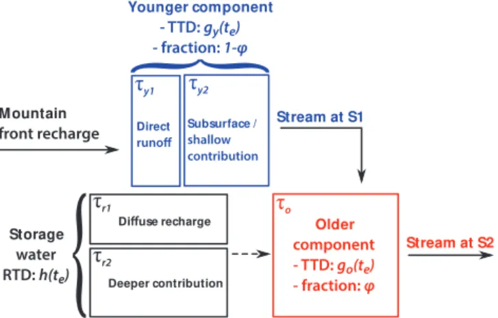
Figure 3.Conceptual diagram showing the flow components and
their transit times to be characterised in this study.
tween a shallower and a deeper flow component with shorter and longer TT, respectively. Bimodal models were obtained by linearly combining two TT distributions:
Cout(t )=φ
∞
Z
0
Cr(t−te)go(te)e(−λte)dte
+(1−φ)
∞
Z
0
Cr(t−te)gy(te)e(−λte)dte, (3)
whereφis the fraction of the older component (0< φ <1),
and go(te) and gy(te) are the TT distribution functions of
the older and younger components, respectively (Fig. 3). Bi-modal distributions combined either two dispersion models or one exponential and one dispersion model. The mean TTs, noted τ, were then derived from the fitted distributions by
calculating their first moment:
τ = ∞
Z
0
tg(t )dt. (4)
In the following the mean TT of the younger component is referred to asτy(subdivided intoτy1andτy2), while the mean
TT of the older component is referred to asτo, and the mean
RT of storage groundwater is referred to as τr (subdivided
intoτr1andτr2) (Fig. 3).
For chloride, the measured input and output series were highly dissimilar due to the significant effect of evaporative enrichment in soils. To get around this issue, a correction factor was applied to the predictions obtained using Eqs. (2) and (3):Cout(t )values were multiplied byF =(P−PET) (i.e. ratio between precipitation and recharge over the preceding 12 months). The reasoning behind the use of this correction factor was that all chloride ions find their way through the soil, whereas much of the rainfall is evaporated off.
To estimate the fraction of older water that contributed to streamflow, a simple two-component hydrograph separation
was carried out (Sklash and Farvolden, 1979) based on fort-nightly data of each of the three seasonal tracers. This al-lowed one to obtain time-varying values ofφ:
φ (t )=δS1(t )−δR1(t )
δG1−δR1(t ) , (5)
whereδS1,δR1 andδG1 are the tracer values of streamflow,
rainfall and groundwater, respectively. The use of a chemi-cal mass balance approach to partition streamflow was pre-ferred over recursive digital filtering (Nathan and McMahon, 1990), because the former method is less likely to include delayed sources, such as bank return flow and/or interflow, in the older water component (Cartwright et al., 2014).
3.2.2 Using tritium
The occurrence of seasonal variations in rainfall3H
concen-trations has been widely documented (e.g. Stewart and Tay-lor, 1981; Tadros et al., 2014). These variations can be sig-nificant and have to be considered for achieving reliable es-timates of TT distributions. Monthly3H precipitation data
measured by ANSTO from bulk samples collected at Bris-bane Aero were used to estimate the3H input function for
the Teviot Brook catchment. Because Brisbane Aero is ca. 100 km north-east of Teviot Brook, the rainfall3H concen-trations are likely to be significantly different between these two locations due to oceanic and altitudinal effects. Accord-ing to Tadros et al. (2014),3H values for Toowoomba (i.e.
lo-cated in the Great Dividing Range near Teviot Brook) were about 0.4 TU above those for Brisbane Aero for the period 2005–2011. Based on this work, an increment of+0.4 TU was applied to values measured at Brisbane Aero in order to obtain a first estimate of rainfall 3H concentrations for
Teviot Brook (input series A2 in Table 1). A second estimate was obtained by comparing the historical3H data between
Toowoomba and Brisbane Aero for the period with overlap between the two stations, i.e. 1968–1982. All monthly val-ues with precipitation>100 mm, corresponding to rainfall
likely contributing to recharge, were included in the analy-sis (n=31). A scaling factor of 1.24 was derived from the correlation between the two stations (R2=0.80). This factor
was used to compute input series B2 (Table 1).
To account for losses due to evapotranspiration as rain-fall infiltrates into the ground, a weighting procedure similar to the one reported by Stewart et al. (2007) was developed. Monthly3H recharge was estimated by subtracting monthly
evapotranspiration from monthly precipitation, and weight-ing the3H rainfall concentrations by the resulting recharge.
Instead of calculating single annual values, 6-month and 1 yr sliding windows were used to obtain monthly values as fol-lows:
Ci= Pi
i−tCjrj Pi
i−trj
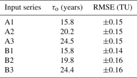
Table 1.Description of the different3H input series computed for the Teviot Brook catchment.
Input series Description of input parameters
A1 A2−25 %
A2 Brisbane Aero3H values+0.4 TU
A3 A2+25 %
B1 B2−90 % CI slope
B2 Brisbane Aero3H values×1.24 TU
B3 B2+90 % CI slope
CI refers to the confidence interval on the Toowoomba vs. Brisbane Aero regression slope.
where Ci is the monthly 3H recharge for the ith month, Cj and rj are the monthly 3H precipitation and monthly
recharge rate for thejth month, andtis 6 or 12 depending on
the span of the sliding interval used. To avoid edge effects, a Tukey filter (Tukey, 1968) with coefficient 0.6 was applied to the sliding windows.
Input (recharge) and output (streamwater)3H
concentra-tions were then related using the same convolution integral as the one used for stable isotopes (Eqs. 2 and 3), withλthe 3H decay constant such thatλ=1.54×10⁻⁴day−1. To ac-count for the uncertainty in input parameters and to assess the sensitivity of TT distribution calculations to the input func-tion, four additional input series were derived from A2 and B2 (Table 1), and all six input series were subsequently used in the calculations. Least square regressions were used, and root mean square errors (RMSE) were calculated to find the best data fit for each simulation using a trial and error pro-cess. All data processing and analyses were performed using Matlab version 8.4.0 (R2014b), with the Statistics toolbox version 9.1.
4 Results
4.1 Seasonal tracers in precipitation, streamwater and groundwater
4.1.1 Description
Stable isotope ratios and chloride signatures in precipitation were highly variable throughout the study period (Figs. 2c and 4). The δ2H and δ18O rainfall values ranged between
−41 and +12 ‰ (average−12 ‰) and between −6.5 and
−0.1 ‰ (average−3.1 ‰), respectively, while chloride
con-centrations ranged between 0.6 and 3.2 mg L−1 (average 1.8 mg L−1). Generally, the most significant rainfall events
had isotopically depleted signatures. As an example, there was a considerable drop in all tracers during the January 2013 event (e.g. forδ2H: decrease from−16 to−41 ‰; Fig. 2c).
The local meteoric water line derived from rainfall samples had an intercept of 15.8 and a slope of 8.4 (Duvert et al., 2015b), similar to that of Brisbane (Fig. 4a). The stable
iso-tope ratios measured in streamwater at S1 (Fig. 2d) and S2 (Fig. 2e) also covered a wide range of values, and followed similar temporal patterns to those for rainfall. However, the overall variations were less pronounced in streamwater, with evident dampening of input signals. Average values were lower for S1 (δ2H= −25 and δ18O= −4.9 ‰) than for
S2 (δ2H= −20 andδ18O= −3.7 ‰), both locations having
lower average values than rainfall. All S1 samples aligned close to the meteoric water line, whereas most S2 samples plotted along a linear trend to the right of the line (Fig. 4a). Chloride concentrations in streamwater ranged between 6.4 and 12.8 mg L−1at S1, and between 35.1 and 111.1 mg L−1 at S2 (Figs. 2d and e, 4b). At S2, higher chloride values were consistent with higherδ18O values andvice versa, whereas there was a weaker correlation between the two tracers at S1 (Fig. 4b). The fluctuations in stable isotopes and chlo-ride in groundwater were considerably attenuated as com-pared to rain and streamwater (Figs. 2f and 4). The δ2H, δ18O and chloride values recorded at G1 tended to slightly
decrease during the rainy season, although they stayed within the ranges−22±3,−3.9±0.4 ‰ and 60±10 mg L−1, re-spectively (Fig. 2f). Consistent displacement to the right of the meteoric line was observed for all G1 samples (Fig. 4a).
4.1.2 Interpretation
The large temporal variability observed in rainfall isotopic and chloride records (Fig. 2c) may be attributed to a com-bination of factors. First, there was an apparent seasonal cy-cle as values were higher in the dry season and tended to decrease during the wet season. These are well-known fea-tures for rainfall that can be related to the “amount effect” (Dansgaard, 1964) where raindrops during drier periods ex-perience partial evaporation below the cloud base, typical in tropical to subtropical areas (Rozanski et al., 1993). Sec-ond, more abrupt depletions of 2H and 18O occurred
observa--6 -5 -4 -3 -2 -35
-30 -25 -20 -15 -10
-6 -5 -4 -3 -2
0 20 40 60 80 100 120
-6 -3 0
-40 -20 0
2
H (‰
)
δ
18
O (‰)
δ
Cl (m
g/L)
(A)
(B)
S2 G1 S1 R1
LMW L
Figure 4.Relationships between(a)δ2H andδ18O and(b)chloride
and δ18O for rainfall, streamwater and groundwater of the Teviot Brook catchment. The local meteoric water line plotted in(a)
fol-lows the equationδ2H=8.4·δ18O+15.8 (Duvert et al., 2015b). The eight R1 samples withδ18O values either<−6.2 ‰ or>−1.5 ‰ are not shown in(b); chloride concentrations for these samples were in the range 0.6–3 mg L−1.
tion in Australian catchments, largely attributed to high rates of evapotranspiration that concentrate cyclic salts in the un-saturated zone, thereby increasing the salinity of subsurface water before it discharges into streams (e.g. Allison et al., 1990; Cartwright et al., 2004; Bennetts et al., 2006).
4.2 Tritium in precipitation, streamwater and groundwater
4.2.1 Description
The groundwater sample collected at G1 in October 2012 yielded a3H activity of 1.07±0.06 TU. Additional data was
obtained from Please et al. (1997), who collected a sample at the same location in 1994. This earlier sample had an activity of 1.80±0.20 TU. The 20 samples of streamwater collected
Table 2.Kendall’sτ and Pearson’sr correlation coefficients be-tween3H and other variables at S2.
Variable r τ
Mean daily discharge (m3s−1) 0.47 0.06
δ2H (‰) −0.27 −0.06
δ18O (‰) −0.23 0.02
Cl (mg L−1) −0.12 0.03
Si (mg L−1) 0.35 0.11
Alkalinity (mg L−1) −0.32 −0.13
Fe (mg L−1) 0.25 0.11
AntecedentP in the last 15 days (mm) 0.32 −0.01
Last day withP >2 mm (–) 0.11 0.03
No value was statistically significant atp <0.05 for both tests.
at S2 showed variable3H activities ranging between 1.16±
0.06 and 1.43±0.06 TU (Fig. 5).
In order to estimate a3H input signal for the Teviot Brook
catchment, several precipitation time series were calculated from Brisbane Aero monthly3H data set, as detailed in
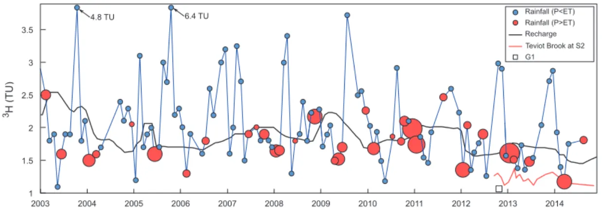
Ta-ble 1. Recharge time series were then derived from these precipitation time series using Eq. (6). An example of the calculated monthly precipitation and recharge time series for the 2003–2014 period is presented in Fig. 6 for scenario A2. While the 3H activity in rainfall ranged between 1.1 and
6.4 TU for A2, most of the rainfall events contributing to recharge (i.e. for which monthly precipitation prevailed over monthly evapotranspiration; red circles in Fig. 6) remained in the narrower range 1.5–2.5 TU.
4.2.2 Interpretation
The 3H activity in rainfall showed considerable
month-to-month variability. Winter (dry season) values generally were higher than summer (wet season) values, consistent with re-sults from Tadros et al. (2014). Among the 203H values
ob-tained at S2, higher values tended to coincide with higher flow conditions, although it was not systematic (Fig. 5). For instance, the sample collected in January 2013 under low flow conditions yielded 1.35±0.06 TU; by contrast, the
sam-ple collected in April 2014 during the falling limb of a major runoff event yielded 1.19±0.06 TU, i.e. among the lowest
values on record. Kendall’s rank correlation and Pearson’s coefficients were calculated between the3H measurements
in streamwater and other hydrological, hydrochemical and isotopic variables (Table 2).3H activity was not significantly
correlated with any of the other variables. Unlike in Morgen-stern et al. (2010) and Cartwright and MorgenMorgen-stern (2015), there was no strong linear relationship between flow rate and
3H activity in the stream. The lack of strong correlation
be-tween3H and variables such as antecedent wetness
Q
(m
3s -1)
3H
(T
U
)
Q
(m
3s -1)
Jan-12 Jul-12 Jan-13 Jul-13 Jan-14 Jul-14
100
1
0.01
1.1 1.2 1.3 1.4
1
0.1
0.01
0.001 10 100
20 40 60 80 100
0
Exceedance (%)
Figure 5.Time series of3H activity at S2 and daily discharge data (left). Flow duration curve at S2 (right). The six red circles correspond to
samples used to fit the low baseflow model (see Fig. 9). The whiskers correspond to measurement uncertainty (±0.06 TU for all samples).
1 1.5 2 2.5 3 3.5
2003 2004 2005 2006 2007 2008 2009 2010 2011 2012 2013 2014
3H
(T
U
)
Rainfall (P<ET)
Recharge Teviot Brook at S2 Rainfall (P>ET)
G1
4.8 TU 6.4 TU
Figure 6.Temporal evolution of input3H in precipitation (circles) and recharge (black line) for the Teviot Brook catchment considering the A2 scenario. The plotted circles correspond to rainfall collected at Brisbane Aero and adjusted to Teviot Brook according to A2. The recharge time series was obtained using Eq. (6) and a 12-month sliding window. The marker size for rainfall contributing to recharge (red circles) reflects the recharge rate.
4.3 Residence time estimate for storage water
The sample collected at G1 in October 2012 (3H=1.07±
0.06 TU) suggests that alluvial groundwater contains a
sub-stantial modern component, because its 3H concentration
was only slightly below that of modern rainfall. An earlier
3H value reported by Please et al. (1997) was re-interpreted
and combined with our more recent measurement to pro-vide additional constraints on the RT at G1. Two steady-state models were adjusted to the data points. The first model to be tested was a unimodal dispersion model while the second one was a bimodal exponential–dispersion model. For the bi-modal model, the mean RT of younger componentsτr1 was
constrained to 1 year, and the fraction of younger water was constrained to 57 % as these parameters provided best fits on average.
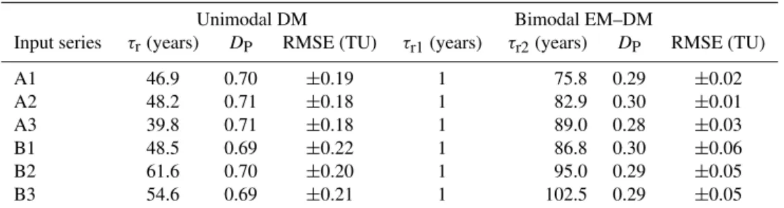
Results for both models are presented in Table 3 and the two fits using A2 as an input function are shown in Fig. 7. As expected, mean RTs varied as a function of the input function chosen: values were generally lowest with A1 and B1 and highest with B3. Both models provided reasonably good fits, although for all simulations the bimodal
distribu-tion described more accurately the measured data (median RMSE 0.04 vs. 0.20 TU; Table 3). Unimodal distributions hadτr ranging between 40 (using A3 as input series) and
62 years (using B2 as input series), with a standard deviation of 7 years among all simulations. The older water fraction of bimodal models hadτr2between 76 (using A1 as input
se-ries) and 102 years (using B3 as input sese-ries), with a standard deviation of 9 years.
4.4 Transit time estimates using seasonal tracers Lumped parameter models were adjusted to the stable iso-tope and chloride time series at S1. Due to the limited number of fortnightly data, all values were included in the analysis, i.e. samples collected under both low baseflow and higher flow conditions. Two models were tested and compared for this purpose, a unimodal exponential model and a bimodal exponential–dispersion model (Table 4; Fig. 8).
Table 3.Results of model simulations of residence time for G1 using3H.
Unimodal DM Bimodal EM–DM
Input series τr(years) DP RMSE (TU) τr1(years) τr2(years) DP RMSE (TU)
A1 46.9 0.70 ±0.19 1 75.8 0.29 ±0.02
A2 48.2 0.71 ±0.18 1 82.9 0.30 ±0.01
A3 39.8 0.71 ±0.18 1 89.0 0.28 ±0.03
B1 48.5 0.69 ±0.22 1 86.8 0.30 ±0.06
B2 61.6 0.70 ±0.20 1 95.0 0.29 ±0.05
B3 54.6 0.69 ±0.21 1 102.5 0.29 ±0.05
DM stands for dispersion model; EM–DM stands for exponential–dispersion model;DPstands for dispersion parameter. For the EM–DM,τr1was constrained to 1 year, and the fraction of younger water was constrained to 57 %.
1 1.5 2 2.5
1990 1995 2000 2005 2010 2015
Measurements
Model 1 (unimodal)
Model 2 (bimodal)
3 H
a
t
G
1
(T
U
)
Figure 7. Fits of two models at G1 using A2 as input 3H
se-ries. The unimodal model is a dispersion model with first moment 48.2 years and dispersion parameter 0.71. The bimodal model is an exponential–dispersion model: a younger component (exponen-tial distribution; fraction 57 %) with first moment 1 year and an older component (dispersion distribution; fraction 43%) with first moment 82.9 years and dispersion parameter 0.30. The 1994 mea-surement is from Please et al. (1997).
lines in Fig. 8). All three tracers yielded comparable expo-nential TT distribution functions, withτyranging between 65
and 70 days (Table 4). The bimodal models provided slightly more satisfactory fits for all tracers (black lines in Fig. 8), with lower RMSE overall. Bimodal TT distribution functions derived from data at S1 had a younger fraction (27 %) with
τy1 between 14 and 16 days, and an older fraction (73 %)
withτy2 between 113 and 146 days (Table 4) depending on
which tracer was used.
Calibration was also carried out on the tracer time series collected at S2 and following the same procedure (Table 4). When considering a unimodal exponential distribution, all three tracers yielded comparable TT distribution functions, withτyranging between 71 and 85 days, which was slightly
longer than the mean TTs calculated at S1. When considering a bimodal exponential–dispersion distribution, the younger fraction hadτy1of 23 to 24 days, while the older fraction had τy2of 99 to 109 days (Table 4).
4.5 Transit time estimates using tritium
4.5.1 Model adjustment to low baseflow samples A lumped parameter model was fitted to the six 3H
sam-ples that were taken under low baseflow conditions, i.e.Q <
0.01 m3s−1. The model chosen for this purpose was a
bi-modal exponential–dispersion model; the fitting procedure was as follows:
– The dispersion parameter of the older component was loosely constrained to around 0.3 in order to mimic the shape of the TT distribution identified at G1 (Sect. 4.3). The old water fractionφ was constrained to 82 %, i.e.
the average value obtained for the six baseflow sam-ples using tracer-based hydrograph separation following Eq. (5).
– Initial simulations were run using the six input series with no further model constraint. For the six scenarios,
τyconsistently converged to 0.33±0.08 years.
– All models were then re-run while adding the additional constraint as noted above, so that the only parameter to be determined by fitting wasτo.
Figure 9 provides an example of the adjustment using A2 as input3H function. Reasonably good fits were obtained for all simulations (0.14 TU<RMSE<0.16 TU), with τo
be-tween 15.8 and 24.5 years, average 20.1±3.9 years (Table 5).
4.5.2 Model adjustment to single tritium values Unlike for rainfall3H values where high temporal
variabil-ity was observed, the derived time series for recharge was relatively constant over the last decade (Fig. 6). This charac-teristic in principle allows reliable assessment of catchment TTs with single3H measurements, providing the3H
(days)
50 100 150
R
MS
E
0.3 0.35
0.4 10 20 30 40
(d
a
ys)
10 20 30 40
y20.6 0.8
(days)
(d
a
ys)
80 120 160 200
0.28 0.333 0.39
10 20 30 40
(d
a
ys)
80 120 160 200
0.1 0.20
0.15
80 120 160
200 1
(a)
(d)
(g)
(b)
(e)
(h) (i)
(f) (c)
y28 10 12 14
6
50 100 150
R
MS
E
0.05 0.15 0.25
50 100 150
R
MS
E
0.6 8
1 1.4 Oct-12 Jan-13 Apr-13 Jul-13 Oct-13 Jan-14 Apr-14
1
8
-6 -5 -4 -3
Oct-12 Jan-13 Apr-13 Jul-13 Oct-13 Jan-14 Apr-14
2
-35 -30 -25 -20 -15
Oct-12 Jan-13 Apr-13 Jul-13 Oct-13 Jan-14 Apr-14
C
l
(mg
/L
)
Measurements Unimodal Bimodal
y1 y2 yFigure 8.Exponential (blue) and exponential–dispersion (black) models calibrated to theδ18O(a),δ2H(d)and chloride(g)time series at S1.
Whiskers correspond to the measurement uncertainty as given in the Methods section. Root mean square errors (RMSEs) of the exponential model as a function ofτyfor the three tracers(b, e, h). RMSE of the exponential–dispersion model (27 % younger component; dispersion parameter 0.3) as a function of mean transit times of the younger (τy1) and older (τy2) fractions for the three tracers (c,fandi). Lighter
colours are for lower RMSE, and the smallest contours correspond to the range of acceptable fit, arbitrarily defined as the values for which the RMSE are lower than the lowest RMSE obtained with the exponential models. Results for these simulations are reported in Table 4.
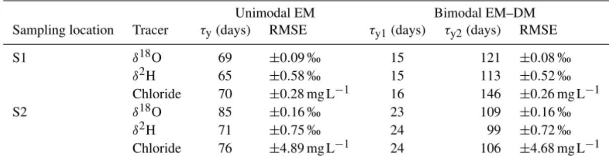
Table 4.Results of model simulations of transit time for S1 and S2 usingδ2H,δ18O and chloride.
Unimodal EM Bimodal EM–DM
Sampling location Tracer τy(days) RMSE τy1(days) τy2(days) RMSE
S1 δ18O 69 ±0.09 ‰ 15 121 ±0.08 ‰
δ2H 65 ±0.58 ‰ 15 113 ±0.52 ‰
Chloride 70 ±0.28 mg L−1 16 146 ±0.26 mg L−1
S2 δ18O 85 ±0.16 ‰ 23 109 ±0.16 ‰
δ2H 71 ±0.75 ‰ 24 99 ±0.72 ‰
Chloride 76 ±4.89 mg L−1 24 106 ±4.68 mg L−1
EM stands for exponential model; EM–DM stands for exponential–dispersion model. For the EM–DM, the dispersion parameter of the second mode was 0.3 and the fraction of younger water was 27 %.
the TT of the old water fraction (τo). The model parameters
were chosen according to the best fit obtained for baseflow samples (i.e. mean TT of young component τy 0.33 years,
dispersion parameter of old component 0.3; Sect. 4.5.1). In addition, for each sample the fraction of old water φ was
constrained to the value obtained using tracer-based hydro-graph separation according to Eq. (5). Conceptually, this ap-proach appeared more meaningful than another option that would have consisted in constraining τo and subsequently
determining the old water fractionsφ, because there was no
indication thatτoremained constant over time. Simulations
were carried out for all three hydrograph separation tracers and all six input series, and the sensitivity of simulations to both the3H measurement uncertainty (±0.06 TU) and the er-ror related to the hydrograph separation procedure were also calculated.
Time series of τo were derived for each input function,
and Fig. 10 shows the results obtained with A2 as an in-put series. The old water fractionφvaried between 0.39 and
1 1.4 1.8 2.2
2002 2004 2006 2008 2010 2012 2014
1.2 1.3
2013 2014
Exponential (0.18) + Dispersion (0.82) model EM:
DM:
Baseflow
(Q < 0.01 m3s-1)y= 0.33 year
= 20.2 years; PD= 0.3
o
3
H
a
t
S
2
(T
U
)
Figure 9.Bimodal model fitted to the3H activities at S2 under low
baseflow conditions (i.e. dailyQ <0.01 m3s−1). A2 was used as input3H series for this case. Results using other input series are listed in Table 5.
Table 5.Results of model simulations of transit time for S2 under low baseflow conditions (i.e. dailyQ <0.01 m3s−1), using3H and an exponential–dispersion model.
Input series τo(years) RMSE (TU)
A1 15.8 ±0.15
A2 20.2 ±0.15
A3 24.5 ±0.15
B1 15.8 ±0.14
B2 19.8 ±0.16
B3 24.4 ±0.16
The mean TT of younger components (τy) was constrained to 0.33 years, the dispersion parameter of older components was constrained to 0.3, and the ratio of older water was constrained to 82 %.
tracers, hydrograph separation based on chloride generally yielded lower variations in φ over time (Fig. 10a).
Gener-ally, the older component was lowest during high flow con-ditions and greatest during recession periods. The simulated
τo values varied considerably over time, and variations
ex-ceeded the uncertainties related to measurement uncertain-ties, chemical mass balance calculation errors and input esti-mates (Fig. 10b–d).18O was the least accurate in evaluating the variations in τo (wider range for the red shaded area in
Fig. 10c), while chloride was the most accurate despite less pronouncedτovariations (narrower range for the red shaded
area in Fig. 10d). Yet, all three tracers provided comparable results, with a consistent shift in values either upwards or downwards. As a general rule, there was a negative correla-tion betweenφandτo. When using A2 as input function,τo
fluctuated between 11.9 and 58.0 years (2H; Fig. 10b), 11.6
and 63.2 years (18O; Fig. 10c) and 11.5 and 42.1 years
(chlo-ride; Fig. 10d). For clarity purposes theτovalues reported in
the text do not consider errors related to measurement uncer-tainty. Values were highest after the major recharge events
that occurred in January and February 2013, withτobetween
26.8 and 63.2 years in late February, and in April 2014, with
τo between 28.3 and 55.1 years. They were lowest during
periods undergoing sustained low flow such as in Septem-ber 2012 (τobetween 11.6 years for18O and 13.1 years for 2H) and in September 2013 (τ
obetween 11.5 years for
chlo-ride and 11.9 years for2H). Of note is the timing of the
high-estτovalue in late February 2013, i.e. 1 month after the major
recharge episode.
5 Discussion
5.1 Conceptual framework
According to our conceptual understanding of the upper Teviot Brook catchment, we have partitioned streamflow into two major components (Fig. 3). The first end-member represents the contribution of younger waters from rapid recharge through the highly fractured igneous rocks form-ing the mountain front, as outlined in previous studies (Du-vert et al., 2015b, a). This younger component was further divided into (i) quick flow and (ii) relatively delayed contri-bution of waters seeping from the rock fractures (Fig. 3). We assume that the TTs of the younger end-member can be ac-curately described through analysis of the seasonal tracers’ signal dampening. Waters originating from this component typically had low total dissolved solid (TDS) concentrations, although high Si concentrations at high flow.
The second end-member we postulate contains older wa-ters derived from the aquifer stores located in the lowland section of the study area (Fig. 3). Specifically, these are wa-ters discharging from both the alluvial aquifer and the un-derlying sedimentary bedrock aquifer. Although a distinc-tion between the two groundwater stores would be ideal, the lack of clear differentiation between both water types led us to consider one single “older water” component. We as-sume that the TTs of the older end-member may be accu-rately described through3H data analysis. The3H activities
in both aquifers were generally lower than those in surface water; the sedimentary bedrock aquifer had on average lower
3H values than the alluvial aquifer, and waters from both
aquifers had varying but generally high TDS concentrations (Duvert et al., 2015b). Furthermore, higher Fe concentrations were observed in the sedimentary bedrock waters shortly af-ter recharge (Duvert et al., 2015a).
In the next sections of the discussion, a stepwise approach is followed to evaluate the accuracy of the conceptual model outlined above. In particular, the younger and older compo-nents in streamflow are assessed and discussed in Sect. 5.2 and 5.3, respectively. Section 5.4 considers the relationships between the older streamflow component and groundwater stored in the catchment. The variations over time of the TTs of the older componentτoare then quantified and elucidated
10 20 40 60
10 20 40 60
Oct-12 Jan-13 Apr-13 Jul-13 Oct-13 Jan-14 Apr-14 Jul-14 Oct-14
(years)
10 20 40 60
Oct-12 Jan-13 Apr-13 Jul-13 Oct-13 Jan-14 Apr-14 Jul-14 Oct-14
φ
(-)
(a)
(b)
(c)
(d)
0.40.6 0.8 1
τ
o(years)
τ
o(years)
τ
oOxygen-18 Deuterium Chloride
100 100 100
Figure 10.Variations in the older component fractionφaccording to the three seasonal tracers (using Eq. (5))(a). Variations in the TT of
older fractionτoat S2 based on hydrograph separation using2H(b),18O(c)and chloride(d). Values in(b–d)were obtained through the adjustment of exponential–dispersion models to each3H sample separately, and using A2 as input series and a 12-month sliding window. Whiskers represent the error range due to the measurement uncertainty on each sample (i.e.±0.06 TU). The blue shaded areas represent
the range of values due to uncertainties in the estimation of recharge input (i.e. for the six3H input time series), while the red shaded areas represent the range of error related to the calculation ofφ, which was estimated according to the method described in Genereux (1998) and propagated to the calculation ofτo.
current methodology and raises new questions for future re-search.
5.2 Identification of a younger component in streamflow
The younger end-member was defined by adjusting lumped models to the seasonal tracer time series (Sect. 4.4; Fig. 8). Among all the TT distributions described in the literature, the exponential model was selected because it considers all possible flowpaths to the stream – the shortest flowpath hav-ing a TT equal to zero and the longest havhav-ing a TT equal to infinity (e.g. Stewart et al., 2010). Importantly, this distri-bution assumes heavy weighting of short flowpaths, which in our case may accurately replicate the prompt response of streamflow to rainfall inputs in the headwaters.
At S1, the bimodal distribution provided the most accurate simulations (Table 4), which lends support to the occurrence
of two end-members contributing to streamflow at this up-stream location. The first (exponential) component may re-flect quick flow and subsurface waters feeding the stream (τy1between 14 and 16 days), while the second (dispersion)
component may be attributed to the contribution of waters discharging from the highly fractured igneous rocks (τy2
be-tween 113 and 146 days; Fig. 8). Results at S2 were also slightly more accurate when using a bimodal distribution, suggesting a dual contribution to streamflow at S2 as well. More importantly, the fits for S2 were not as accurate as those for S1, regardless of the distribution and tracer used (Table 4). This reflects the likely importance of other concur-rent processes in the downstream section of the catchment. Among them, evaporation may be a major limitation to ap-plying steady-state lumped models at S2. It has been reported that18O is generally more sensitive to the effects of
2015b). However, in this study there were no significant dif-ferences between TT distributions derived from the two sta-ble isotopes. Calibration of the models on chloride measure-ments did not yield as accurate results as those for stable isotopes at S1 and to a higher extent at S2, which may be attributed to the higher effects of evaporative enrichment on chloride. Based on flux tracking methods, Hrachowitz et al. (2013) showed that processes such as evaporation can result in considerable biases in TT distribution estimates when us-ing chloride as a tracer.
It is increasingly recognised that stable isotopes cannot provide realistic estimates of longer TT waters, regardless of the lumped model used (Stewart et al., 2012; Seeger and Weiler, 2014; Kirchner, 2015). In this study, it is very likely that older water (i.e. >5 years) contributed to streamflow
at S2 (see Sect. 5.3) but also possibly at S1, and only us-ing stable isotopes and chloride does not allow detection of such contribution. Therefore the ages defined above should be regarded as partial TTs that reflect the short-term and/or intermediate portions of the overall TT distribution for the system, i.e.τyrather thanτ (Seeger and Weiler, 2014).
5.3 Identification of an older component in streamflow The transfer function that provided the most accurate es-timates of TT for the baseflow samples at S2 was an exponential–dispersion model (Sect. 4.5.1). While other dis-tributions could have been tested, there is a large body of literature that has reported good agreement between expo-nential, exponential-piston flow and dispersion models cal-ibrated to 3H data (e.g. Maloszewski et al., 1992;
Her-rmann et al., 1999; Stewart et al., 2007; Cartwright and Morgenstern, 2015). The good fits obtained using this bi-modal function (Fig. 9; Table 5) confirm that two major wa-ter sources contributed to streamflow at S2. It can be argued that the exponential component captured all young contribu-tions from upstream, i.e. quick flow + soil water + discharge from fractured igneous rocks, as identified in Sect. 5.2 (τy= 0.33 years), while the dispersion component encompassed
the delayed groundwater flowpaths (τo between 15.8 and
24.5 years). This older contribution to streamflow may orig-inate from the alluvial aquifer, potentially supplemented by seepage from the bedrock storage, as discussed in Sect. 5.1.
A number of studies were carried out in the last 4 decades that also used3H to assess TTs of the baseflow component
to streams. For catchment areas in the range 10–200 km2,
TT estimates were between 3 and 157 years (n=39; me-dian 12 years; data presented in Stewart et al. (2010) supple-mented with later papers by Morgenstern et al. (2010), Kralik et al. (2014) and Cartwright and Morgenstern (2015)). While our results compare relatively well to the literature, estimates can vary greatly even within single catchments (e.g. Morgen-stern et al., 2010). Also, all reported studies were conducted in temperate regions, this work being the first one carried out in a subtropical setting.
5.4 Storage water and its relationships with the older streamflow component
Simulations of groundwater RT using3H as a tracer are
gen-erally insensitive to the type of lumped parameter model cho-sen, given that ambient 3H levels are now almost at
pre-bomb levels (e.g. Stewart and Thomas, 2008). At G1, bet-ter fits were obtained for bimodal functions (Fig. 7; Ta-ble 3). This may be interpreted as the probaTa-ble partitioning of groundwater into one contribution of younger waters by diffuse recharge or flood-derived recharge (τr1≈1 year) cou-pled with a second contribution of older waters, potentially seeping from the underlying sedimentary bedrock aquifer (τr2≈80 to 100 years).
While the older component to streamflow as identified in Sect. 5.3 was characterised by relatively old waters with TT in the range 15.8–24.5 years, this contribution could not be directly related to the RT of storage waters (i.e. τo6=τr).
Despite the exclusive use of samples taken under low base-flow conditions to determine τo, the obtained values were
significantly lower than the estimates of τr2 for the
allu-vial aquifer (average 20.1±3.9 vs. 88.7±9.3 years,
respec-tively). This confirms that water stored in the catchment (res-ident water) and water exiting the catchment (transit wa-ter) are fundamentally different and do not necessarily fol-low the same variations, as recognised in recent work (e.g. Hrachowitz et al., 2013; van der Velde et al., 2015). Re-sults from a dynamic model of chloride transport revealed that water in transit was generally younger than storage wa-ter (Benettin et al., 2015). Differences between RTs and TTs also indicate that the assumption of complete mixing was not met for the Teviot Brook catchment. This corroborates the findings from van der Velde et al. (2015), who established that complete mixing scenarios resulted in incorrect TT es-timates for a catchment subjected to high seasonal rainfall variability. For instance, shallow flowpaths may be activated or deactivated under varying storage. Among the few stud-ies that investigated the relations between catchment TT and groundwater RT based on3H measurements, Matsutani et al. (1993) reported that streamwater was formed by a mixture of longer RT groundwater (19 years) and shorter RT soil water (<1 year). Overall, more work is needed to better define the
two distributions and to assess how they relate to each other under non-stationary storage conditions.
5.5 Drivers of the variability in the older component transit time
When fitting models to each 3H value in streamwater, τ o
was found to vary substantially over time (Fig. 10). In or-der to better apprehend the factors influencing the varia-tions inτo, the obtained values were compared to other
conditions (P15<5 mm), there was no consistent
relation-ship betweenτo and the amount of precipitation during the
15 days prior to sampling, withτoranging between 14.9 and
23.1 years (n=3; Fig. 11a). For higher values of P15 (i.e. P15≥10 mm), there was a positive correlation between the two variables (n=17,R2for power law fit = 0.47, p-value
= 0.002). The TT of the old water fraction was lowest for
P15 between 10 and 50 mm (τo 11.9 to 25.5 years), and it
increased when antecedent precipitation increased (τo 25.6
to 58.0 years forP15>100 mm). Generally, values averaged
17.0±5.6 years at low flow and 38.3±14.7 years after major
high flow events. This was in accordance with results from Fig. 10, and suggestive of the predominant contribution of older alluvial and/or bedrock waters shortly after recharge episodes.
There was also a positive relationship betweenτoand Fe
concentrations at S2 (n=20,R2for power law fit=0.48,
p-value=0.001), with all the values>0.2 mg L−1 correspond-ing to τo>30 years (Fig. 11b). In contrast, no significant
relationship was observed at S1, as Fe values at this sta-tion ranged between<0.01 and 0.96 mg L−1. Duvert et al.
(2015a) reported increasing Fe concentrations after a ma-jor recharge event for some groundwaters of the sedimen-tary bedrock. The increase in streamflow Fe might there-fore be a result of enhanced discharge of these waters into the drainage network, which is coherent with older τo
val-ues. However, other chemical parameters distinctive of the bedrock groundwaters did not produce a characteristic sig-nature in streamflow during high flow conditions. Or else, high Fe concentrations may be simply due to higher weath-ering rates at higher flows, although this hypothesis disre-gards the high value measured for the April 2014 sample (Fe=4.15 mg L−1) despite relatively low discharge (Q= 0.095 m3s−1).
As discussed previously, a modification in storage due to a change in recharge dynamics may have activated differ-ent groundwater flowpaths and hence water parcels with dif-ferent RTs (Heidbüchel et al., 2013; van der Velde et al., 2015; Cartwright and Morgenstern, 2015). When the rate of recharge was highest, flushing out of waters located in the deeper, older bedrock aquifer may have been triggered by the resulting pressure wave propagation. By contrast, the rela-tively youngerτoobserved during lower flow conditions may
be attributed to waters that originate from shallower parts of the alluvium and/or from subsurface layers. This is reflected in the relationship between τo and Qo, i.e. the portion of
streamflow provided by the older component (Qo=Q·φ;
Fig. 11c). In this figure the groundwater end-member cor-responds to τr (using the highest recorded Qo through the
study period), while the baseflow end-member corresponds to the τo value calculated using the six baseflow samples.
The two end-members were linearly connected in an area that represents the extent of possible fluctuations ofτo, from
lower old water contributions to higher old water contribu-tions. The individualτovalues broadly followed this mixing
P
15(mm)
10-1 100 101 102 103
10 20 30 50 70
10-2 10-1 100 101
10 20 30 50 70
10-3 10-2 10-1 100
10 100
20 50
Fe (mg L-1)
(ye
a
rs)
o(ye
a
rs)
o(a)
(b)
Qo = 2 m3s-1Qo = 2 10-3 m3s-1
(ye
a
rs)
oQo (m3 s-1) Baseflow end-member Groundwater end-member
(c)
Figure 11.Relationship between the transit time of old water frac-tion (τo) and antecedent precipitationP15, i.e. precipitation depth over the catchment during the 15 days prior to sampling(a). Rela-tionship betweenτoand dissolved Fe concentrations(b).
Relation-ship betweenτo andQo(Qo=Q·φ) (c). Values were obtained using A2 as input series and2H as a hydrograph separation tracer. Whiskers correspond to simulations using upper and lower mea-surement uncertainty errors. The size of markers in(a)and(b) pro-vides an indication on the value ofQoduring sampling. In(c), the
groundwater (red) end-member corresponds to the RT calculated at G1, while the baseflow (orange) end-member corresponds to the TT of the old water fraction calculated at S2 using the six baseflow samples. The shaded area in(c)represents simple linear mixing
trend (Fig. 11c), which lends support to the assumptions that (i) the TT of the older end-member may not be characterised by a single value but rather by a range of possible ages that fluctuate depending on flow conditions, and (ii) during and shortly after higher flows, a near steady state was reached in which the TT of the old water fraction increased and ap-proached the RT of stored water (i.e.τo→τr). Overall, the
large scattering observed in Fig. 11 suggests that many pro-cesses led to the variations in τo, and that these processes
were largely non-linear.
Importantly, the finding that TTs of the old water com-ponent increased with increasing flow has not been reported before. Our results are in stark contrast with the previous ob-servation by Morgenstern et al. (2010) and Cartwright and Morgenstern (2015) that3H-derived TTs were higher at low flow conditions and lower at high flow conditions. However, these two studies did not account for a younger component to streamflow (i.e.φwas effectively constrained to 1 for all
samples), which may explain the disagreement with our re-sults. Hrachowitz et al. (2015) reported an increase in stor-age water RT at the start of the wet season in an agricultural catchment in French Brittany, which they related to changes in storage dynamics (i.e. more recent water bypassing storage at higher flow). The authors did not comment on potential changes in streamwater TT during the same period, however. We also recognise that the results reported here might be due to partially incorrect interpretation of the obtained data set: underestimation of the old water fractionφduring high
flow events might be responsible for the apparent positive correlation betweenQoandτo, although this is unlikely
be-cause the three seasonal tracers yielded very similar flow par-titions. Another potential bias in our calculations is the possi-ble lack of representation of the discharge from the fractured igneous rocks in the headwaters, which might contribute sig-nificantly to the young component during high flow events. Such enhanced contribution might result in slightly longer
τy, hence shorterτo. Because no3H measurement was
con-ducted at S1, this hypothesis could not be tested further (see Sect. 5.2). More generally, our work emphasises the current lack of understanding of the role and dynamics of deeper groundwater contributions to streams, and suggests that more multi-tracer data is needed to better assess the TTs of the old water fraction. Our findings also indicate that the so-called “old water fraction” (also referred to as “pre-event water” or “baseflow component” in tracer studies; e.g. Klaus and Mc-Donnell, 2013; Stewart, 2015) should not be regarded as one single, time-invariant entity, but rather as a complex compo-nent made up of a wide range of flowpaths that can be hy-drologically disconnected – and subsequently reactivated – as recharge and flow conditions evolve.
5.6 Limitations of this study and way forward
Several assumptions have been put forward in this study that need to be carefully acknowledged. Firstly, there are
limita-tions related to the use of seasonal tracers (i.e. stable isotopes and chloride):
1. The lumped convolution approach used for the assess-ment of TTs of the younger contribution to streamflow relied on assumptions of stationarity. Such assumptions are very likely not satisfied in headwater catchments, particularly those characterised by high responsiveness and high seasonal variability in their climate drivers (Ri-naldo et al., 2011; McDonnell and Beven, 2014). Unfor-tunately, the data set obtained as part of this study did not enable characterisation of time-varying TT distribu-tion funcdistribu-tions, since this approach would require longer tracer records (e.g. Hrachowitz et al., 2013; Birkel et al., 2015) and/or higher sampling frequencies (e.g. Birkel et al., 2012; Benettin et al., 2013, 2015). Nonethe-less, Seeger and Weiler (2014) recently noted that in the current state of research, the calculation of time-invariant TT distributions from lumped models still rep-resents a useful alternative to more complex, computer-intensive modelling methods.
2. Using tracers that are notoriously sensitive to evapotran-spiration in environments where this process commonly occurs can be problematic. Hrachowitz et al. (2013) es-tablished that evaporation can severely affect the calcu-lations of TTs when chloride is used as an input–output tracer. Although evapotranspiration was considered in our recharge calculations (Eq. (1)), a detailed analysis of catchment internal processes would be needed to ver-ify whether evapotranspiration modifies the storage wa-ter RTs and subsequent catchment TTs. Using data from a catchment subjected to high rainfall seasonal variabil-ity, van der Velde et al. (2015) showed that younger wa-ter was more likely to contribute to evapotranspiration, which tended to result in longer catchment TTs. 3. The partitioning of streamflow relied on the assumption
that two main components contributed to streamwater, although this may not be the case at S2 because soil wa-ter may explain the higher chloride concentration and more enriched δ18O observed at this location (Klaus
and McDonnell, 2013; Fig. 4). However, we hypothe-sise that the occurrence of this third end-member would not significantly affect the calculation ofτo, because the
TT of soil water is likely to be considerably shorter than that of the older streamflow component (e.g. Matsutani et al., 1993; Muñoz-Villers and McDonnell, 2012). Secondly, there are a number of limitations related to the use of3H:
1. The most significant uncertainties were those related to the computed3H input functions. These may be reduced
by regularly collecting rainfall3H on site. The accuracy