Phenomenological Features of Turbulent Hydrodynamics in Sparsely Vegetated Open Channel Flow

Journal of Applied Fluid Mechanics, Vol. 9, No. 6, pp. 2865-2875, 2016. Available online at www.jafmonline.net, ISSN 1735-3572, EISSN 1735-3645.

Phenomenological Features of Turbulent Hydrodynamics

in Sparsely Vegetated Open Channel Flow

S. Maji

_{, D. Pal}

_{, P. R. Hanmaiahgari}

_{and J. H. Pu}

1 _{Department of Civil Engineering, Indian Institute of Technology Kharagpur, Kharagpur 721302, West}

Bengal, India

2 _{School of Engineering, University of Bradford, Bradford BD7 1DP, United Kingdom}

†Corresponding Author Email: [email protected] (Received February 11, 2016; accepted April 15, 2016)

A

BSTRACT

The present study investigates the turbulent hydrodynamics in an open channel flow with an emergent and sparse vegetation patch placed in the middle of the channel. The dimensions of the rigid vegetation patch are 81 cm long and 24 cm wide and it is prepared by a 7× 10 array of uniform acrylic cylinders by maintaining 9 cm and 4 cm spacing between centers of two consecutive cylinders along streamwise and lateral directions respectively. From the leading edge of the patch, the observed nature of time averaged flow velocities along streamwise, lateral and vertical directions is not consistent up to half length of the patch; however the velocity profiles develop a uniform behavior after that length. In the interior of the patch, the magnitude of vertical normal stress is small in comparison to the magnitudes of streamwise and lateral normal stresses. The magnitude of Reynolds shear stress profiles decreases with increasing downstream length from the leading edge of the vegetation patch and the trend continues even in the wake region downstream of the trailing edge. The increased magnitude of turbulent kinetic energy profiles is noticed from leading edge up to a certain length inside the patch; however its value decreases with further increasing downstream distance. A new mathematical model is proposed to predict time averaged streamwise velocity inside the sparse vegetation patch and the proposed model shows good agreement with the experimental data.

Keywords: Open channel flow; Turbulence; Sparse vegetation; Hydrodynamics.

N

i

C constants (i = 1, 2, 3) h flow depth

k turbulent kinetic energy Re Reynolds number

u time averaged streamwise velocity of water u fluctuation part of u

m

u maximum velocity at a particular station v time averaged lateral velocity of water

v′ fluctuation part of v

w time averaged vertical velocity of water w′ fluctuation part of w

x streamwise direction y lateral direction z vertical direction

(= z/h) normalized vertical height

1.

I

The turbulent flow of water in natural streams plays a governing role in the development of human society. Hence it is a long standing topic of interest to the community of researchers from the ancient time and extensive research is going on this subject on several aspects (Coles, 1956; Fischer, 1973; Nezu and Rodi, 1986; Yang et al., 2004; Guo and Julien, 2008; Kundu and Ghoshal, 2013; Pu, 2013; Bernardini et al., 2014; Guo 2016). The occurrence of a vegetation patch in an open channel is a natural

general, dense vegetation causes ponding at upstream whereas no ponding is occurred at upstream for the sparse vegetation patch. The investigation of turbulent features in an emergent sparse vegetation patch is a topic of interest to the researchers due to its practical application in mangroves, jute plantations, resisting flow field over floodplain etc. The jute plants are cultivated generally in wetlands, flood prone areas and flood banks of rivers, however river often changes its course and flows through the jute plantations. Moreover, the estimation of flow resistance and drag caused by sparse emergent vegetation is very important for river morphological studies (Yang et al., 2015). It is worth mentioning that a voluminous amount of research is needed for a comprehensive understanding the turbulence inside the sparse vegetation patch.

In earlier studies, Lopez and Garcia (2001) numerically investigated the flow characteristics in sparse emergent vegetation and found that the velocity distribution is not logarithmic in roughness sublayer. Stone and Shen (2002) carried out many laboratory experiments with rigid emergent vegetation and found that the flow resistance is a function of flow depth, cylinder diameter, density of cylinders per unit area. Musleh and Cruise (2006) determined that the lateral spacing and the stem diameter of the cylinder has a significant effect on the flow resistance as compared to the streamwise spacing and they suggested that the friction factor varies linearly with the relative density ratio of vegetation patch. White and Nepf (2008) studied momentum transfer at the interface between the interior and exterior of the vegetation and found an interface shear layer which creates a vortex pairing. Ghisalberti and Nepf (2009) found the sudden increase of flow resistance at the leading edge of the emergent vegetation patch using dynamic equilibrium of inertial forces and drag forces. Rominger and Nepf (2011) defined a useful non-dimensional parameter ‘canopy flow blockage’ which depends on solid volume fraction and width of the vegetation patch and they stated that this parameter has a crucial role to change the upstream flow velocity. Cheng et al. (2012) proposed a length scale by which the collapsing of the velocity profiles can be measured for different flow conditions. Cheng (2013) proposed an equation to compute drag coefficient of an isolated cylinder in the presence of multiple cylinders and also concluded that the vegetation density has a significant effect on the drag coefficient which is a function of flow Reynolds number Re(= Vd/ ) where d is the diameter of the cylinder, is the kinematic viscosity and V is average velocity of flow.

From the aforementioned discussion, it can be stated that many researchers have endeavored to capture the flow phenomena inside the dense vegetation patch from several viewpoints; however very few investigations have been attempted about the measurement and analysis of turbulent features in sparse vegetation (White and Nepf, 2007). According to the best of our knowledge, no investigation has been attempted to understand the

characteristics of flow velocity, turbulent intensity, Reynolds stresses and turbulent kinetic energy along the streamwise centreline of the vegetation patch which is located at the middle region of the cross-sectional area of the open channel. In addition, no mathematical equation is available to estimate the velocity profiles inside an emergent and sparse vegetation patch.

The proposed study addresses the above mentioned overlooked research problem from the aspects of experimental measurements and empirical mathematical modeling. The organization of the paper is explained as follows. Section 2. gives a detailed description of the experimental methodology and collection of experimental data at upstream, interior and downstream of the vegetation patch. Section 3. shows the nature of turbulent features in terms of experimental measurements and interprets the underlying physics of the behavior observed. Section 4. delineates the empirical modeling of observed experimental data of streamwise velocity profiles in fully mixed region interior of vegetation patch. The study ends with conclusions.

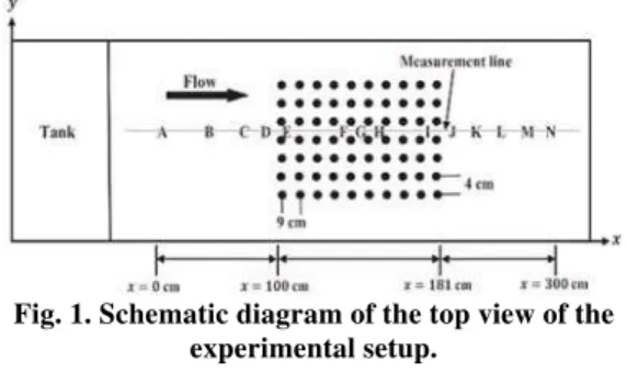
Fig. 1. Schematic diagram of the top view of the experimental setup.

2. E

M

2.1 Details of Experimental Design

a calibrated V-Notch. A honeycomb baffle wall was provided at the entrance of the flume to reduce the turbulence and non-uniformity in the incoming flow. Depth measurements were made by using a point gauge with the attachment of graduated millimeter scale. The point gauge with accuracy ±0.01 cm was first set to the bed level with zero scale and the depth was measured by moving the pointer to the free surface. The bed surface of the flume was made rough by cladding sand particles of size

50 0.25 cm.

D 

2.2 Model of Vegetation Patch

The test section was considered as 300 cm long which starts at 700 cm from the entrance of the flume. The vegetation patch was located at the middle region of test section as well as the central area of the cross-sectional area of the flume. The vegetation characteristics of the patch were emergent, rigid and sparse. It was made by seventy uniform acrylic cylindrical rods with dimensions 0.64 cm diameter and 30 cm length. The rods were planted perpendicularly as an array of 7 × 10 on a perspex sheet which was fixed to the channel bed. In the patch, uniform spacings of 9 cm and 4 cm were maintained between centers of two consecutive cylinders along streamwise and lateral directions respectively. The dimensions of the patch were 81 cm long and 24 cm wide. Figs. 1 and 2 clarify the setup of the vegetation patch in the flume.

2.3 Data Collection

A three-dimensional (3-D) Acoustic Doppler Velocimeter (ADV) with four down looking probes was used to measure the point velocities across the channel section. Table 1 shows a brief summary of the experimental conditions. The Nortek Vectrino plus measured the instantaneous velocities of water by the reflected sound from the natural suspended dirt particles in the water. Fig. 2 presents a photograph of one of the experiments performed. Since the center of the measuring volume of the ADV predicts the flow velocity, therefore the spatial resolution of the Nortek Vectrino plus permitted measurement 0.3 cm above from the channel bed. The size of the sampling volume of the measurement was 2.5 cubic cm. The down-looking ADV measured the flow velocities in the remote sampled volume at a distance of 0.05 m away to minimize the probe disturbance in the flow. To allow the stabilization of the flow field, the velocity measurement was taken 30 minutes after the flow was commenced. To analyze the uncertainty of the measurements, samples were taken at a location 7.7 cm above the channel bed at different times after starting the experiments. The computed uncertainty estimates of root-mean-square velocities and Reynolds shear stresses were 3% and 15% respectively. Along the centreline of the open channel through its cross sectional area, the three-dimensional velocities were measured in 100 cm upstream, interior and 100 cm downstream of the vegetation patch. Table 2 shows the stations along streamwise direction at which vertical distribution of three-dimensional velocities were measured. The water depth h was kept 15 cm and at each station, velocity was measured for 15

points along vertical direction which were 0.3, 0.5, 0.7, 0.9, 1.5, 2, 2.5, 3, 4, 5, 6, 7, 8, 9 and 10 cm above from the channel bed. The sampling rate was 100 Hz and the data was collected for 120 seconds duration at each vertical location and this implies that 100 × 60 × 2 = 12000 instantaneous velocity data points were captured at each measuring point. When the ADV was moved from one vertical location to the next measuring point, the flow field may be disturbed in the vicinity due to the movement of ADV. Therefore, two minutes of time interval were taken in between velocity measurements of two consecutive vertical locations so that the disturbance of the flow field can be neutralized.

Table 1 Turbulent flow conditions of experiment

Flow depth (h) 15 cm Average flow velocity 29 cm/s Maximum flow velocity 30 cm/s Shear velocity 0.30 cm/s Froude Number 0.234 Reynolds number (Re) 43500

Vegetation length (x) 81 cm Vegetation length (y) 24 cm Diameter of cylinders 0.64 cm

Number of cylinders 70 Space between two cylinders (x) 9 cm Spacing between two cylinders (y) 4 cm

Vegetation density 0.0178/cm

2.4 Post Processing of Data

For the post processing of data obtained from the ADV, a three-dimensional coordinate system has been adopted where x, y and z denoted streamwise, transverse and vertical directions respectively. The coordinate system can be well understood from Fig. 2. Spike filtering, correlation and signal-to-noise ratio (SNR) thresholding techniques were used as suggested by Chanson et al. (2008) to minimize the effect of the Doppler noise in the data. To further improve the accuracy of the turbulence measurements, low correlations and low SNR data were removed. The basic ideas of Goring and Nikora (2002), Wahl (2003) and Mori et al. (2007) for removing the random spikes were implemented. The spikes in velocity measurements removed from the raw time series were replaced by applying cubic polynomial interpolation. The number of interpolated points consisted less than 5% of the original velocity record and had no effect on the spectrum and overall frequency content.

Fig. 2. Set-up of the laboratory experiment.

3. E

R

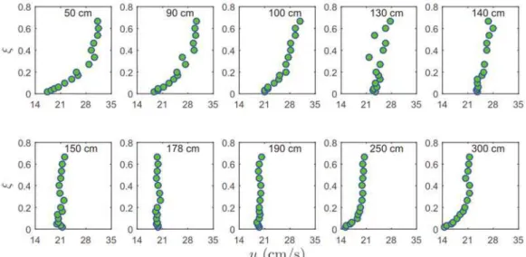
Fig. 3. Nature of time averaged streamwise velocity u at upstream (x = 50 and 90 cm), interior (x = 100, 130, 140, 150 and 178 cm) and downstream (x = 190, 250 and 300 cm) of the vegetation patch.

Table 2 Locations of instantaneous flow velocity measurements along streamwise direction

A B C D E F G H I J K L M N

x (cm) = 0 50 80 90 100 130 140 150 178 190 22 0

25 0

28 5

30 0 Upstream of vegetation Interior of vegetation Downstream of vegetation

along x, y and z directions are denoted as u, v and w. The fluctuation parts of u, v and w are represented by u′, v′ and w′ respectively. In this section, the underlying physics governing the turbulent characteristics of measured data in sparsely vegetated open channel flow is explained comprehensively. The organization of this section is given here. First, the underlying physics of the nature of flow velocity has been uncovered. Second, the behavior of three normal stresses has been interpreted. Third, the characteristics of Reynolds shear stress are discussed. Next, the variation of turbulent kinetic energy profiles is discussed. Finally, a comparison analysis between the profiles of time-space averaged turbulent features inside the vegetation patch and the corresponding profiles of fully developed flow without the patch has been performed.

3.1 Time Averaged Streamwise Velocity

Figure 3 reveals the profiles of time averaged streamwise velocity u with normalized vertical height (= z/h) from the channel bed. It is observed that u shows positive values throughout the flow depth at all locations in upstream, interior and downstream regions of the vegetation patch. At up-stream of the patch, the profiles of u at x = 50 and 90 cm indicate the existence of fully developed flow without vegetation. At the leading edge of the patch (x = 100 cm), the profile of u exhibits a little deviation in the flow region where > 0.2 from its fully developed nature without vegetation. The cylinders located at the leading edge of the vegetation patch might have a crucial role to affect the u profile there. After entering into the vegetation

Fig. 4. Nature of time averaged lateral velocity v at upstream (x = 50 and 90 cm), interior (x = 100, 130, 140, 150 and 178 cm) and downstream (x _{= 190, 250 and 300 cm) of the vegetation patch.}

Fig. 5. Nature of time averaged vertical velocity w at upstream (x = 50 and 90 cm), interior (x = 100, 130, 140, 150 and 178 cm) and downstream (x = 190, 250 and 300 cm) of the vegetation patch.

patch. The resistance force owing to the stems inside the patch is responsible for the decreased magnitude of the u profiles. Unlike the decreasing trend of u magnitude inside the patch and after crossing it, it is noticed that the magnitude of u increases at the far downstream of the trailing edge (x = 250 and 300 cm) as the flow endeavors to recover its fully developed nature which is found in upstream of the vegetation patch.

3.2 Time Averaged Lateral Velocity

Figure 4 illustrates the vertical distribution of measured time averaged profiles of transverse velocity v. It is observed that v shows positive values everywhere except x = 50 cm which is situated at upstream of the vegetation patch. From the leading edge of the vegetation patch represented by x = 100 cm, it is followed that the magnitude of v increases with increasing streamwise length up to the first half length of vegetation patch i.e. x = 140 cm. The

number of vortices increases owing to the interaction between flow and the cylinders of vegetation patch. Those vortices increase the intensity of the secondary current inside the patch, hence the magnitude of v increases. Apart from this, it is noticed that after crossing the half length of vegetation patch, a propensity of decreasing magnitude of v is observed for the rest part of downstream vegetation patch and also far from its trailing edge i.e. x = 150 to 300 cm. The probable reason behind this characteristic is that the intensity of secondary current decreases along the centerline of vegetation patch as the flow deviates from the central region towards the sidewalls owing to the resistance offered by the cylinders.

3.3 Time Averaged Vertical Velocity

zero at upstream of the vegetation located by x = 50 cm and this characteristic proves the existence of uniform open channel flow at the upstream of vegetation patch. As the flow approaches the vegetation patch, w shows a decreasing nature and reaches the lowest profile at the leading edge of the patch denoted by x = 100 cm. This phenomenon indicates the presence of downward flow at the upstream of the patch similar to flow over highly rough bed surfaces. Moreover, the three-dimensional characteristic of flow field near the leading edge of the vegetation patch i.e. x = 90 cm can be perceived by the equal magnitude and opposite signs of v and w profiles. At leading edge of the vegetation patch, w is minimum in terms of its value and after flow entering into the vegetation patch, w increases inside the vegetation patch and interestingly this characteristic is continued up to x = 190 cm which is the immediate wake region after crossing the trailing edge of the patch. It has been perceived that the down-ward vertical flow losses its strength as it is considerably affected by the cylinders inside the sparse vegetation patch. The increased values of w in the wake region explains that the streamlines follow the downward flow and their behavior is similar to the turbulent flow over rough beds.

Fig. 6. Nature of streamwise normal stress u2at upstream (x = 50 and 90 cm), interior (x = 100, 130, 140, 150 and 178 cm) and downstream (x = 190, 250 and 300 cm) of the vegetation patch.

Fig. 7. Nature of lateral normal stress v2at upstream (x = 50 and 90 cm), interior (x = 100, 130, 140, 150 and 178 cm) and downstream (x = 190, 250 and 300 cm) of the vegetation patch.

3.4 Normal Stresses

Figures 6, 7 and 8 show the profiles of streamwise normal stress u2 , lateral normal stress v2 and vertical normal stress w2 at different streamwise locations of the upstream, interior and downstream of the vegetation patch. At the leading edge of the vegetation patch i.e. x = 100 cm, it is observed that the

three normal stresses illustrate the same behavior similar to a fully developed flow over a rough bed where the maximum value occurs in the velocity defect layer near the channel bed together with decreasing magnitude with increasing vertical distance from the bed. The magnitudes of normal stresses inside the vegetation patch (x = 130, 140, 150 and 178 cm) show higher value in comparison to the corresponding magnitudes of normal stresses which are found in the region upstream of the vegetation patch. The intense turbulent mixing and increased vorticity inside the vegetation patch are responsible for the higher fluctuations of stream-wise, lateral and vertical velocities of flow, therefore large values of u 2,v2, and w2 are obtained in the interior of the patch. Unlike the fully developed flow without vegetation where the maximum value of normal stress occurs near the channel bed, the peak values of u 2,v2,and w2 are found to be occurring far from the channel bed inside the vegetation patch. The reason behind this phenomenon is that a large number of swirling vortices move from the channel bed to the free surface of the flow and the swirling motion causes higher fluctuations in the flow region which is located far away from the channel bed. Interestingly, after crossing one immediate length from the trailing edge of the vegetation patch i.e. x = 190 cm, the magnitudes of u 2,v2,and w2 are found to be decreased with respect to the corresponding profiles inside the vegetation patch which implies lesser turbulent fluctuations of flow velocity after crossing the vegetation patch. In addition, it is noticed that the magnitudes of u 2,v2, and w2 observed far downstream from the vegetation patch are small with respect to the corresponding values which are found at upstream and interior of the patch. This characteristic of normal stresses apprises that with increasing downstream length from the patch, the flow tries to recover its fully developed uniform nature without vegetation. Overall, inside the vegetation patch, the values of u2 and v2 lie in the range of 5 to 30

2 2

cm /s whereas the magnitude of w2 are in the range of 1 to 6 cm /2 s2The decreased magnitude of vertical normal stress in reference to the values of streamwise and lateral normal stresses asserts the anisotropy of turbulence inside the vegetation patch.

190, 250 and 300 cm) of the vegetation patch.

Fig. 9. Nature of Reynolds shear stress -u w at upstream (  x = 50 and 90 cm), interior (x = 100, 130, 140, 150 and 178 cm) and downstream (x = 190, 250 and 300 cm) of the vegetation patch.

Fig. 10. Nature of turbulent kinetic energy k at upstream (x = 50 and 90 cm), interior (x = 100, 130, 140, 150 and 178 cm) and downstream (x = 190, 250 and 300 cm) of the vegetation patch.

3.5 Reynolds Shear Stress

Vertical distribution of Reynolds shear stress u w  along the streamwise direction is shown in Fig. 9. The profiles of other two Reynolds shear stresses

u v 

 and v w are not shown since they do not play a significant role in the flow field in comparison to

u w 

 . It is observed that up to the entrance of vegetation patch represented by x = 100 cm, the profiles of u w  display same magnitude and those profiles attain peak values within the wall shear layer due to prevalence of sweeps and ejections. Therefore, inside the vegetation patch (x = 130, 140, 150 and 178 cm), with increasing downstream distance from the leading edge, the magnitude of

u w 

 profile decreases in comparison to the preceding profile. The decreasing characteristic may

be governed by the occurrence of inward and out-ward events in addition to sweeps and ejections. It is worth mentioning here that after leaving the trailing edge of the vegetation patch also, the magnitude of Reynolds shear stress profiles (x = 190, 250 and 300 cm) decrease with increasing downstream length; however the order of decreasing magnitude at downstream of the patch is small in comparison to the order inside that patch.

3.6 Turbulent Kinetic Energy

near the channel bed as the turbulence is very high due to the effect of the bed roughness. As the flow

Fig. 11. Comparison between time-space averaged (TSA) turbulent quantities within the vegetation patch and corresponding fully developed (FD) profiles without vegetation.

enters into the vegetation patch, though the profiles of k start to show some inconsistent nature, but the magnitude of those k profiles increases with increasing downstream length up to x = 150 cm. Moreover, in this region, it is observed that the profiles of k exhibit the corresponding maximum values far from the channel bed. This could be due to the movement of the center of vortices near the free surface resulting from the upward ejection of swirling eddies which are generated at the bed surface. Therefore, in comparison to the velocity fluctuations near the channel bed, higher fluctuations occur in the flow region which is located far from the channel bed and results large magnitude of k. On the other hand, it is followed that after crossing the region denoted by x = 150 cm, the magnitude of k decreases with increasing downstream length; however unlike the inconsistent behavior in the first half of the vegetation patch, the profiles of k gradually develop a consistent characteristic in the long segment of flow represented by x = 178 to 300 cm. It is noticed that though the order of decreasing magnitude of k is small inside the vegetation patch and the wake region downstream of trailing edge, but the magnitude decreases rapidly far downstream from the patch (x = 250 and 300 cm) since in this region, the flow endeavors to recover its fully developed nature without vegetation.

3.7 Time-Space Averaged Turbulence

Quantities

In this section, the time-space averaged (TSA) approach has been used to understand the overall difference between the turbulent flow inside the sparse vegetation patch and the fully developed flow (FDF) without vegetation. The TSA profile of each turbulent feature is obtained by the spatial averaging of corresponding time averaged profiles measured

inside the vegetation patch (x = 100, 130, 140, 150 and 178 cm). Fig. 11 compares the TSA profiles of several turbulent features with the corresponding vertical distributions of FDF without vegetation at x = 0 cm.

Figures 11(a), 11(b) and 11(c) illustrate that the magnitudes of TSA of streamwise, lateral and vertical velocities decrease with respect to the corresponding FDF profiles without vegetation which supports the hypothesis that the sparse vegetation patch influences the velocity distribution and causes the higher turbulence damping near the bed and resistance to the flow in the outer region, in feedback increased magnitudes of normal stresses

2_, 2_,

u v and w2at interior of the patch which is reflected in Figs. 11(d) to 11(f). In FDF, unlike the decreasing magnitude of normal stresses with increasing vertical height from the channel bed, normal stresses of TSA increases with increasing vertical distance from the bed. This characteristic confirms the increased turbulence mixing and dissipation of momentum far from the bed in the interior of the patch.

The comparison of the Reynolds shear stress u w  for TSA and FDF is shown in Fig. 11(g). For TSA profile inside the vegetaion, smaller magnitude of

u w 

 is observed in comparison to FDF without the vegetation. This phenomenon indicates that over an erodible sediment bed, the bed friction will be reduced inside the vegetation patch which results decreased bed load transport rate and increased sediment deposition in the patch.

Figure 11(h) displays that except near the channel bed, the magnitude of TSA turbulent kinetic energy k profile in the sparse vegetation patch is more than the value of k for FDF without vegetation. Besides this, the TSA profile of k increases towards free surface which is contrary to the fully developed flow without vegetation where k decreases with increasing vertical distance from the channel bed. The characteristic confirms the occurrence of turbulent bursting events throughout the flow depth in the sparse vegetation patch.

4. M

M

It is a well known fact that the log-law is not applicable to the rectangular velocity profile of fully mixed turbulent flow at interior of the emergent vegetation patch. Barenblatt (1993) proposed a velocity profile applicable to the overlap layer of pipe flow in terms of viscous length scales together with an assumption that the flow in the overlap layer is a function of Reynolds number. By considering the velocity profile of Barenblatt (1993) as a reference, a modified mathematical equation in terms of outer layer scaling is proposed here to estimate the velocity distribution inside the sparse vegetation patch.

3

ln(Re)

1 2

[ ln(Re) ]

C

m

u

C C

u   (1)

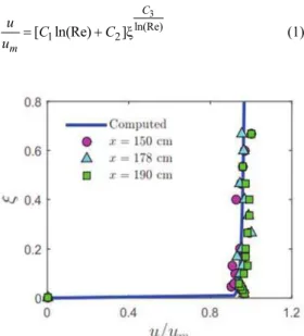
Fig. 12. Comparison of Eq. (1) with experimental data observed at x = 150, 178 and 190 cm.

In Eq. (1), u is scaled with the maximum velocity um obtained from the measured values at the station and

1

C , C₂and C₃ are empirical parameters which need to be evaluated from the experimental data. Velocity profile along the depth at x = 150 cm is fitted

with Eq. (1) by ‘lsqcurvefit’ function in MAT-LAB and the values of C₁, C₂and are computed as

−0.922, 10.81 and 0.127 respectively together with the coefficient of determinationR20.99. Fig. 12 shows the comparison of computed values with experimental data and a good agreement is observed between them. Apart from this, Eq. (1) is also verified with the measured velocity profiles at x = 178 and 190 cm and the computed values approximate those measured data with R20.99. It appears from Eq. (1) that in fully mixed vegetation flow, viscous effects are negligible and the flow region is similar to the typical free surface layer where the turbulent kinetic energy dissipation exceeds the turbulent kinetic energy production rate. In this region, velocity is almost same for most of the depth and velocity defect is negligible. From velocity profiles, it appears that the wall shear layer is negligibly thin in the fully mixed vegetated flow.

5. CONCLUSIONS

In this paper, an experimental investigation has been preformed to predict the turbulent features through an emergent and sparsely vegetated open channel turbulent flow. The conclusions obtained are given as follows.

 The magnitude of streamwise velocity increases with increasing steamwise length inside the vegetation; however a fully developed rectangular velocity profile is observed when the flow crosses the first half length of the patch from upstream and it is continued up to a certain length after the trailing edge of the patch.

 Inside the vegetation patch, the magnitude of lateral velocity increases with increasing streamwise length up to the first half length of the patch and further downstream, its magnitude decreases with increasing length.

 It has been noticed from the time-space averaging approach that inside the vegetation patch, the magnitudes of streamwise, lateral and vertical velocities decrease in comparison to the profiles of fully developed flow without vegetation; however the decreased values of velocities in the interior of vegetation are compensated by the increased magnitudes of streamwise, lateral and vertical normal stresses respectively in that flow region.

 The normal stresses are increasing inside the vegetation patch in comparison to the fully developed flow without vegetation. Moreover, the magnitude of streamwise and lateral normal stresses are five times greater than that of vertical normal stress.

 With increasing downstream distance in the first half length of vegetation patch, the magnitude of turbulent kinetic energy profile increases with peak value located far from the bed. In the second half length, the profiles of turbulent kinetic energy show nonuniform decreasing characteristic with increasing down-stream distance.

 A mathematical model is developed for the fully mixed streamwise velocity profile inside the sparse vegetation patch and the proposed model approximates the experimental data accurately.

 Finally, it can be concluded that this study has a significant contribution to understand the physics of turbulent features inside a sparsely vegetated open channel turbulent flow.

A

Debasish Pal received financial assistance from SRIC Project of IIT Kharagpur (Project code: FVP).

R

Banerjee, T., M. Muste and G. Katul (2015). Flume experiments on wind induced flow in static water bodies in the presence of protruding vegetation. Advances in Water Resources 76, 11–28.

Barenblatt, G. (1993). Scaling laws for fully developed turbulent shear flows. part 1. basic hypotheses and analysis. Journal of Fluid Mechanics 248, 513–520.

Bernardini, M., S. Pirozzoli and P. Orlandi (2014). Velocity statistics in turbulent channel flow up to Reτ = 4000. Journal of FluidMechanics 742, 171–191.

Chanson, H., M. Trevethan and S. I. Aoki (2008). Acoustic doppler velocimetry (adv) in small estuary: field experience and signal post-processing. Flow Measurement and Instrumentation 19(5), 307–313.

Cheng, N. S. (2013). Calculation of drag coefficient for arrays of emergent circular cylinders with pseudofluid model. Journal of Hydraulic Engineering 139(6), 602–611.

Cheng, N. S., H. Nguyen, S. K. Tan and S. Shao (2012). Scaling of velocity profiles for depth-limited open channel flows over simulated rigid vegetation. Journal of Hydraulic Engineering 138(8), 673–683.

Coles, D. (1956). The law of the wake in the turbulent boundary layer. Journal of Fluid Mechanics 1(2), 191–226.

Fischer, H. B. (1973). Longitudinal dispersion and turbulent mixing in open-channel flow. Annual Review of Fluid Mechanics 5(1), 59–78. Ghisalberti, M. and H. Nepf (2009). Shallow flows

over a permeable medium: the hydrodynamics of submerged aquatic canopies. Transport in

Porous Media 78(2), 309–326.

Goring, D. G. and V. I. Nikora (2002). Despiking acoustic doppler velocimeter data. Journal of Hydraulic Engineering 128(1), 117–126. Guo, J. and P. Y. Julien (2008). Application of the

modified log-wake law in open-channels. Journal of Applied Fluid Mechanics 1(2), 17– 23.

Guo, Y. (2016). Flow in open channel with complex solid boundary. Journal of Hydraulic Engineering 142(2).

Kundu, S. and K. Ghoshal (2013). An explicit model for concentration distribution using biquadratic-log-wake law in an open channel flow. Journal of Applied Fluid Mechanics 6(3), 339–350. Lopez, F. and M. H. Garcia (2001). Mean flow and

turbulence structure of open-channel flow through non-emergent vegetation. Journal of Hydraulic Engineering 127(5), 392–402. Mori, N., T. Suzuki and S. Kakuno (2007). Noise of

acoustic doppler velocimeter data in bubbly flows. Journal of Engineering Mechanics 133(1), 122–125.

Musleh, F. A. and J. F. Cruise (2006). Functional relationships of resistance in wide flood plains with rigid unsubmerged vegetation. Journal of Hydraulic Engineering 132(2), 163–171. Nepf, H. M. (2012a). Flow and transport in regions

with aquatic vegetation. Annual Review of Fluid Mechanics 44, 123–142.

Nepf, H. M. (2012b). Hydrodynamics of vegetated channels. Journal of Hydraulic Research 50(3), 262–279.

Nezu, I. and W. Rodi (1986). Open-channel flow measurements with a laser doppler anemometer. Journal of Hydraulic Engineering 112(5), 335– 355.

Osterkamp, W. R., C. R. Hupp and M. Stoffel (2012). The interactions between vegetation and erosion: new directions for research at the interface of ecology and geomorphology. Earth Surface Processes and Landforms 37(1), 23–36. Pu, J. H. (2013). Universal velocity distribution for smooth and rough open channel flows. Journal of Applied Fluid Mechanics 6(3), 413–423. Rominger, J. T. and H. M. Nepf (2011). Flow

adjustment and interior flow associated with a rectangular porous obstruction. Journal of Fluid Mechanics 680, 636–659.

Stone, B. M. and H. T. Shen (2002). Hydraulic resistance of flow in channels with cylindrical roughness. Journal of Hydraulic Engineering 128(5), 500–506.

Wahl, T. L. (2003). Discussion of despiking acoustic doppler velocimeter data by derek g. goring and vladimir i. nikora. Journal of Hydraulic Engineering 129(6), 484-487.

White, B. L. and H. M. Nepf (2008). A vortex- based model of velocity and shear stress in a partially vegetated shallow channel. Water Resources Research 44(1).

White, B. L. and H. M. Nepf (2008). Shear in-stability and coherent structures in shallow flow adjacent to a porous layer. Journal of Fluid

Mechanics 593, 1–32.

Yang, J. Q., F. Kerger and H. M. Nepf (2015). Estimation of the bed shear stress in vegetated and bare channels with smooth beds. Water Resources Research 51(5), 3647–3663. Yang, S. Q., S. K. Tan and S. Y. Lim (2004).