On the applicability of conventional transmission line theory within cavities

www.adv-radio-sci.net/4/117/2006/ © Author(s) 2006. This work is licensed under a Creative Commons License.

Radio Science

On the applicability of conventional transmission line theory

within cavities

F. Gronwald

Institute for Fundamental Electrical Engineering and EMC, Otto-von-Guericke-University Magdeburg, Universit¨atsplatz 2, 39106 Magdeburg, Germany

Abstract.We investigate whether or not conventional trans-mission line theory needs to be modified if transtrans-mission lines are considered that are located in a cavity rather than in free space. Our analysis is based on coupled Pocklington’s equa-tions that can be reduced to integral equaequa-tions for the an-tenna mode and the transmission line mode. Under the usual assumptions of conventional transmission line theory these modes do approximately decouple within a cavity. As a re-sult, cavity properties will primarily influence the antenna mode but not the transmission line mode.

1 Introduction

Interior problems of Electromagnetic Compatibility analysis involve electric and electronic components that are located within cavities (Tesche et al., 1997; Lee, 1995). Usually, transmission lines will constitute a part of these components. To model the electromagnetic propagation along transmis-sion lines we have to resort to the Maxwell theory. It is de-sirable to simplify Maxwell’s equations to Telegrapher equa-tions since soluequa-tions of Telegrapher equaequa-tions are fairly easy to obtain. But in case of interior problems we have to ex-amine if these simplification can be made inside a cavity and this is the subject of this paper. Our strategy will be to exhibit the steps that are necessary to derive conventional transmis-sion line theory from integral equations of antenna theory. There already is a number of such derivations (see, for exam-ple, King, 1955; Tkachenko et al., 1995; Tesche et al., 1997; Haase et al., 2004). These approaches use electric field inte-gral equations as physical basis but differ in the assumptions and approximations that are made in order to arrive at the conventional transmission line theory. Also they assume, im-plicitly or exim-plicitly, that the transmission lines are located in

Correspondence to:F. Gronwald ([email protected])

free space. The distinctive feature of our approach is that we take advantage of a separation of antenna mode currents and transmission line mode currents right from the beginning.

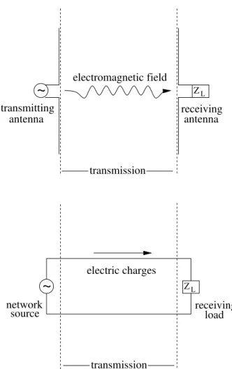
Conventional transmission lines are metallic structures that transmit electromagnetic signals and energy. In this spect they are very similar to systems of transmitting and re-ceiving antennas. However, the physical mechanisms that govern the electromagnetic transmission along transmission lines is quite different if compared to the electromagnetic transmission between pairs of antennas, compare Fig. 1.

In between a pair of antennas the electromagnetic trans-mission results from a propagating electromagnetic field which, for practical purposes, can often be approximated by a radiation field. This does not mean that in such a situation no Coulomb fields are present. Coulomb fields will be related to the electric charges that move along the antennas and con-stitute their near-fields. But in many cases the transmitting and receiving antennas are sufficiently far apart such that the main coupling is mediated by the radiation field which re-sembles a freely propagating electromagnetic field. Electric charges are not involved in the actual electromagnetic trans-mission that happens in between the antennas. They only are required at the beginning and at the end of the transmission in order to, respectively, generate and receive the transmit-ting electromagnetic field.

~

transmitting antenna

~

network

source receivingload

transmission electric charges

receiving antenna electromagnetic field

transmission

Fig. 1.Electromagnetic transmission by means of a pair of antennas (upper part) and a transmission line (lower part). In between the antennas an electromagnetic field mediates the actual transmission while the transmission line provides electric charges that mediate the transmission between the source and the load.

and negligible. Therefore, in the conventional transmission line theory focus is put on the electric charges and their ac-companying Coulomb fields.

The conventional transmission line theory can be derived from the Maxwell theory as a limiting case and contains the electric current, representing electric charges, and the elec-tric voltage, representing the associated Coulomb fields, as main physical quantities. Clearly, these two quantities are not independent of each other. They are related by the Tele-grapher equations, which constitute a set of coupled first or-der differential equations, and are much easier to solve than the Maxwell equations.

In the derivation of the Telegrapher equations from the Maxwell equations it is customary to consider some, a pri-ori, arbitrary transmission line and to assume a number of restrictions (Tesche et al., 1997):

1. The conductors are geometrically uniform, i.e. the transmission line is not curved or bent.

2. The distance between the conductors of the transmis-sion line is small compared to the wavelength of the ex-citing electromagnetic field.

3. The thickness of the conductors of the transmission is small if compared to the wavelength of the exciting electromagnetic field.

4. The conductors are perfectly conducting.

The second and third of these restrictions are not clearly cut since “smallness” with respect to a wavelength is not a pre-cise notion. The reason for these approximate criteria is that, in fact, one would like to remove the influence of radiation fields on the transmission line. However, Coulomb fields and radiation fields are inseparably intertwined. Therefore, in the conventional transmission line theory, one only takes into ac-count electromagnetic interactions between electric charges at short distances where Coulomb fields dominate and radi-ation fields can be neglected. Also the first and fourth re-striction are put forth to avoid an influence of radiation fields on the transmission line. In contrast to the second and third restriction they can be formulated in a mathematically exact way with no approximations involved. Since in the derivation of the Telegrapher equations approximations are inevitable it is often acceptable to relax the first and fourth conditions to some degree and allow for transmission lines which are slightly bent, i.e. which are characterized by radii of curva-ture that are large compared to the wavelength of the exciting field, and which are good conducting rather than perfectly conducting, i.e. which are characterized by a conductivityσ that fulfills the requirement|σ| ≫ |εω|.

It has been mentioned that in the derivation of the conven-tional transmission line theory it usually is assumed that the transmission line is located in free space. It follows that in the derivation of the Telegrapher equations the Green’s func-tion of free space is employed. If we want to consider a transmission line within a resonating environment we may employ a cavity’s Green’s function rather than the Green’s function of free space. Thus, it is necessary to check if this modification has an influence on the validity of the Telegra-pher equations of the conventional transmission line theory.

2 Coupled Pocklington’s equations, antenna and transmission line mode

We consider a set of coupled Pocklington’s equations that models the electromagnetic coupling to a system of wires and represents a transmission line. For concreteness we consider two wires and assume a thin-wire approximation. Then the corresponding coupled Pocklington’s equations are given by Nakano (1996)

j ωµ

Z

wire 1

GE(τ1, τ1′)I1(τ1′) dτ1′

+

Z

wire 2

GE(τ1, τ2′)I2(τ2′) dτ2′

·e_τ

1 =E

inc

tan(τ1) , (1)

j ωµ

Z

wire 1

GE(τ2, τ1′)I1(τ1′) dτ

′

1

+

Z

wire 2

GE(τ2, τ2′)I2(τ2′) dτ

′

2

·e_τ

2 =E

inc

tan(τ2) . (2)

Here we introduced the variablesτ1,τ2that parameterize the

length of wire 1 and wire 2, respectively. Fixed values of these variables represent fixed wire positions. The unit vec-torse_τ

1,eτ1 are tangent to the line-like wires atτ1,τ2. The currentsI₁(τ1),I2(τ2)result from the thin-wire

approxima-tion and are defined by

I_i(τi):=Iieτi (3)

fori=1,2. The scalarIi is the value of the electric current at the wire positionτi. Finally, we denote byG

E

the dyadic Green’s function for the electric field (Tai, 1994).

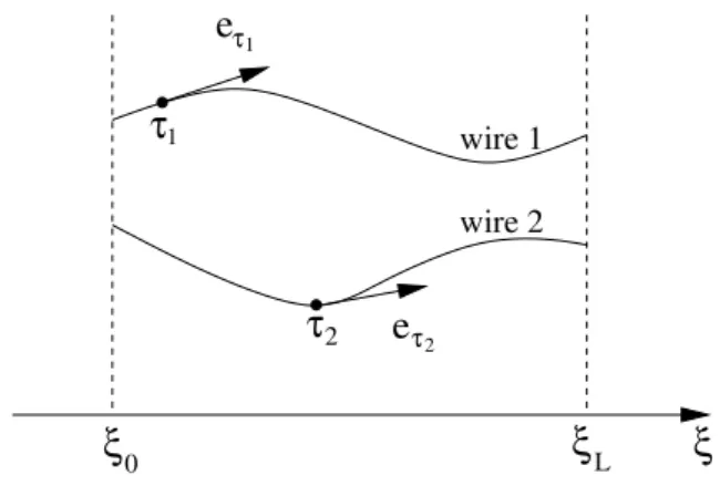
If the wires form a transmission line we expect that they can be parameterized by a common coordinateξwithξ=ξ0

at the beginning andξ=ξLat the end of the line, compare Fig. 2. We take this coordinate as a common integration vari-able and write Eqs. (1) and (2) as

j ωµ

Z ξL

ξ0

GE(τ1, τ1′)I1(τ1′)

∂τ₁′ ∂ξ′

+GE(τ1, τ2′)I2(τ2′)

∂τ₁′ ∂ξ′

dξ′

·e_τ

1 =E

inc

tan(τ1) , (4)

j ωµ

Z ξL

ξ0

GE(τ2, τ1′)I1(τ1′)

∂τ₁′ ∂ξ′

+GE(τ2, τ₂′)I2(τ₂′)

∂τ₂′ ∂ξ′

dξ′

·e_τ

2 =E

inc

tan(τ2) . (5)

The variablesτ1,τ2are now understood as functions of the

parameterξ.

Next we introduce two currentsI_AandI_{TLas linear}

com-binations ofI_1andI_2,

I_A:= 1₂(I₁+I₂) , (6)

I_TL := 1₂(I₁−I₂) . (7)

ξ

ξ

ξ

τ

e

wire 2 wire 1

τ1

e

1

Fig. 2. Introduction of a common variableξ which parameterizes the wires of a transmission line.

The inverse equations are

I₁=I_A+I_TL, (8)

I₂ =I_A−I_TL. (9)

These identifications are well-known from the conventional transmission line theory whereI_{A represents the so-called}

“antenna mode” or “common mode” andI_TLrepresents the so-called “tranmission line mode” or “differential mode”. In our present context these identifications are still formal. We note that neitherI_AnorI_{TLneed to be tangent to one of the}

wires. But it is clear that we still may splitI_AandI_{TLinto a}

component and a unit vector,

I_A= 1

2 I1eτ1+I2eτ2

=:IAeIA, (10)

I_TL= 1

2 I1eτ1−I2eτ2

=:ITLeIT L. (11)

If the relations (8) and (9) are inserted into Eqs. (4) and (5) it is simple to find

j ωµ

Z ξL

ξ0

GE(τ1, τ1′)

∂τ₁′ ∂ξ′ +G

E (τ1, τ2′)

∂τ₂′ ∂ξ′

I_A(ξ′)

+

GE(τ1, τ1′)

∂τ₁′ ∂ξ′ −G

E (τ1, τ2′)

∂τ₂′ ∂ξ′

I_TL(ξ′)

dξ′

·e_τ

1

=E_taninc(τ1) , (12)

j ωµ

Z ξL

ξ0

GE(τ2, τ1′)

∂τ₁′ ∂ξ′ +G

E (τ2, τ2′)

∂τ₂′ ∂ξ′

I_A(ξ′)

+

GE(τ2, τ1′)

∂τ₁′ ∂ξ′ −G

E (τ2, τ2′)

∂τ₂′ ∂ξ′

I_TL(ξ′)

dξ′

·e_τ

2

We both add and subtract these equations and obtain

j ωµ

Z ξL

ξ0

GE_+A(τ1, τ2, τ1′, τ

′

2)IA(ξ′)

+GE_+TL(τ1, τ2, τ1′, τ2′)ITL(ξ′)

dξ′

=Einc_tan(τ1)+Etaninc(τ2) , (14)

j ωµ

Z ξL

ξ0

GE_−A(τ1, τ2, τ1′, τ

′

2)IA(ξ′)

+GE_−TL(τ1, τ2, τ1′, τ

′

2)ITL(ξ′)

dξ′

=Einc_tan(τ1)−Etaninc(τ2) , (15)

where we introduced the abbreviations

GE_+A(τ1, τ2, τ1′, τ2′):= (16) e_τ

1·

GE(τ1, τ1′)

∂τ₁′ ∂ξ′ +G

E (τ1, τ2′)

∂τ₂′ ∂ξ′

·e_I A

+e_τ

2·

GE(τ2, τ1′)

∂τ₁′ ∂ξ′ +G

E (τ2, τ2′)

∂τ₂′ ∂ξ′

·e_I A,

GE_+TL(τ1, τ2, τ1′, τ2′):= (17) e_τ

1·

GE(τ1, τ₁′)

∂τ₁′ ∂ξ′ −G

E (τ1, τ₂′)

∂τ₂′ ∂ξ′

·e_I TL

+e_τ

2 ·

GE(τ2, τ1′)

∂τ₁′ ∂ξ′ −G

E (τ2, τ2′)

∂τ₂′ ∂ξ′

·e_I TL,

GE_−A(τ1, τ2, τ1′, τ

′

2):= (18)

e_τ

1·

GE(τ1, τ1′)

∂τ₁′ ∂ξ′ +G

E (τ1, τ2′)

∂τ₂′ ∂ξ′

·e_I A

−e_τ

2·

GE(τ2, τ₁′)

∂τ₁′ ∂ξ′ +G

E (τ2, τ₂′)

∂τ₂′ ∂ξ′

·e_I A,

GE_−TL(τ1, τ2, τ1′, τ

′

2):= (19)

e_τ

1·

GE(τ1, τ1′)

∂τ₁′ ∂ξ′ −G

E (τ1, τ2′)

∂τ₂′ ∂ξ′

·e_I TL

−e_τ

2 ·

GE(τ2, τ1′)

∂τ₁′ ∂ξ′ −G

E (τ2, τ2′)

∂τ₂′ ∂ξ′

·e_I TL.

3 Decoupling of antenna and transmission line mode in free space

The expressions we obtained so far look more complicated than the original Eqs. (1) and (2) that we started from. To nevertheless appreciate this form of the coupled Pockling-ton’s equations we specialize to the case of straight and par-allel wires. Then we may align a Cartesian coordinate system

z1

z ’2

z ’1

z2

z

z’

z

|z − z’ |1

|z − z’ |2

|z − z’ |2

|z − z’ |₁

1

z

z

wire 1 wire 2 2 2 1

y

d

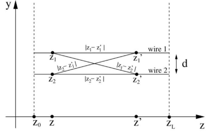
Fig. 3.Geometry of a straight two-wire transmission line.

such that thez-axis is parallel to the wires and may choose ξ =z. This leads to the simplifications

e_τ

1 =eτ2 =eIA=eIT L, (20)

e_τ

1,2 ·G E

·e_I

A,TL =G E

zz, (21) ∂τ1

∂ξ = ∂τ2

∂ξ =1. (22)

Accordingly, Eqs. (16) – (19) reduce to GE_+A(z1, z2, z′1, z

′

2)=G

E

zz(z1, z′1)+G

E zz(z1, z′2)

+GE_zz(z2, z′1)+G

E

zz(z2, z′2) , (23)

GE_+TL(z1, z2, z′1, z

′

2)=GEzz(z1, z′1)−GEzz(z1, z2′)

+GE_zz(z2, z′1)−GEzz(z2, z′2) , (24)

GE_−A(z1, z2, z′1, z2′)=GEzz(z1, z1′)+GEzz(z1, z′2)

−GE_zz(z2, z′1)−GEzz(z2, z′2) , (25)

GE_−TL(z1, z2, z′1, z

′

2)=G

E

zz(z1, z′1)−G

E zz(z1, z2′)

−GE_zz(z2, z′1)+G

E

zz(z2, z′2) , (26)

Let us now suppose that the transmission line is located in free space such that the Green’s function is that of free space, GE_zz=GE_freezz. It is, in particular, translation invariant, GE_freezz(z, z′)=G_freeE _zz(|z−z′|) . (27) For straight, parallel wires we have, compare Fig. 3,

|z1−z1′| = |z2−z2′| (28)

H⇒ GE_freezz(z1, z′1)=G

E

freezz(z2, z′2) ,

|z1−z2′| = |z2−z1′| (29)

It follows that the relations (23) – (26) reduce to

GE_+A(z1, z2, z′1, z2′)

=2GE_freezz(z1, z′₁)+GE_freezz(z1, z′₂)

, (30)

GE_+TL(z1, z2, z′1, z ′

2)=0, (31)

GE_−A (z1, z2, z′1, z ′

2)=0, (32)

GE_−TL(z1, z2, z′1, z ′ 2)

=2GE_freezz(z1, z′1)−GEfreezz(z1, z′2)

, (33)

and in view of the integral equation system (14), (15) it is recognized that the antenna mode IA and the transmission

line modeITLcompletely decouple,

j ωµ

Z zL

z0

GE_+A(z1, z2, z₁′, z′₂)IA(z′) dz′

= +E_taninc(z1)+Etaninc(z2) , (34)

j ωµ

Z zL

z0

GE_−TL(z1, z2, z1′, z′2)ITL(z′) dz′

= +E_taninc(z1)−Etaninc(z2) . (35)

4 Reduction to conventional transmission line theory in free space

The antenna mode current IA in Eq. (34) vanishes at the

beginning and at the end of the transmission line. This is analogous to the boundary conditions of the antenna cur -rent on a single wire antenna. Also the Green’s function GE_+A(z1, z2, z′₁, z₂′)is similar to the kernel of the

Pockling-ton’s equation for a single wire antenna since in Eq. (30) the termsGE_freezz(z1, z1′)andGEfreezz(z1, z′2)add up and only

considerably differ if the distance|z−z′|is smaller or of the order of the distancedbetween wire 1 and wire 2. It follows that Eq. (34) can be solved with methods of antenna theory in cavities (Gronwald, 2005).

The conventional transmission line theory is contained in Eq. (35). To explicitly see this we first note that a Pockling-ton’s equation

j ωµ

Z zo

zL

GE_zz(z, z′)I (z′) dz′=Einc_tan(z) (36) is equivalent to a mixed potential integral equation (Nakano, 1996)

1 j ωε

Z zL

z0

_∂Gφ_{(z, z}′₎

∂z

∂I (z′)

∂z′ (37)

+k2GA_zz(z, z′)I (z′)idz′= −E_zinc(z)

withGφ(z, z′)and GA_zz(z, z′) indicating the Green’s func-tions for the scalar potentialφand the magnetic vector po-tentialA_{in the Lorenz gauge, respectively. We introduce a}

per-unit-length chargeq′by the continuity equation ∂I

∂z +j ωq

′₌

0 (38)

and define a potentialVq′ by Vq′ := 1

ε

Z zL

z0

Gφ(z, z′)q′(z′) dz′. (39) Furthermore, in view of Eq. (33), we introduce the combinations

Gφ_−TL(z, z′)=2 Gφ_free(z1, z′1)−G

φ

free(z1, z

′

2)

, (40) GA_−TL(z, z′)=2 GA_freezz(z1, z′1)−G

A

freezz(z1, z′2)

, (41) and note thatGφ_−TL andGA_−TL are localized functions that are characterized by a sharp peak in the domain where the distance |z−z′| is small. This feature is often used in the derivation of the conventional transmission line theory (see Tkachenko et al., 1995, for example). It leads to the simplifications

Z zL

z0

Gφ_−TL(z, z′)q′(z′) dz′

≈q′(z)

Z zL

z0

Gφ_−TL(z, z′) dz′ (42)

Z zL

z0

GA_−TL(z, z′)I (z′) dz′

≈I (z)

Z zL

z0

Gφ_−TL(z, z′) dz′ (43) The mixed potential integral Eq. (37) and the continuity Eq. (38) can now be written as conventional Telegrapher equations

∂Vq′

∂z (z)+j ωL

′_{I (z)= − E}inc

tan(z1)−Einctan(z2), (44)

∂I

∂z(z)+j ωC

′_Vq′_(z)=

0, (45)

with

C′:= ε

RzL

z0 G φ

−TL(z, z′) dz′

≈ π ε

ln(d/ρ), (46)

L′:=µ

Z zL

z0

GA_−TL(z, z′) dz′≈ µ

π ln(d/ρ) . (47)

Here the distance between the wires is, as before, denoted bydand the wire radius is denoted byρ.

5 Transmission lines in cavities

1. To decouple for straight, parallel wires the antenna mode from the transmission line mode we used t rans-lation invariance of the free space Green’s function GE_freezzin Eq. (27).

2. To pull in Eqs. (42) and (43) the charge densityq′ and the currentI out of the integrals we used the strong Coulomb singularity that is contained in the free space Green’s functionsGφ_freeandGA_freezz.

3. To calculate the per-unit-length parameterL′andC′we used the explicit mathematical expression for the free space Green’s functionsGφ_freeandGA_freezz.

Within a cavity the Green’s functions can always be writ-ten as a sum of a free space part and a boundary part which takes into account the effect of the cavity walls,

Gcav=Gfree+ ˜G . (48)

We now state that the steps 1.–3. can approximately be performed within a cavity:

1. The decoupling of antenna and transmission line mode requires the kernels GE_+TL(z1, z2, z′₁, z₂′) and

GE_−A(z1, z2, z′₁, z₂′) to vanish. From the relations (24)

and (25), and Fig. 3 with d=y1−y2 it follows that it is

meaningful to consider the Taylor expansions

˜

GE_zz(z1, z′2)≈ ˜GEzz(z1, z′₁)−

∂G˜E zz

∂y (z1, z

′

1) d (49)

˜

GE_zz(z1, z′2)≈ ˜GEzz(z2, z′₂)+

∂G˜E zz

∂y (z2, z

′

2) d (50)

˜

GE_zz(z2, z′1)≈ ˜GEzz(z2, z′2)+

∂G˜E_zz ∂y (z2, z

′

2) d (51)

˜

GE_zz(z2, z′1)≈ ˜GEzz(z1, z′₁)−∂

˜

GEzz

∂y (z1, z

′

1) d (52)

since then

˜

GE_+TL(z1, z2, z′1, z

′

2)= ˜GE−A(z1, z2, z′1, z

′

2)

≈ ∂

˜

GE_zz ∂y (z1, z

′

1)+

∂G˜E_zz ∂y (z2, z

′

2)

!

d . (53)

If the terms involving the derivative of the Green’s function are small the kernels GE_+TL(z1, z2, z′₁, z′₂) and

GE_−A(z1, z2, z′₁, z₂′) are small as well and, as a result,

an-tenna and transmission line mode approximately decouple. For a general discussion of this point one might represent the cavities Green’s functionGcavby means of an expansion in

rotational and irrotational eigenvectors (Tai, 1994).

The rotational eigenvectors are solutions of sourceless Helmholtz equations and their spatial variation is of the or-der of the wavelength consior-dered. Then the contributions of these rotational eigenvectors to the first order terms in Eqs. (49)–(52) will be of the order ofkd. Thus, according to the usual assumptionkd≪1 of conventional transmission line theory, these contributions will be small.

The irrotational eigenvectors are solutions of electro-static Poisson equations and contain the Coulomb singularity. Their spatial variation diverges close to a Coulomb singular-ity and, otherwise, decays quickly. SinceG˜=Gcav−Gfree

contains no Coulomb singularity we expect that, in general, the irrotational eigenvectors will lead to no significant spa-tial variation of G. There is only one situation where this˜ argument does not apply and this is when the distance of one of the wires to a cavity wall is of the order or smaller than the wire distance d. In this case there can be a dominant Coulomb interaction with the cavity wall (that is, with the mirrored wires) which is embedded in G˜ since Gfree does

not take into account scattering contributions from the cavity walls. Then the spatial variation ofG˜ might become large and one would need to actually calculate the derivatives of Eq. (53) for the specific configuration in order to see if they still lead to only small corrections.

2. We need to reconsider the approximations (42) and (43) with

Gφ_−TL(z, z′)=2 Gφ_cav(z1, z′1)−G

φ

cav(z1, z′2)

, (54) GA_−TL(z, z′)=2 GA_cavzz(z1, z1′)−GAcavzz(z1, z′2)

. (55) The approximations (42) and (43) are valid since the differ-ences of the formG(z1, z′₁)−G(z1, z′₂)approximately

can-cel if|z−z′|is much larger than the separationd. The sharp peak ofGφ_−TL(z, z′)andG₋A_TL(z, z′)atz=z′ is due to the fact that forz→z′we have, withρ≪d,

Gφ_−TL(z, z′)=GA_−TL(z, z′)≈ 1

2π

1 ρ −

1 d

≫1. (56) This feature is unaffected by the presence of the cavity. Rota-tional contributions ofG˜ toGcavwill approximately cancel

within the differences (54) and (55), and Coulomb interac-tions with the cavity walls will not significantly change the property (56).

3. The electrostatic calculation that led to the values of the per-unit-length parameters (47) and (46) consists of the eval-uation of the integralsRL/2

−L/2G

φ,A

−TL(z, z′) dz′. Within a cavity

these parameters will significantly change only if one or both of the wires is close to a cavity wall such that the Coulomb field in the vicinity of the transmission lines is significantly perturbed by the presence of the cavity. In this case the pa-rameters L′,C′ have to be calculated from an electrostatic calculation which takes into account the cavity wall.

6 Conclusions

mode but not with the transmission line mode. Some care must be taken if the presence of the cavity has a significant influence on the (irrotational) Coulomb fields in the vicinity of the transmission line. In this case, quantitative changes of the per-unit-length parameters are expected and need to be calculated from the actual transmission line configuration.

References

Gronwald, F.: The influence of electromagnetic singularities on an active dipole antenna within a cavity, Adv. in Radio Science, 1, 57–61, 2003.

Gronwald, F.: Calculation of mutual antenna coupling within rect-angular enclosures, IEEE Trans. Electromagn. Compat., 47, 1021–1025, 2005.

Haase, H., Steinmetz, T., and Nitsch, J.: New propagation models for electromagnetic waves along uniform and nonuniform

ca-bles, IEEE Trans. Electromagn. Compat., 46, 345–352, 2004. King, R. W. P.: Transmission Line Theory, McGraw-Hill, New York

1955.

Lee, K. S. H.: EMP Interaction: Principles, Techniques, and Refer-ence Data, revised printing, Taylor and Francis, Washington D.C. 1995.

Nakano, H.: Antenna Analysis using Integral Equations, in Anal-ysis Methods for Electromagnetic Wave Problems, 2, edited by Yamashita, E., Artech House, Boston, 1996.

Tai, C.-T.: Dyadic Green Functions in Electromagnetic Theory, IEEE Press, New York, 1994.

Tesche, F. M., Ianoz, M. V., and Karlsson, T.: EMC Analysis Meth-ods and Computational MethMeth-ods, John Wiley and Sons, New York, 1997.