Annales
Geophysicae
A partial 45 MHz sky temperature map obtained from the
observations of five ST radars
B. Campistron1, G. Despaux1, M. Lothon1, V. Klaus2, Y. Pointin3, and M. Mauprivez4
1LA/OMP/CNRS, Universit´e Paul Sabatier, 65300 Lannemezan, France 2CNRM, M´et´eo-France, 42 av. G. Coriolis, 31057 Toulouse, France 3LaMP/OPGC/CNRS, Universit´e Blaise Pascal, 63177 Aubi`ere, France 4SETIM, M´et´eo-France, 7 rue Teisserenc-de-Bort,78195 Trappes, France
Received: 17 August 2000 – Revised: 7 February 2001 – Accepted: 12 February 2001
Abstract. A sky temperature map at 45 MHz covering dec-lination between+30◦and+60◦is presented. The sampling in right ascension is 20 min (∼5◦) and 2◦ in declination in most of the map. The originality of the work was to use cosmic emission measurements from five VHF Stratosphere-Troposphere (ST) radars collected during long periods of rou-tine meteorological surveys. This map, which has an accu-racy in temperature of about 600 K, is intended first for radar reflectivity calibration and system performance monitoring. The presence of two strong radio sources, Cassiopeia A and Cygnus A, can also serve as the verification of the beam di-agram, beam width, and beam pointing direction of the an-tenna. Finally, this work is an attempt to show the potential-ity of ST radar for astronomical purposes.
Key words. Meteorology and atmospheric dynamics (instru-ments and techniques) – Radio science (radio astronomy)
1 Introduction
Stratosphere-Troposphere (ST) radars are meteorological de-vices primarily designed to provide vertical profiles of the three components of the wind in the troposphere and lower stratosphere (Gage and Balsley, 1978; Larsen and R¨ottger, 1982; Balsley and Gage, 1982). Height and time resolution of the measurements are typically about one hundred meters and a few minutes, respectively. Doppler spectrum width and radar reflectivity are the two other direct quantities available from ST soundings from which pertinent characteristics of the atmosphere can be inferred. Doppler width gives access to the degree of inhomogenity of the radial velocity in the radar resolution volume, and thus, to small scale turbulence processes (Hocking, 1985). The altitude of thermally sta-ble layers, such as tropopause, can be deduced from the en-hancement of the backscattered power, or from the enhance-ment of the aspect ratio (the vertical to oblique reflectivity ratio for VHF frequencies) (Gage and Green, 1978; Hooper
Correspondence to:B. Campistron ([email protected])
and Thomas, 1995; Caccia and Cammas, 1998). Turbulence characteristics can also be derived from the reflectivity with appropriate assumptions, provided that the radar is calibrated (Hocking, 1985; Hocking and Lawry, 1989).
Scientific works concerned with quantitative results ex-tracted from reflectivity data pose the problem of radar cal-ibration. Well calibrated radars are necessary, for instance, to compare reflectivity measurements collected by different instruments or to assess signal backscattered theories against experimental data. Unfortunately, antenna efficiency, beam width, and system losses, which are the main pertinent pa-rameters entering radar calibration, are usually technically difficult to verify. Actually, in the VHF band, these param-eters, along with the beam pointing direction, can be evalu-ated from the measurement of the cosmic radiation. In this frequency band, this electromagnetic emission represents a noise which largely dominates the internal system noise and constitutes the first limitation of the sensitivity of VHF ST radars. This inexpensive and continuous source in time and direction was used or proposed in several works to measure the loss factor and diagram of the antenna (Czechowsky et al., 1983; Hocking and Lawry, 1989; Lamy et al., 1991), to verify beam pointing direction (Werner et al., 1971; Whiton et al., 1978; Riddle, 1986), or to monitor system perfor-mance (Clark et al., 1989). On an other hand, ST radars have been used as radio telescope or meteor radar for conducting passive or active astronomical observations (among others, Watanabe et al., 1992; Woodman and Sarango, 1996; Brown et al., 1998).
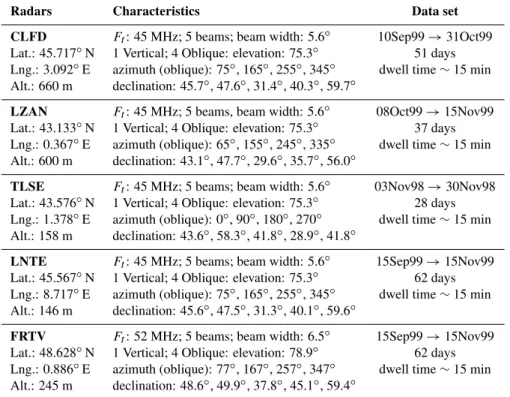
CLFD Ft: 45 MHz; 5 beams; beam width: 5.6◦ 10Sep99→31Oct99
Lat.: 45.717◦N 1 Vertical; 4 Oblique: elevation: 75.3◦ 51 days Lng.: 3.092◦E azimuth (oblique): 75◦, 165◦, 255◦, 345◦ dwell time∼15 min Alt.: 660 m declination: 45.7◦, 47.6◦, 31.4◦, 40.3◦, 59.7◦
LZAN Ft: 45 MHz; 5 beams, beam width: 5.6◦ 08Oct99→15Nov99
Lat.: 43.133◦N 1 Vertical; 4 Oblique: elevation: 75.3◦ 37 days Lng.: 0.367◦E azimuth (oblique): 65◦, 155◦, 245◦, 335◦ dwell time∼15 min Alt.: 600 m declination: 43.1◦, 47.7◦, 29.6◦, 35.7◦, 56.0◦
TLSE Ft: 45 MHz; 5 beams; beam width: 5.6◦ 03Nov98→30Nov98
Lat.: 43.576◦N 1 Vertical; 4 Oblique: elevation: 75.3◦ 28 days Lng.: 1.378◦E azimuth (oblique): 0◦, 90◦, 180◦, 270◦ dwell time∼15 min Alt.: 158 m declination: 43.6◦, 58.3◦, 41.8◦, 28.9◦, 41.8◦
LNTE Ft: 45 MHz; 5 beams; beam width: 5.6◦ 15Sep99→15Nov99
Lat.: 45.567◦N 1 Vertical; 4 Oblique: elevation: 75.3◦ 62 days Lng.: 8.717◦E azimuth (oblique): 75◦, 165◦, 255◦, 345◦ dwell time∼15 min Alt.: 146 m declination: 45.6◦, 47.5◦, 31.3◦, 40.1◦, 59.6◦
FRTV Ft: 52 MHz; 5 beams; beam width: 6.5◦ 15Sep99→15Nov99
Lat.: 48.628◦N 1 Vertical; 4 Oblique: elevation: 78.9◦ 62 days Lng.: 0.886◦E azimuth (oblique): 77◦, 167◦, 257◦, 347◦ dwell time∼15 min Alt.: 245 m declination: 48.6◦, 49.9◦, 37.8◦, 45.1◦, 59.4◦
map at 45 MHz which can be used for ST radars calibration at mid-latitude in the northern hemisphere. This map is de-duced from the composite of routine observations made by five VHF wind profilers.
2 Radar characteristics and data set
A standard ST radar used for wind profiling does not possess the beam steering versatility of a radio telescope. It is usu-ally limited to three fixed beam directions (one vertical and two orthogonal obliques), a number simply necessary to de-rive the three components of the wind under the assumption of horizontal homogeneity. To increase the reliability of the measurements, some of them are equipped with four oblique beams disposed by a 90 degree step in azimuth. To over-come this limitation, since our objective was to obtain from ST radars measurements a cosmic emission map with a cov-erage and resolution in declination as large as possible, the solution adopted was to combine observations from different pointing beam directions collected by ST radars at several geographical locations.
In the present study, measurements from five ST radars are used. Their relevant characteristics are presented in Table 1. More details on these five beam VHF radars, which are part of the French research ST network, have been given by Ney (1995). Four of them, at 45 MHz, are of the same type, using a coaxial-collinear antenna with a 5.6◦beam width. The last
one has a 52 MHz transmitter frequency and its antenna is made of a Yagi array providing a 6.5◦beam aperture. All of these radars make use of the same on-line and off-line data processing. The first three moments of the Doppler spectra and the noise level are recorded for 40 range gates, spaced along the radial by 375 m for the 45 MHz radars, and 500 m for the 52 MHZ radar. The observations used here (see Table 1) were collected in normal mode operation during the Mesoscale Alpine Program (MAP) in 1999 and in pre-MAP in 1998 (only for the TLSE radar). Depending on the radar, the data set corresponds to a number of days of continuous observations, ranging from 28 to 62. The mode of data col-lection is based on a repetitive cycle of measurements over the five beams with a duration of about 15 minutes.
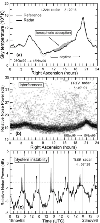
Figure 1a presents an example of the noise power observed during one week by one of the beams of the LZAN radar for a range gate positioned at an altitude of 14.5 km. Indeed, the measured cosmic noise power is not a function of the altitude of the measurements if the response function of the receiver and data processing is range independent. This figure clearly shows the diurnal (more precisely, sideral day) cycle of the noise, the power of which has a crest-to-crest amplitude of about 5 dB in that case. This confirms the dominant external origin of the noise observed at VHF band.
Fig. 1. Example of the temporal evolution of the noise power (dB uncalibrated) observed by one of the beams of the LZAN radar (δ= 35.66◦)(a)over a week versus universal time (UTC), and(b)as a function of right ascension.
and time of these measurements into declination (δ) and right ascension (α). Declination is the elevation of the beam above the equator and right ascension depends on the local sideral time, radar latitude, and pointing directions of the observa-tion. Right ascension values range from 0 to 24 hours and correspond to the 360◦diurnal rotation of the Earth. The
con-tinuous data collection of a fixed beam consists of a constant declination scan variable in right ascension. For the collec-tion time period of the observacollec-tions used here, we may con-sider the coordinatesδandαof any cosmic emission sources, fixed in an absolute referential, as constant with a very good accuracy. The secular variation of the direction of the Earth’s rotation axis, due to the phenomena of precession and nuta-tion, introduces slight modifications on theδ andαvalues which have to be taken into account when considering peri-ods of time greater than several tens years. The advantage of this equatorial coordinate system is that it permits the merg-ing into a right ascension day, the noise data collected at
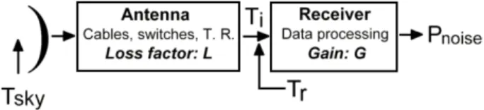
dif-Fig. 2.Block diagram of the receiving system (see text for detail).
ferent dates. This was done in Fig. 1b for the data presented in Fig. 1a. The original data sampling inαwas about 15 min, the accumulation of data over a week has increased this sam-pling by a factor of seven. This improvement inαsampling was one of the reasons to use a long period of observations.
3 Conversion of the radar noise to sky temperature
3.1 Basic equations
The theoretical background in radio-astronomy, radiometry, and system noise used here can be found, for instance, in the text books of Ulaby et al. (1981) and of Kuzmin and Salomonovich (1966), or in Hey et al. (1947). The block diagram of the radar receiving system is displayed in Fig. 2. The main assumptions made are that the cosmic radiation is unpolarized, it follows the black-body law, and the antenna is in radiative equilibrium with the surroundings. Note that linearly-polarized antenna collects half the incident unpolar-ized cosmic radiation power. The cosmic noise power gath-ered by a lossless antenna induces in the receiver system a thermal noise power equal tokTskyB; wherek is the Boltz-mann’s constant,B is the overall bandwidth of the receiving system, andTskyis the apparent cosmic emission temperature or sky temperature. The measured sky temperature results from the convolution between the beam illumination function and the sky radiation field. Consequently, the value ofTsky is dependent on the beam diagram, except when the cosmic radiation is uniform (or slowly varying) in the observed sky region. The width of the main beam has a smoothing effect on the measurements. More difficult to evaluate is the contri-bution due to the side lobes which can be important when the beam is directed toward the vicinity of a strong radio source. According to Milogradov-Turin and Smith (1973), Cassiopeia A, which is one of the strongest radio sources, in-duces a contribution of about 100 K at an angular distance of 15◦from the source. On an other hand, the cosmic emis-sion reflected by the ground and which enters the side lobes is negligible for our radars, with beams directed close to the zenith.
When taking into consideration losses and the other noise sources in the receiving system (see Fig. 2), the apparent sky temperatureTsky is related to the equivalent temperatureTi
at the receiver input by the following relationship:
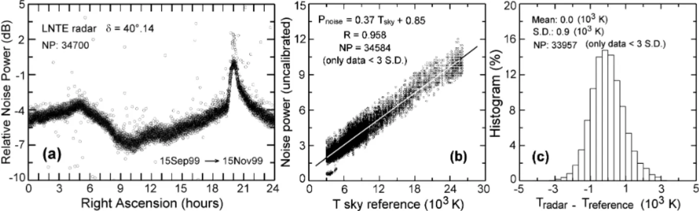
Fig. 3. Noise data collected between 15 September and 15 November 1999 by one of the beams (δ = 40.14◦) of the LNTE radar: (a) distribution of the relative noise power (dB) versus right ascension;(b)linear least square fit of the noise power (uncalibrated linear scale) as a function of the reference sky temperature (kK);(c)histogram of the difference between radar temperature and reference temperature. In (a) and (b) only data deviating by less than 3 standard deviations were used.
whereLis the loss factor (L≤1) of the modules ahead of the receiver (antenna, cables, switches. . . );Troomis the ambient temperature of the system (∼ 290 K);Tr is the addition of
the equivalent temperature, as seen at the receiver input of the non-thermal noise generated in the receiver (related to the noise figure) and of the processing data noise.
The noise powerPnoiseat the receiver output after data pro-cessing is equal toGTi, whereGis the gain of the receiver
and data processing. Using Eq. (1), one obtains the radar noise power to sky temperature conversion linear equation function of two instrumental constantsAandB:
Pnoise=ATsky+B (2)
In our case, the noise power corresponds to the noise level of the Doppler spectra obtained with the Hildebrand and Sekhon technique (1974). Since these data were acquired during routine operating conditions (i.e. when transmitting), in order to avoid leakage from strong returns (ground clutter, aircraft, etc.), we used the mean noise level measured at a high altitude between 13 and 15 km.
VHF band cosmic radiation is dominated by the non-ther-mal synchrotron emission which results from the interactions of ray electrons and the galactic magnetic field (Alvarez et al., 1996). As a consequence, the temperature of a sky region varies strongly with frequency. However, experience shows (see, for instance, Purton, 1966) that on average, sky tem-peraturesT1 andT2, respectively observed at two different frequenciesf1andf2, are related by the following relation-ship:
T1 T2
=
f
1 f2
−β
(3) whereβ is the spectral index which is assumed to be con-stant over a limited frequency band. From the comparison of observations made over the galaxy at 22 MHz and 408 MHz, Roger et al. (1999) foundβvalues ranging from 2.4 to 2.55.
In the same way, Purton (1966) obtained an interval of vari-ation of β between 2.0 and 2.5 from comparison of data acquired at 20 MHz and 240 MHz; Milogradov-Turin and Smith (1973), with 38 MHz and 404 MHz observations, re-port aβvariation between 2.48 and 2.58. We have used here, in particular for the conversion of the 52 MHZ radar obser-vations into 45 MHZ sky temperature, a mean spectral index of 2.5. Within the interval of variation ofβgiven above, this yields an uncertainty on the retrieved temperature of about 100 K, which corresponds to a relative error less than 3%. 3.2 Calibration of the radars
In a first step, it is necessary to calibrate the radars, i. e. to re-trieve theAandBconstants for each beam in order to access to the sky temperature. The calibrating method adopted was to relate the noise power measured by the radar to the sky temperature provided by a reference temperature map for the (δ, α) coordinates of the considered radar data. Equation (2) is then solved for the parametersAandB in a linear least square sense, using a long series of measurements. This pro-cedure was applied independently to each beam.
of 4◦ and 10 min, respectively. Unfortunately, only a
pa-per version of this map, presented as tempa-perature contours in equatorial coordinates, was available. This map was digi-tized, and the temperature and right ascension at the intersec-tion points of temperature contours and constant declinaintersec-tion lines, corresponding to those radar beams, were retained. On average, the data sampling of the map in the right ascension was 15 min. A slight correction was applied on the equato-rial coordinates of these reference data, acquired in 1967, to account for the effect of nutation and precession of the Earth rotation axis. No correction has been made to account for the small difference (∼2◦) between the beam apertures of the ST radars and that of the radio telescope. Finally, Eq. (3) was used with a spectral index of 2.5 to translate the 38 MHZ sky temperature into the sky temperature expected at the radar frequencies used.
A typical example of radar calibration and sky tempera-ture retrieval is presented in Figs. 3 and 4 for one of the beams (δ =40.14◦) of the LNTE radar. Figure 3a displays the distribution as a function of the right ascension of the 34700 noise power data collected continuously during two months. The linear least square fit of the radar noise data, as a function of the reference temperature, used to retrieve the calibration constants AandB (see Eq. 2), is shown in Fig. 3b. This adjustment has a very good correlation coeffi-cient of 0.96. OnceAandBare known, the radar noise power is expressed in terms of sky temperature, using Eq. (2). Fig-ure 3c presents the histogram of the difference between the retrieved radar sky temperature and the reference sky temper-ature. Note that in Figs. 3b and 3c, data deviating more than three standard deviations from the linear fit were discarded to avoid using the spurious data apparent in Fig. 3a. This procedure concerned less than 1% of the data which were not used in the final adjustment. On average, the temperature difference is null (a result expected with a least square fit). The standard deviation of this distribution has a value about 900 K. The data scattering, which can be seen in Fig. 3a, has indeed multiple potential sources: system instability, inter-ference, ionospheric absorption (these three sources of dis-turbance will be discussed in the next section), error in the reference map itself or during its digitization, a difference in beam resolutions (primarily important in sky regions with strong temperature extremum), natural variability of the sky brightness (Hey et al., 1947), etc.
In order to reduce the statistical uncertainty (or bias) of the measured temperature, a data smoothing in the right ascen-sion was performed, indeed at the expense of the resolution in theα coordinate. The method adopted was to take the temperature value resulting from a linear least square fit, ap-plied on the running interval inαof 20 min. Usually more than 50 data were involved in this smoothing. Once again, data deviating by more than three standard deviations were removed in the final adjustment. The temporal lag selected has an equivalent angular value of about 5◦, and thus, it is close to the radars beam width.
Figure 4a presents the resulting radar-temperature distri-bution as a function of right ascension, along with the
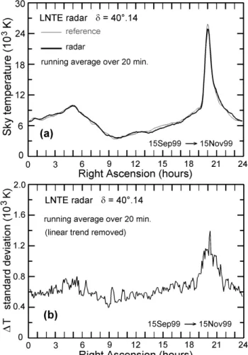
ref-Fig. 4. For the same data presented in Fig. 3: (a)comparison be-tween the sky temperature given by the reference sky survey and that deduced, after smoothing, from the radar power noise measure-ments as a function of right ascension; (b) standard deviation of the temperature derived from the radar data calculated on a running interval of 20 min in right ascension.
erence sky temperature curve. For the selected declination, sky temperature varies between 4 kK and 25 kK. In compari-son, the internal system noise temperature,Tr, is of the order
of 500 K. We may note the tight concordance between both curves which are nearly coincident. One may conclude, in particular, that the 2◦difference in beam resolution between
known, it is possible to deduce the gainGand the loss factor Lof the receiving system. From Eqs. (1) and (2), we obtain the following system of two equations with two unknowns: A=GL
B=G{(1−L)Troom+Tr} (4)
To resolve (4) forGandL, it is necessary to have an ac-curate estimate of the receiving and data processing noise temperature Tr. Experience has shown that this resolution
was very sensitive to the choice of Tr, and variations less
than 100 K in this temperature produced unrealisticL and Gvalues. Consequently, this straightforward approach, used by several authors quoted in the introduction, is not recom-mended. A better solution is to measure the system gain with a calibrated noise source; this can be easily done. Then, with an accurate estimate of G, the loss factor L, which is the more difficult radar parameter to verify, can be derived di-rectly fromA(see Eq. 4).
4 The results
4.1 Main difficulties
The observations of the 25 beams of the data set were pro-cessed, as explained in the preceding section. During this processing, three main problems were encountered: iono-spheric absorption, interference, and system instability. As mentioned earlier, the problem of strong echoes (ground clut-ter, aircraft, etc.) spreading over the Doppler spectra was avoided by using noise data collected at high altitude range gates.
Ionospheric absorption is a well-known phenomena which affects cosmic radiation when crossing the upper level of the atmosphere above the 100 km altitude (primarily, the D and E ionospheric layer are concerned). Ionospheric attenuation has a time scale from a few minutes up to several hours (Al-varez et al., 1997), and affects more low frequency radiation and data acquired at low elevation angles. Ionospheric opac-ity is first controlled by solar activopac-ity (linked to the solar spot number), so that nighttime observations are practically free from absorption (Milogradov-Turin and Smith, 1973). Ac-cording to Lamy et al. (1991), the attenuation can reach 2 dB at 45 MHz, during periods of strong solar activity. It is possi-ble to correct this effect if riometre measurements are avail-able (Milogradov-Turin and Smith, 1973). Figure 5a presents a clear example of the ionospheric disturbance observed in a beam (δ = 29.6◦) of the LZAN radar. Observations in the daytime were collected approximately within the right ascension interval between 12 and 18 hours. Inside this re-gion (hatched area), there is a temperature deficit reaching 1000 K, corresponding to a relative temperature error about
earlier).
Receivers working at low radio frequencies are particu-larly sensitive to natural interference or interference arising from human activities, such as lightning or radio emissions, which can propagate over long distances. Usually, these sig-nals, which increase the noise level at the expense of radar sensitivity, are sporadic, but occasionally, they can last for hours. The beam of the FRTV radar at the 49.91◦ declina-tion, the observations of which are plotted in Fig. 5b, was the most polluted beam of the data set. It is thought that the probable source of these interference are electric discharges from a high power line passing in the vicinity of the radar entering the antenna through a low-angled lobe. As it can be seen in this figure, the electric pollution can increase the noise level by 10 dB or more. The data processing based on a long series of observations enabled one to reject these spurious noise measurements and to retrieve a consistent sky temperature even in the strongly contaminated case.
For various reasons, like other instruments, a radar receiver system (including on-line data processing) may present dysfunction that could induce, for instance, a loss of sensitivity, noise generation, or receiver gain variation. The only solution is to check the data and reject them (if no correction is possible) when receiver system instability is suspected. In a first step, we tested the data on the basis that the mean noise power, taken over a sideral day, is nearly constant. Suspected periods were then checked visually and possibly rejected from the temperature retrieval. Figure 5c presents a case of receiver system instability, observed in the noise power time series of the TLSE radar beam at 58.28◦ declination. In that case, during the three last days of the series, there was a progressive diminution with time of the crest-to-crest amplitude of the noise power, along with an in-crease of its mean value.This was attributed to a dysfunction of the transmitter-receiver switch. This example shows the utility of the cosmic emission to control system performance. 4.2 Consistency between the different
radars measurements
Fig. 5. Example of the main difficulties encountered in the radar data processing: (a) ionospheric absorption during daytime ob-served in LZAN radar data (δ=29.6◦) when compared to the ref-erence temperature;(b)interferences on the most polluted beam of the data set (FRTV radar,δ=49.9◦);(c)receiving system instabil-ity characterized here by the decrease with time of the crest-to-crest amplitude of the noise power (TLSE radar,δ=58.3◦).
the LNTE and CLFD radar, respectively. The declination of these beams differs by 0.15◦. The agreement between both curves can be considered as very good, since the maximum
difference in temperature is less than about 300 K. This ac-curacy is sufficient for the purpose of radar calibration. More instructive is the comparison presented in Fig. 6b, which con-cerns data collected by the LNTE and FRTV radar differing both by the transmitted frequency and beam aperture. The difference in declination of the two compared beams is 0.22◦. Note that the sky temperature at 52 MHz of the FRTV radar was converted with Eq. (3) into a 45 MHZ equivalent tem-perature. This figure shows that in the period between 0 to 18 hours, the concordance between the radar’s tempera-tures is as good as in the preceding example. After 18 hours and up to 24 hours, the presence of a strong radio source induces notable discrepancies that can be attributed largely to the difference in the beam diagram of the radars. In par-ticular, the width of the peak centered about 2330 is larger for the FRTV radar which possesses the largest beam width (1◦ more). For this particular radar, we can also note that the peak is stronger, denoting that its beam is directed closer toward the center of the radio source.
4.3 The 45 MHZ sky temperature map
For the composition of the map, 16 beams out of 25 were re-tained. This selection was made on the basis of a data qual-ity control. Some of them where discarded since they were redundant with other beams which had very close declina-tions. This was the case, in particular, for all the beams of the CLFD and LNTE radars (see Table 1). In such a case of redundancy the best beam was selected. The declinations of the 16 beams retained for the map are (see Table 1 for the radar and beam correspondence): 28.9◦, 29.6◦, 31.4◦, 35.7◦, 37.8◦, 40.3◦, 41.8◦, 43.1◦, 45.6◦, 47.5◦, 48.6◦, 49.9◦, 56.0◦, 58.3◦, 59.4◦, 59.7◦.
On average, the sampling in declination is about 2◦, ex-cept within the intervals (31.4◦– 35.7◦) and (49.9◦– 56.0◦), where it reaches 4.3◦and 6.1◦, respectively. The temperature measurement covers the 24 hours of the right ascension co-ordinate. As a result of the smoothing realized during data processing, the resolution in right ascension is 20 min, or equivalently 5◦. These data were linearly interpolated into a regular equatorial coordinate grid. The interpolated tempera-ture map covers the sky region limited in declination between 30◦and 60◦(north), and 24 hours of right ascension.
Fig. 6.Comparison of the distribution of the sky temperature (kK) as a function of right ascension for pairs of beams with nearly the same declination angle: (a)LNTE radar (δ= 31.27◦) and CLFD radar (δ=31.42◦) data;(b)LNTE radar (δ =59.58◦) and FRTV radar (δ=59.36◦) data.
5 Summary and conclusion
The objective of this preliminary study was to assess the ca-pability of ST radar for astronomical survey, and to obtain a map of sky temperature at VHF band for radar calibration and monitoring. The originality of the work was to use data collected by an ensemble of five VHF ST radars during rou-tine mode meteorological operation. The use of long and continuous periods of observation allowed us to reach a fine right ascension resolution, with low temperature uncertainty, and to eliminate, with thresholding, spurious data due to var-ious sources of interference. The temperature map obtained for 45 MHz covers the sky region limited in declination be-tween 30◦and 60◦(north) and 24 hours of right ascension. The sampling in declination is over most of the map of about 2◦, and the right ascension resolution is 20 minutes.
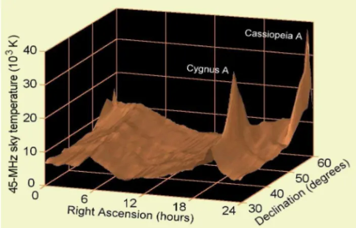
Temper-Fig. 7. Sky temperature map at 45 MHz, versus right ascension and declination, deduced from the observations of the five VHF ST radars. The two main peaks in temperature correspond to the emis-sion of the radio sources Cygnus A and Cassiopeia A, respectively.
ature uncertainty is about 600 K, which corresponds to a rel-ative error of 10% when considering a mean sky temperature of 6000 K. This accuracy is sufficient for the purpose of radar calibration. This map can be used for ST radar calibration at mid-latitude in the northern hemisphere. In the observed part of the sky, the galactic temperature varies between 4000 K and 36000 K and largely dominates the internal receiver sys-tem noise of the order of 500 K. Since sky emission is the main factor of the radar sensitivity at VHF band, a sky tem-perature map can serve to optimize the selection of the beam pointing direction for which the contribution of the sky noise is as low as possible during the day. This work is a first step, and the present map coverage will be extended in declination when other ST radar observations are available.
Acknowledgements. The French ST network is supported by INSU/ CNRS and M´et´eo-France.
Topical Editor J.-P. Duvel thanks R. Vincent and W. Singer for their help in evaluating this paper.
References
Alvarez, H., Aparici, J., May, J., and Olmos, F., A 45-MHz con-tinuum survey of the southern hemisphere, Astron. Astrophys. Suppl., 124, 315–328, 1997.
Baldwin, J. E., A survey of the integrated radio emission at a Wave-length of 3.7 m, Mon. Not. Roy. Astron. Soc., 115, 684–689, 1955.
Balsley B. B. and Gage, K. S., On the use of radars for operational wind profiling, Bull. Amer. Meteor. Soc., 63, 1009–1018, 1982. Brown, P., Hocking, W. K., Jones, J., and Rendel, J.,
Observa-tions of the Geminids and Quadrantids using a Stratosphere-Troposphere radar, Mon. Not. Roy. Astron. Soc., 295, 847–859, 1998.
Clark, W. L., Green, J. L., and Warnock, J. M., Monitoring VHF radar system performance using cosmic noise, Handbook for Middle Atmospheric Program, 28, 593–596, 1989.
Czechowsky, P., Schmidt, G., and Ruster, R., The mobile SOUSY-Doppler radar; technical design and first results, Handbook for Middle Atmospheric Program, 9, 433–446, 1983.
Gage, K. S. and Balsley, B. B., Doppler radar probing of the clear atmosphere, Bull. Amer. Meteor. Soc., 59, 1074–1093, 1978. Gage, K. S. and Green, J. L., Evidence for specular reflection from
monostatic VHF radar observations of the stratosphere, Radio Sci., 13, 991–1001, 1978.
Hey, J. S., Parsons, S. J., and Phillips, J. W., An investigation of galactic radiation in the radio spectrum, Proc. Roy. Soc., 192, 425–445, 1947.
Hildebrand, P. H. and Sekhon, R. S., Objective determination of the noise level in Doppler spectra, J. Atmos. Sci, 13, 808–811, 1974. Hocking, W. K. and Lawry, K., Radar measurements of atmospheric turbulence intensities by both Cn2 and spectral width methods, 4th Workshop on Technical and Scientific Aspects of MST radar, Handbook for MAP, 28, 242–247, 1989.
Hocking, W. K., Measurement of turbulent energy dissipation rates in the middle atmosphere by radar techniques: a review, Radio Sci., 20, 1403–1422, 1985.
Hooper, D. and Thomas, L., Aspect sensitivity of VHF scatterers in the troposphere and stratosphere from comparisons of powers in off-vertical beams, J. Atmos. Terr. Phys., 57, 655–663, 1995. Kuzmin, A. D. and Salomonovich, A. E., Radioastronomical
meth-ods of antenna measurements, Academic Press, 1966.
Lamy, B., Crochet, M., and Dalaudier, F., Calibration of ST radars using cosmic noise evolution: application to radar PROVENCE at 45 MHz, 5th Workshop on Technical and Scientific Aspects of MST Radar, STEP Handbook, 397–402, 1991.
Landecker, T. L. and Wielebinski, R., The galactic metre wave ra-diation: a two-frequency survey between declinations +25◦and
−25◦and the preparation of the map of the whole sky, Aust. J. Phys. Astrophys. Suppl., 16, 1–30, 1970.
Larsen, M. F. and R¨ottger, J., VHF and UHF Doppler radars as tools for synoptic research, Bull. Amer. Meteor. Soc., 63, 996–1008, 1982.
Milogradov-Turin, J. and Smith, F. G, A survey of the radio back-ground at 38 MHz, Mon. Not. R. astr. Soc., 161, 269–279, 1973. Ney, R., French INSU-METEO research ST radar network: geo-graphical and technical characteristics, 7th Workshop on Tech-nical and Scientific Aspects of MST Radar, STEP Handbook, 461–464, 1995.
Purton, C. R., The spectrum of the galactic radio emission, Mon. Not. Roy. Astron. Soc., 133, 463–474, 1966.
Riddle, A. C., Use of the sun to determine pointing of ST radar beams, Handbook for MAP, 20, 410–413, 1986.
Roger, R. S., Costain, C. H., Landecker, T. L., and Swerdlyk, C. M., The radio emission from the galaxy at 22 MHz, Astron. Astro-phys. Suppl., 137, 7–19, 1999.
Ulaby, F. T., Moore, R. K., and Fung, A. K., Microwave remote sensing active and passive, Addison-Wesley, vol. 1, 1981. Watanabe, J.-I., Nakamura, T., Tsutsumi, M., and Tsuda, T., Radar
observation of the strong activity of a Perseid meteor shower in 1991, Publ. Astron. Soc. Japan, 44, 677–685, 1992.
Werner, G., Bracewell, R. N., Deuter, J. H., and Rutherford, J. S., The sun as a test source for boresight calibration of mi-crowave antennas, IEE Trans. Antennas Propagat., AP-19, 606– 612, 1971.
Whiton, R. C., Smith, P. L., and Harbuck, A. C., Calibration of weather radar systems using the sun as radio source, Proc. 17th Radar Conf., Amer. Met. Soc., 60–65, 1978.