www.hydrol-earth-syst-sci.net/15/3077/2011/ doi:10.5194/hess-15-3077-2011
© Author(s) 2011. CC Attribution 3.0 License.
Earth System
Sciences
Forest cover influence on regional flood frequency assessment
in Mediterranean catchments
F. Preti1, G. Forzieri2, and G. B. Chirico3
1Dipartimento di Economia, Ingegneria, Scienze e Tecnologie Agrarie e Forestali, Sezione di Ingegneria dei Biosistemi Agrari e Forestali, University of Florence, Florence, Italy
2Dipartimento di Scienze della Terra, formerly at Dipartimento di Ingegneria Civile e Ambientale, University of Florence, Florence, Italy
3Dipartimento di Ingegneria Agraria e Agronomia del Territorio, University of Napoli Federico II, Napoli, Italy Received: 28 April 2011 – Published in Hydrol. Earth Syst. Sci. Discuss.: 16 May 2011
Revised: 15 August 2011 – Accepted: 12 September 2011 – Published: 7 October 2011
Abstract. The paper aims at evaluating to what extent the forest cover can explain the component of runoff coefficient as defined in a regional flood frequency analysis based on the application of the rational formula coupled with a re-gional model of the annual maximum rainfall depths. The analysis is addressed to evaluate the component of the runoff coefficient which cannot be captured by the catchment lithol-ogy alone. Data mining is performed on 75 catchments dis-tributed from South to Central Italy. Cluster and correla-tion structure analyses are conducted for distinguishing for-est cover effects within catchments characterized by hydro-morphological similarities. We propose to improve the pre-diction of the runoff coefficient by a linear regression model, exploiting the ratio of the forest cover to the catchment crit-ical rainfall depth as dependent variable. The proposed re-gression enables a significant bias correction of the runoff coefficient, particularly for those small mountainous catch-ments, characterised by larger forest cover fraction and lower critical rainfall depth.
1 Introduction
Flood peak assessment is fundamental for planning and de-sign structural and non-structural flood risk mitigation ac-tions. This is achieved by flood frequency analysis, which aims at estimating the probability distributions of flood peaks, so that the flood magnitude for any design return period can be easily determined. A direct assessment of
Correspondence to:F. Preti ([email protected])
for estimating the index flood at ungauged sites. Many in-direct methods are based on multiregression models linking the index flood to a selected set of catchment descriptors (e.g. Kjeldsen and Jones, 2010), representing morphologi-cal, climatic and land use catchment features. These regres-sion methods take generally little consideration of the phys-ical phenomena underlying the transformation of rainfall in runoff and of the dominant flood generating mechanisms, al-though more recent studies evidenced that flood generating mechanisms can be relevant in flood regional analysis (Iaco-bellis and Fiorentino, 2000; Mertz and Bl¨oschl, 2003). Other indirect methods provide an estimate of the flood index based on a conceptual description of the hydrological response of the basin to intense rainfall events. Within the flood assess-ment procedures employed in Italy, an indirect estimation method largely applied is based on a conceptual model struc-tured according to the well-known rational formula (Rossi and Villani, 1992). Other conceptual approaches have been also proposed, based on an analytical derivation of the prob-ability distribution of floods (e.g. Becciu et al., 1993; Brath et al., 2001; Bocchiola et al., 2003). The index flood esti-mation method based on the rational formula implicitly as-sumes that the average value of the annual maximum peak discharges is related to the average value of the annual max-imum rainfall depth within a critical time interval, which is assumed equal to a characteristic time scale of the catchment response. A key parameter is the runoff coefficient, which conceptually represents the fraction of the total rainfall con-tributing to the flood peak response. Runoff coefficient val-ues are derived by regional models with respect to selected catchment descriptors that can be easily distinguished at re-gional scale. A general tendency is to employ the catchment lithology as principal catchment descriptor of the runoff co-efficient, while assuming negligible the additional informa-tion attached to the land-cover patterns for the assessment of flood extreme values, at least in rural catchments (e.g. Iaco-bellis and Fiorentino, 2000; Brath et al., 2001).
As result of the index flood approach, the flood frequency curves within homogenous regions are shifted according to the value of the index flood, while keeping the same shape.
Another regionalisation procedure is based on the use of rainfall-runoff models (e.g. Maidment, 1993). In this case, annual maximum rainfall depths of various durations are treated through a regionalisation procedure, such as the index value approach, whereas the discharge with an as-signed return period is estimated by applying a rainfall-runoff model. This second type of regionalization procedure based on rainfall-runoff models is more effective in repre-senting the flood frequency distribution in regions that, al-though being homogeneous in terms of annual maximum rainfall depths, include catchments with significantly dif-ferent flood frequency curves as result of difdif-ferent rainfall runoff processes controlling the flood response. In engi-neering applications, the most widely used rainfall-runoff model is still the rational formula, often applying the runoff
coefficient as function of the return period (Schaake et al., 1967; French et al., 1974; Pilgrim, 1989; Cannarozzo et al., 1995). In this case, the runoff coefficient does not simply represent a runoff rainfall ratio, rather it assumes the role of a probabilistic factor controlling not only the position but also the slope and the curvature of the flood frequency curve, by means of a (generally, non-linear) transformation of the catchment rainfall frequency curve for a catchment charac-teristic time scale. In some studies, the dependency of the runoff coefficient from the return period has been explored by a specific probabilistic model, considering the runoff co-efficient independent from the rainfall depth (Gottschalck and Weingartner, 1998; Franchini et al., 2005).
The dependency of the runoff coefficient with the return period is consistent with the consideration that, particularly in rural catchments, there is not a perfect correspondence be-tween annual maximum peak discharges and annual maxi-mum rainfall depths (e.g. Hiemstra and Reich, 1967; Frchini et al., 2000; Haschemi et al., 2000). The maximum an-nual flood peak is in fact controlled by catchment antecedent conditions and thus can be also generated by rainfall events with catchment average depth even below the annual max-imum. This aspect cannot be represented with a constant runoff coefficient, as it occurs in traditional applications of the rational formula.
Provided that vegetation patterns can have a significant in-fluence on the catchment antecedent conditions as well as on other rainfall runoff processes in rural catchments, in this study we explore to what extent forest cover can be employed to predict the runoff coefficient, in the framework of a re-gional flood frequency analysis based on the rational formula coupled with a regional analysis of annual maximum rainfall depths.
The paper is structured as follows: the following sec-tion presents the regional flood frequency analysis; the third section illustrates the available data set; the fourth section explores the dependency of the runoff coefficient from the forest cover; in the fifth section we present a new regres-sion model of the runoff coefficient accounting for the forest cover; the sixth section is devoted to the discussion and the last section to the conclusions.
2 Regional flood frequency analysis based on the rational formula
The flood peak for a given return periodT,QT, can be de-fined as follows:
QT = KQ,T µQ (1)
whereKQ,T is the dimensionless probabilistic growth factor of the floods for a return period equal toT andµQ is the index flood.
factor, controlling the slope and the curvature of the flood frequency distribution, is invariant within the homogenous region, while the index flood, controlling the position of the flood frequency distribution, is variable and can be predicted by catchment specific descriptors. A common approach for estimating the index flood µQ in Italian ungauged catch-ments is based on a conceptual model structured according to the well-known rational formula:
µQ =φ A
µ[hA (tc)]
tc
(2) whereAis the catchment area, whileφis the runoff coeffi-cient for the index flood (0< φ≤1), i.e. the ratio of the mean flood runoff to the mean rainfall depth, assumed to be inde-pendent of rainfall intensity and duration; µ[hA(tc)]is the catchment areal rainfall depth within a critical durationtc, obtained by multiplying the point depth-duration-frequency curveµ[h(tc)](referred to the centre of the storm) with the area reduction factorκA, which is expressed as function of the catchment area and the critical durationtc (e.g. Brath et al., 2001).
The runoff coefficientφis estimated by regression models against selected catchment descriptors, with invariant param-eters within homogenous regions. These regional models are calibrated with data of gauged catchments, where runoff co-efficients (φobs) are computed by inversion of Eq. (2) with index flood values (µˆQ) assessed by arithmetic average of the annual flood peak experimental values:
φobs = ˆ
µQtc
µ[hA (tc)]A
. (3)
It is important to observe thatφconceptually describes both the fraction of rainfall volume retained by the soil and the vegetation (i.e. the transformation of the total rainfall in net rainfall as result of processes such as infiltration, canopy in-terception and surface detention), and the dampening effect of the catchment, which implies the reduction of the flood peak as compared to the net rainfall intensity (for example, if the basin is modeled as a linear reservoir with lag time equal totL, the flood peak reduction with respect to a constant rain-fall intensity is equal to 1−e−tc/tL).
As anticipated above, regional regression models of the runoff coefficient generally exploit only classes of catchment lithology as predictor variables. At regional scale, the litho-logical features of the catchments can be grouped accord-ing to different classes correspondaccord-ing to different degrees of permeability, such as (e.g. Fiorentino and Iacobellis, 2001): (1) highly permeable lithoid complexes constituted by sed-iments and rocks with porosity based permeability, rocks with fissure-based permeability, and those having a mixed permeability; (2) lithoid complexes with medium permeabil-ity constituted by permeable lithologies which outcrop on a steep surface or lithologies more or less fractured and filled by clayey material; and (3) impermeable lithoid complexes represented by clayey formations.
In the case of a regional flood frequency analysis coupling a regional model of the annual maximum rainfall depths and a rainfall-runoff model structured according to the rational formula, the flood peakQT for a given return period is esti-mated in ungauged catchments as follows:
QT = CT A
hA,T (tc)
tc =
CT KR,T A
µ[hA (tc)]
tc
(4) wherehA,T (tc)is the catchment areal rainfall with return pe-riodT, expressed as the product of the dimensionless proba-bilistic growth factor of the rainfall for a return period equal toT,KR,T, and the index valueµ[hA(tc)];CT is the runoff coefficient for a return period equal to T. Sample values of the runoff coefficient (CT ,obs) can be derived by inverting Eq. (4) applied to gauged catchments, where enough data are available for a direct assessment of the flood frequency distri-bution, defined byKQ,T andµˆQ. In particular, by combing Eqs. (1) and (4),CT ,obscan be expressed as follows:
CT ,obs =
ˆ µQtc
µ[hA(tc)]A
KQ,T KR,T
= φobs
KQ,T KR,T
. (5) Equation (5) shows thatCT is the product of two terms: the first is the runoff coefficient for the index flood; the second term is the ratio of the rainfall and flow probabilistic growth factors, i.e. it describes the transformation of the slope and curvature of the flood frequency distribution with respect to the annual maximum rainfall depth frequency distribution.
It is important to note thatCT is not restricted to those val-ues commonly attached to the traditional runoff coefficient asφ(0< φ≤1). According to Eq. (5),CT is a probabilistic factor, which in principle could assume values even greater than 1, as for example when the flood frequency curves ex-hibit a significantly greater curvature than the corresponding rainfall frequency curves (Franchini et al., 2005).
We callCLthe value of theφcoefficient estimated by re-gression models accounting for the catchment lithology only, calibrated at regional scale against the observed valuesφobs, as defined by Eq. (3). Then we express the component of the runoff coefficient not explained by the cathment lithology, for a generic return periodT, as follows:
1CT =
CT ,obs −CL
CT ,obs
. (6)
In the hypothesis thatφ is fully described by CL,1CT is only representative of the ratio of the rainfall and flow prob-abilistic growth factors.
3 Available data
catchments in Central and Southern Italy (Fig. 1): 34 catch-ments in Toscana, 17 in Lazio, 12 in Campania and 12 in Sicilia. These catchments belong to different rainfall and flood homogeneous regions, as delineated by regional fre-quency analyses. The climate is quite variable among the study catchments, owing to significant variation in the geo-graphic latitude. Sicilia is characterized by semiarid or dry subhumid climate, with mild, not very rainy winters, and warm and very dry summers. As one proceeds north (toward Campania, Lazio and Toscana), the climate turns to wet sub-humid and sub-humid, with a marked seasonality, characterized by very wet winters and dry summers.
The following hydro-morphological parameters have been collected from the available reports and papers (Birtone et al., 2008; Calenda et al., 2003; Di Stefano and Ferro, 2007; Rasulo et al., 2009; Regione Toscana, 2007):
– catchment area (A);
– catchment mean elevation (Zm) above catchment outlet;
– catchment critical storm duration, assumed equal to the concentration time (tc);
– catchment critical rainfall depth (hc) for a reference re-turn period of 20 years (hc=hA,T=20(tc));
– catchment fraction with highly permeable lithoid com-plexes (Sp);
– catchment fraction with forest cover (Sb);
– runoff coefficient of the index flood estimated by re-gional regression models accounting for the catchment lithology only (CL);
– observed values of the runoff coefficient, defined ac-cording to Eq. (5), for a reference return period of 20 years (Cobs=CT=20,obs).
We selected the catchment mean elevation (Zm) above catch-ment outlet as this is one of the three catchcatch-ment descriptors appearing in theGiandottiempirical formula employed for computing the catchment concentration time (e.g. Brath et al., 2001):
tc =
4√A+1.5L
0.8√Zm
(7) whereL(km) is the main river length.
CL is computed by multiregression equations against the catchment fractions with different degree of permeability, as derived from lithological maps at regional scale. Within the sample catchment set,Spexplains almost 80 % of the overall variability ofCLamong the examined catchments. For this reason we selected onlySpamong the parameters describing the lithological classes within the study catchments.
The forest cover fractionSb is evaluated as the average value from land use maps of the same period analysed for
Fig. 1.Italian regions where the outlets of the 75 study catchments are located; from South (dark grey) to North: Sicilia (12 catch-ments), Campania (12 catchcatch-ments), Lazio (17 catchcatch-ments), Toscana (34 catchments).
assessing the observed runoff coefficient, mostly collected from 1960 and 1990 (e.g. Ferro and Porto, 2006). The spon-taneous vegetation and land cover in Central and Southern Italy is quite consistent with climatic features and morpho-logical characteristics of the territory. Arid and semiarid zones are characterized by scarce vegetation, which grad-ually turns into subhumid Mediterranean undergrowth and pasture land, to finally reach the mountain woods of humid and hyperhumid areas (Fiorentino and Iacobellis, 2001).
In the following section we examine the data set to dis-close the dependency of 1C=1CT=20 from the forest cover fraction and the selected set of hydro-morphological parameters.
4 Data mining
Fig. 2.Histograms of the hydro-morphological parameters: catchment extent (A); elevation above catchment outlet (Zm); concentration time (tc); maximum annual rainfall depth within a time interval equal totcand a return period of 20 years (hc); catchment fraction with highly permeable lithoid complexes (Sp).
Table 1. Mean (µ) and standard deviation (std) of the hydro-morphological variables for the examined catchments.
A Zm tc hc Sp CL Cobs
(km2) (m a.s.l.) (h) (mm) (%)
µ 712 383 9.2 76.5 25.5 0.57 0.49
std 1129 177 7.2 25.4 29.6 0.29 0.27
4.1 Preliminary data analysis
The following preliminary analyses have been conducted:
– histogram analysis;
– non-parametric correlation analysis of the hydro-morphological variables;
– dependence analysis of 1C from each of the hydro-morphological variables and the forest cover fraction. Histograms show the large variability of the hydro-morphological features of the examined catchments (see Ta-ble 1 and Fig. 2). A large number of catchments have an ex-tent smaller than 1000 km2and a surface fraction with high permeability (Sp) smaller than 20 %. The distributions ofA
andtcare very similar and exhibit a large skweness, while
hcdistribution is more uniform as direct consequence on the non-linearity of the rainfall depth-duration curve. Almost 50 % of the catchments are characterized by a concentration time smaller than 8 h: all 12 catchments in Sicily; 4 catch-ments in Campania; 2 in Lazio and 22 in Toscana. Only 10 catchments (13 %) have a concentration time larger than 18 h: 4 in Campania, 4 in Lazio and 2 in Toscana. The aver-ageCLis 0.57, with a standard deviation of 0.29, while the averageCobs is 0.49 with a standard deviation of 0.27 (see Table 1).
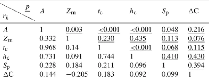
Table 2.Correlation analysis among the hydro-morphological vari-ables for the examined catchments: Spearman rank (rk) correlation in the lower triangular matrix; corresponding p-values (p) in upper triangular matrix.
❍ ❍
❍ ❍❍
rk
p
A Zm tc hc Sp 1C
A 1 0.003 <0.001 <0.001 0.048 0.216
Zm 0.332 1 0.230 0.435 0.113 0.076
tc 0.968 0.14 1 <0.001 0.068 0.115
hc 0.731 0.091 0.744 1 0.410 0.430
Sp 0.228 0.184 0.211 0.096 1 0.394
1C 0.144 −0.205 0.183 0.092 0.099 1
The correlation analysis has been performed through the Spearman rank instead of the standard Pearson coefficient to better capture possible non-linear regressions (Wilks, 1995). Many of the analyzed hydro-morphological variables ex-hibit significant cross-correlation (see p-values in Table 2), while none of these variables appears significantly correlated with1C. As expected, there is a significant positive corre-lation between A, tc, andhc. In fact, smaller catchments corresponds to lower order basins located in mountain areas, characterised by higher slope, smaller concentration time and smaller critical rainfall depth.
We also conducted an explanatory analysis among terns of variables1C−Y−Sb, whereY represents one of the se-lected hydro-morphological variablesA,Zm,tc,hc andSp, taken in turn. In Fig. 3, the contour maps represent the vari-ability of each hydro-morphological variable with respect to theSbvalues along the x-axis and the variable1C along the y-axis.
Fig. 3.Contour maps ofSbwith respect to1C for different hydro-morphological variables: catchment extent(A), elevation(B), concentra-tion time(C), reference rainfall intensity(D)and permeable lithoid fraction(E). White dots indicate the observed values.
4.2 Cluster analysis
The k-means method has been chosen in this study as a simple solution, characterized by short computation times, for the characterization of possible hydrological similari-ties (MacQueen, 1967). The method performs an unsuper-vised classification based on the frequency distribution of the hydro-morphological variables. Catchments are grouped ac-cording to the k-meanscluster analysis following two dif-ferent procedures: (i) clustering based on individual hydro-morphological variables, in order to assess the role of each parameter in theSb−1C relation; (ii) clustering including all parameters (hereafter indicated as HP case), to explore the effect of the reciprocal interaction among different pa-rameters in theSb−1C relation. Catchment clusters are in-dentified by maximizing the mean of the silhouette plot (Sh), which is a distance metric based on the squared of the Eu-clidean distance. Sh indicates the distance of each catch-ment value within a given cluster from the catchcatch-ment values belonging to other clusters and ranges from +1 to−1. Sh provides an indirect measure of the inter-cluster separability (Rousseeuw, 1987): +1 suggests a correct catchment cluster-ing, whereas−1 indicates a possible misclassification. Ex-amples of silhouette plots are depicted in Fig. 4.
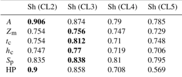
Table 3 shows the Sh for a number of clusters between 2 and 5, for each of the parameter examined and for the HP case. The values in bold indicate the Sh threshold values
Table 3.Sh values for different clustering levels. In bold Sh thresh-old value above which further clustering is not acceptable.
Sh (CL2) Sh (CL3) Sh (CL4) Sh (CL5)
A 0.906 0.874 0.79 0.785
Zm 0.754 0.756 0.747 0.729
tc 0.754 0.812 0.71 0.748
hc 0.747 0.77 0.719 0.706
Sp 0.835 0.838 0.81 0.795 HP 0.9 0.858 0.708 0.569
above which further clustering does not add much to the catchment classification. We identified 2 clusters for the catchment extentAand three clusters for each of the remain-ing 5 parameters. When we analyzed all parameters (HP), we selected 2 clusters.
Fig. 4.Example of silhouette plots for cluster analysis.
Table 4. Catchment clustering based on the analysis of single parameters. Statistics of the parameter values in each cluster: mean (µ), standard deviation (std), number of samples (n), and value ranges corresponding to the quantiles 0.05 and 0.95 (Min and Max, respectively).
CL1 CL2 CL3
µ std n Min Max µ std n Min Max µ std n Min Max
A 299.98 322.58 64 15.584 980 3114.4 1161.2 11 1921.1 5469.9 – – – – –
Zm 735.56 67.082 10 637 813 256 61.475 42 154.77 346.32 463.11 57.115 23 375.47 561.72
tc 3.858 1.571 40 1.515 6.47 11.965 2.611 25 8.597 16.776 23.616 4.173 10 18.65 31.416
hc 33.576 5.295 11 24.848 39.617 66.993 8.784 31 52.582 80.232 99.767 11.254 33 87.06 123.09
Sp 87.461 11.176 8 69.801 99.989 46.441 11.127 21 27.731 60.806 5.221 7.634 46 0.01 22.491
Table 5. Catchment clustering based on the analysis of the entire set of parameters (HP). Statistics of the parameter values in each cluster: mean (µ), standard deviation (std), number of samples (n), and value ranges corresponding to the quantiles 0.05 and 0.95 (Min and Max, respectively).
CL1 CL2
µ(CL1) std (CL1) n(CL1) Min Max µ(CL2) std (CL2) n(CL2) Min Max
HP (A) 854.57 1341.2 32 12.1 4014.2 607.25 944.94 43 31.28 3078.7 HP (Zm) 322.55 129.15 32 154.42 548.35 428.79 195.85 43 196.92 789.45 HP (tc) 10.103 7.967 32 1.409 27.699 8.519 6.57 43 1.872 24.472 HP (hc) 69.775 30.291 32 26.607 111.71 81.526 19.882 43 52.981 112.55 HP (Sp) 28.984 27.187 32 0.01 93.485 22.968 31.333 43 0.01 85.436
within each cluster is identified by the quantiles 0.05 and 0.95 of the corresponding sample distributions in each cluster. These ranges do not overlap when the clusters are identified by analyzing one parameter at a time, except for the clusters identified with the parameterAonly. When all parameter are considered in the clustering process (HP), the distinction of each cluster is more difficult, since value ranges overlap, as we might expect by examining the corresponding mean and std values (see Table 5).
4.3 Correlation structure
We calculated the Spearman’s rank correlation and the corre-sponding significance level (p-values) betweenSb−1C for each combination of parameters and for each cluster inden-tified (Table 6). Significant correlation occurs for the cluster with the largest number of samples for each fixed parameter. This suggests that for those clusters with a limited number of samples, the correlation might be underestimated. For the HP case no significant correlation has been identified.
Fig. 5.Sinfrepresents those (Sb,1C) couples which values of the corresponding hydro-morphological parameters are below its intra-cluster average. Ssuprepresents those (Sb, 1C) couples which values of the corresponding hydro-morphological parameters are above its intra-cluster average. Regression lines between1C and forest cover fraction for selected clusters of the study catchments: (i) including all (Sb, 1C) couples belonging to the examined cluster (LRtot); (ii) including onlySinfcouples (LRinf); (iii) including onlySsupcouples (LRsup).
Table 6.Spearman’s rank correlationSb−1C and corresponding p-values, within each cluster for a given parameter set. In bold those with p-values below 0.05.
Parameter rk p
Set CL1 CL2 CL3 CL1 CL2 CL3
A −0.36 −0.29 NaN 0.003 0.386 –
Zm 0.078 −0.233 −0.466 0.838 0.136 0.026 tc −0.285 −0.403 −0.066 0.074 0.046 0.864 hc −0.318 −0.636 −0.203 0.341 0.000 0.255 Sp 0.19 −0.271 −0.474 0.664 0.233 0.000 HP −0.052 −0.201 – 0.774 0.196 –
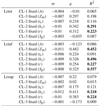
runoff coefficient which could be explained bySb. The good-ness of fit of the linear models are estimated by the coeffi-cient of determination (R2). The regression analysis is ap-plied to three different sets: (i) including all (Sb,1C) cou-ples belonging to the examined cluster (LRtot); (ii) including (Sb,1C) couples which values of the corresponding hydro-morphological parameters are below its intra-cluster average (LRinf); (iii) including (Sb,1C) couples which values of the corresponding hydro-morphological parameters are above its intra-cluster average (LRsup). Results are listed in Table 7. Figure 5 shows the computed regression lines for the selected clusters.
The possibility to explain1C withSbis highly variable, particularly in the case all catchments belonging to a clus-ter are included in the regression analysis (LRtot). Higher
R2 can be gathered if only those catchments in the lower range of the corresponding parameter values are included in the regression analysis (LRinf). The best fitting is obtained for LRinf within CL-3 fixed (Zm), CL-2 fixed (hc) and CL-3 fixed (Sp).
Table 7. Results of linear regression analysis: slope (m) and inter-cept (q) of the regression lines; coefficient of determination (R2).
m q R2
Lrtot CL-1 fixed (A) −0.004 −0.01 0.065 CL-3 fixed (Zm) −0.007 0.297 0.198 CL-2 fixed (tc) −0.007 0.218 0.116 CL-2 fixed (hc) −0.01 0.342 0.291 CL-3 fixed (r) −0.01 0.312 0.223 CL-3 fixed (Sp) −0.003 −0.035 0.087
Lrinf CL-1 fixed (A) −0.003 −0.123 0.086 CL-3 fixed (Zm) −0.011 0.482 0.452 CL-2 fixed (tc) −0.006 0.224 0.091 CL-2 fixed (hc) −0.009 0.326 0.496 CL-3 fixed (r) −0.009 0.254 0.227 CL-3 fixed (Sp) −0.008 0.325 0.557
Lrsup CL-1 fixed (A) −0.007 0.22 0.079 CL-3 fixed (Zm) −0.002 0.02 0.015 CL-2 fixed (tc) −0.007 0.175 0.121 CL-2 fixed (hc) −0.012 0.411 0.218 CL-3 fixed (r) −0.01 0.383 0.224 CL-3 fixed (Sp) −0.001 −0.173 0.009
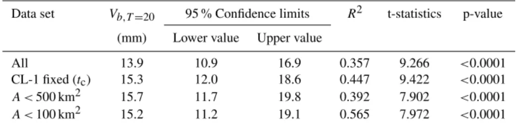
Table 8.Results of the regression analysis with four different catchment data sets: all catchments; catchments included in the cluster CL-1 fixed (tc); catchments with an areaA <500 km2; catchments with an areaA <100 km2.
Data set Vb,T=20 95 % Confidence limits R2 t-statistics p-value
(mm) Lower value Upper value
All 13.9 10.9 16.9 0.357 9.266 <0.0001 CL-1 fixed (tc) 15.3 12.0 18.6 0.447 9.422 <0.0001
A <500 km2 15.7 11.7 19.8 0.392 7.902 <0.0001
A <100 km2 15.2 11.2 19.1 0.565 7.972 <0.0001
These results suggest the possibility to explore new regres-sion models for predicting the runoff coefficientCT=20, ac-counting for the forest coverSb, at least within catchments classes which can be considered homogeneous with respect tohA,T=20(tc).
5 A new simple conceptual model for runoff coefficient assessment
Predicted values of the runoff coefficients from the catch-ment lithology (CL) are generally negatively biased with re-spect to the observed runoff coefficient Cobs. Moreover, the absolute difference Cobs−CL tends to be higher for catchments with smaller concentration time, as illustrated in Fig. 6. This suggests that there are larger margins for cor-recting the prediction of the runoff coefficients in catchments with smaller concentration time, which are generally those basins characterized by larger forest cover fractions, as these catchments are of lower order and higher slope, mostly lo-cated in mountainous areas.
Following the results of the previous cluster analysis, we explore the possibility to correct the biasCobs−CL with a runoff coefficientCT=20 expressed by a simple regression model of the forest coverSb scaled by the critical rainfall depthhA,T=20(tc):
CT=20 =CL −Vb,T=20
Sb hA,T=20 (tc)
. (8)
According to Eq. (8), the runoff coefficient estimated from the catchment lithology only (CL) is reduced by a factor
Vb,T=20 Sb/ hc, which conceptually could be interpreted as an additional abstraction loss of the total rainfall due to the storage capacity of the forested fraction of the catchment, with a specific volume equal toVb,T=20. Moreover,
recall-ing Eq. (5), the term[1−(Vb,T=20 Sb)/(hA,T=20 (tc) CL)] describes the ratioKQ,T=20/KR,T=20, if we assume thatCL represents the ratio between the corresponding index values. The optimal value Vb,T=20 can be assessed by least squares method applied to a linear regression model with the dimensionless ratioSb/ hA,T=20(tc)as independent variable
-0.50 0.00 0.50
0 5 10 15 20 25 30 35
tc [h] Co
b
s
C
L
Fig. 6.Differences betweenCobsandCLversus the catchment con-centration time.
and(CT=20−CL)as dependent variable, exploiting(Cobs−
CL)as sample data.
Figure 7a shows the fitted linear regression model with the corresponding scatter plot. The standardized residuals ap-pear normally distributed, as depicted in Fig. 7b and c. The optimalVb,T=20results equal to 13.9 mm, with a determina-tion coefficient (R2) equal to 0.357 (see Table 8). The null hypothesis of no linear correlation is rejected with a p-value below 0.0001. The 95 % confidence interval spans 6 mm around the expected value.
If we restrict the analysis to catchment clusters selected with respect totc as illustrated in the previous section, the prediction performance improves with small changes in the optimalVb,T=20. For example, as illustrated in Table 8, lim-iting the analysis to CL-1 fixed (tc), the optimalVb,T=20 is equal to 15.3 mm with aR2equal to 0.447.
The prediction performance also improves if we restrict the analysis to smaller catchments, still with slight changes in the predicted Vb,T=20 (see Table 8): for catchment ar-eas smaller than 500 km2, we get Vb,T=20= 15.7 mm and
R2= 0.392; for catchment areas smaller than 100 km2, we getVb,T=20= 15.2 mm andR2= 0.565.
(
)
( )
-0.4-0.3 -0.2 -0.1 0 0.1 0.2 0.3
0 0.005 0.01 0.015 0.02
Sb/hA,T=20 [1/mm]
C
T
=
2
0
-C
L
-3 -2 -1 0 1 2 3
0 0.005 0.01 0.015 0.02
Sb/hA,T=20 [1/mm]
s
ta
n
d
a
rd
iz
e
d
r
e
s
id
u
a
l
a) b) c)
Fig. 7. (a)Scatter plot and linear regression between (CT=20−CL) andSb/ hA,T=20 (tc); (b)scatter plot of standardized residuals; (c)frequency distribution of the standardized residuals and corresponding normal fit.
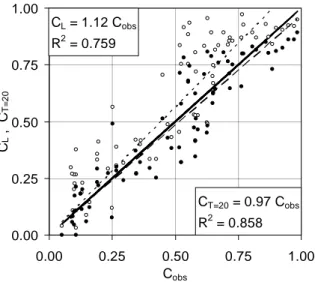
CT=20 = 0.97 Cobs
R2 = 0.858
CL = 1.12 Cobs
R2 = 0.759
0.00 0.25 0.50 0.75 1.00
0.00 0.25 0.50 0.75 1.00
Cobs
CL
,
CT
=
2
0
Fig. 8.Comparison between observed and predicted runoff coeffi-cients: open circles, (Cobs,CL); filled circles, (Cobs,CT=20). The dotted line is the linear regression betweenCobsand CL; the dashed line is the linear regression betweenCobsandCT. The linear regres-sions are compared to the continuous line, representing the perfect agreement.
performances are evaluated by computing the bias, the ab-solute bias (Abias) and the root mean square error (RMSE), as follows:
Bias = N P
i=1 erri N
Abias = N P
i=1 |erri|
N (9)
RMSE = v u u u t
N P
i=1
(erri)2 N
-0.50 0.00 0.50
0 5 10 15 20 25 30 35
tc [h] CT
=
2
0
C
L
Fig. 9. Differences betweenCT=20 andCLversus the catchment concentration time.
where N is the total number of catchment data and erri represents the deviation between the observed and the predicted runoff coefficients, erri= (Cobs−CT=20) or
erri= (Cobs−CL). As illustrated in Table 8, all three perfor-mance statistics indicate that there is an improvement of the predicted runoff coefficient withCT=20. The bias correction
is particularly high in catchments with higherSb/ hA,T (tc) ratios. Figure 9 shows how the (negative) bias correction tends to zero as the catchment concentration time increases. Higher catchment concentration time values correspond to higherSb/ hA,T (tc)ratios, which belong to small mountain-ous catchments, with higher slope and higher forest cover, which are characterized by small concentration time and small critical rainfall depth.
6 Discussion
within the hydrological cycle and in catchment response to small storms, does not mitigate significantly floods during extreme rainfall events (e.g. Calder, 2007; van Diijk and Keenan, 2007). This opinion is also prompted by influen-tial United Nation Policy documents (e.g. FAO and CIFOR, 2005; Hamilton, 2008), which confine the public perception to a misconception conceived by those who are not directly involved in studying hydrological extreme events, including environmentalists and conservation agencies. Experimen-tal studies show that forest cover reduces the annual catch-ment discharge as result of increased rainfall interception, increased transpiration and lower soil moisture regime dur-ing interstorm periods and higher permeability of forest soil (e.g. Bosch and Hewlett, 1982; Cornish, 1993; Rowe and Pearce, 1994; Stednick, 1996; Fahey and Jackson, 1997; Bruijnzeel, 2004). On the other hand, it is more difficult to assess the impact of forests on floods catchment response response to rainfalls with low frequency, due to lack of ex-perimental data for quantifying the effect of forests on the catchment response to rainfalls with low frequency (Nelson and Chomitz, 2007). Moreover, the effect of forest cover on flood peaks is difficult to be isolated, being the flood dis-charge influenced by other factors, such as initial catchment conditions, forestry and agricultural activities, road construc-tions, etc. (Moore and Wondzell, 2005).
Alila et al. (2009) pointed out that some contrasting con-clusions about the relation between forests and floods is the result of catchment paired studies, which do not account for the effect of forest cover on the non-linear dependency be-tween magnitude and frequency of floods. Alila et al. (2009) challenged decades of peer reviewed paired watershed study literature, arguing that the experimental design and statis-tical methods used in paired watershed studies have over-looked a fundamental part of the physics of the relation be-tween forests and floods, namely that forest affects not only the magnitude but most importantly the frequency of floods. Moreover, because of the strong non-linearity of the flood frequency distribution, small changes in the magnitude of extreme floods can translate into large changes in the cor-responding return periods (Alila et al., 2009, 2010).
Previous studies paid much attention to the effect of forest cover changes. In fact, forest patterns have been subjected to significant changes worldwide, with different trends, depend-ing specifically on local socio-economic and environmental factors. There are some areas of the world where forest cover has been reducing as results of logging and land claim for agriculture or urban infrastructures. Other areas, such as Mediterranean landscapes, forest patterns are experiencing a significant expansion in the last decades, as consequence of the abandonment of the agricultural lands in marginal ar-eas, mostly located in hilly and mountainous arar-eas, providing space for the natural development of forest (Mazzoleni et al., 2004).
It is important to point out that forest cover change is a source of non-stationarity and its effect on catchment
response cannot be analyzed in studies such as the present one. In fact, herein we explore the role of the forest cover on the runoff coefficient as defined in a regional flood fre-quency analysis, based on the application of the rational for-mula coupled with a regional model of the annual maximum rainfall depths, which inherently assumes that catchments are in stationary conditions.
Within this framework, the runoff coefficient looses its original meaning of output-input ratio of a rainfall-runoff model, as it occurs in the original interpretation of the ra-tional formula, while it assumes the role of a probabilistic factor, which describes the ratio of the flood peak to the max-imum annual rainfall depth for a given return period, i.e. the ratio between two random variables paired by the same fre-quency as dictated by the corresponding cumulative proba-bility distributions. Thus, the runoff coefficient affects not only the first moment of the flood frequency distribution, as it occurs within the regional flood frequency analysis accord-ing to the index flood method, but also the higher moments with respect to those of the maximum annual rainfall depth.
We explored the possibility to exploit the forest cover frac-tion (Sb) to explain the part of the runoff coefficient which is not already described byCL, which is the runoff coefficient defined on the basis of the catchment lithology only and em-ployed for identifying the index flood. The k-means clus-ter analysis evidenced the possibility to explain an additional component of the runoff coefficient (Cobs−CL) by the for-est cover fractionSb, scaled with the corresponding critical areal rainfall depth,hA,T (tc). In this analysis, we avoid con-sidering other potential catchment descriptors, beside those already employed for computing the index flood, in order to keep the overall flood assessment procedure as simple as possible. We proposed a linear function of theSb/ hA,T (tc) ratio for correcting CL, with just one additional empirical parameter,Vb,T. Although the interpretation ofVb,T as an additional abstraction loss attached to the forest fraction for different return periods might be suggestive from a concep-tual point of view, it is important to keep in mind thatVb,T is an empirical parameter which values are strictly valid for the region where have been estimated, based on the local rain-fall and discharge frequency distributions. Moreover, beside the ratioSb/ hA,T (tc), other factors might contribute to the observed difference (Cobs−CL), as this is subjected to sev-eral error sources, such as: the model structure, resembling the rational formula, adopted for describing the correspon-dence between the annual maximum rainfall depth and the peak flow for a given return period, as depicted by Eq. (5); the assumption that a catchment critical storm duration can be identified by a catchment morphological parameters as in Eq. (7), assumed representative of the catchment concentra-tion time; the regional model for representing the maximum annual rainfall; the approach employed for defining the areal rainfall reduction factorκA.
Table 9.Performance statistics of the predicted runoff coefficients by exploiting: the catchment lithology only (CL); both the catch-ment lithology and the forest cover (CT=20).
Predicted Bias RMSE Abias (erri)min (erri)max values
CL −0.08 0.16 0.13 −0.38 0.20
CT=20 0.01 0.10 0.08 −0.25 0.24
fraction of forest cover (Sb), as the catchment size increases, the critical rainfall depthhA,T (tc)increases and therefore the relative contribute of the forest cover on the runoff coef-ficient reduces. This result is consistent with the observation that the effect of forest cover decreases in larger catchments, i.e. in catchments characterized by larger concentration time, where forest cover is more fragmented and the flood response is dominated by other hydrological and hydraulic processes (Bl¨oschl et al., 2007).
It is interesting to observe that the prediction performance of the runoff coefficient also improves without a significant change in the estimatedVb,T=20, if we exclude from the
anal-ysis those catchments with an extent larger than those limit values (e.g. 500 km2), above which a model structure as the rational formula is not considered appropriate.
From a flood risk perspective, according to the proposed model for predicting the runoff coefficient, neglecting the ef-fect of forest cover can correspond to a significant change in the return period attached to a predicted flood peak value. Figure 10 shows the relative changes in the estimated re-turn period of a 20 year rere-turn period flood peak when ne-glecting the contribute of the forest cover, as function of the forest cover fractionSb scaled by the dimensionless num-berCL hA,T (tc)/Vb,T, for a generic catchment with a di-mensionless flood growth factor as defined for the Campania region (Rossi and Villani, 1992). For example, neglecting the effect of a 30 % (scaled) forest cover fraction can lead to underestimating the corresponding return period by almost 3 times, i.e. attributing a return period of 7 years to a flood peak of 20 years. This figure shows that relatively small changes in the estimated flood peak magnitude can trans-late into surprisingly large changes in their return periods, as a consequence of the strong non-linearity of the flood fre-quency curve (Alila et al., 2010).
The range of the uncertainty bounds attached to the esti-matedVb,T=20 value is quite small (6 mm) if compared to the uncertainty attached to the critical areal rainfall depth
hA,T (tc). The prediction performance of the observed runoff coefficient improves ifVb,T=20 is calibrated for catchment clusters, as those indentified by thek-meansprocedure with respect to the catchment concentration timetc. This suggests the possibility of regionalizing the parameterVb,T with re-spect to selected catchment descriptors, by also examining the spatial distribution of the selected catchment cluster.
( ) T
1 2 3 4 5 6
0.00 0.05 0.10 0.15 0.20 0.25 0.30 0.35 0.40 0.45
T
(C
T
)/
T
(C
L
)
( )
, ,
L A T c b
b T
C h t
S V
Fig. 10.Changes in return period of a 20 year return period flood as function of the forest cover fractionSbscaled by the dimensionless numberCL hA,T(tc)/Vb,T for a generic catchment with a flood probabilistic growth factor as defined for the Campania region.
7 Conclusions
In a regional flood frequency analysis based on the applica-tion of the raapplica-tional formula coupled with a regional model of the annual maximum rainfall depths, the runoff coefficient assumes the role of a probabilistic factor, being defined by the product of two components: the first is the runoff coeffi-cient of the index flood; the second is the ratio of the rainfall and flow probabilistic growth factors and is dependent from the return period.
In this paper we evaluated the effect of forest cover on the second component, provided that the first component is assessed by the catchment lithology only.
The results of ak-meanscluster analysis applied to a data set of 75 catchments distributed from South to Central Italy, evidenced that the second component of the runoff coeffi-cient can be partly explained by the forest cover fraction, scaled with the corresponding critical areal rainfall depth. Thus, we proposed a linear regression model to improve the prediction of the runoff coefficient, exploiting the ratio of the forest cover to the catchment critical rainfall depth as depen-dent variable, with just one additional empirical parameter. The proposed regression enables a significant bias correction of the runoff coefficient, particularly for those small moun-tainous catchments, characterised by larger forest cover frac-tion and lower critical rainfall depth.
annual rainfall depth, respectively. This does not necessar-ily mean that the effect of forest cover on flood peaks is not relevant for higher return periods. In fact, owing to the corre-lation between the forest cover fraction and the other hydro-morphological parameters employed in the examined flood regionalization procedure, the forest cover can also indirectly influence the ratio of the corresponding index values and thus the position of the entire flood frequency distribution (Alila et al., 2010).
Further studies will be addressed to verify, over a larger data-set, both the efficiency of the proposed regression model for different return periods and the sensitivity of the param-eterVb,T, in order to develop a regional model of its spatial variability to be integrated into the regional flood assessment procedure.
Acknowledgements. This research was supported by the following
Projects: Interreg IIIB Medocc “BVM Bassins Versants Mediter-raneens” and PRIN-MIUR (Italian Ministry for University and Research) “Sistemi di monitoraggio e modelli per lo studio dei processi di eco-idrologia a diverse scale spazio-temporali”. Our special thanks to: Regione Lazio, Accademia Italiana di Scienze Forestali, M. Barneschi and A. Dani PhD at University of Florence (ex D. I. A. F., now D. E. I. S. T. A. F.). We are grateful to the three anonymous reviewers and to Younes Alila for fruitful comments.
Edited by: A. Castellarin
References
Alila, Y., Kura´s, P. K., Schnorbus, M., and Hudson, R.: Forests and floods: a new paradigm sheds light on age-old controversies, Water Resour. Res., 45, W08416, doi:10.1029/2008WR007207, 2009.
Alila, Y., Hudson, R., Kura´s, P. K., Schnorbus, M., and Rasouli, K.: Reply to comment by Jack Lewis et al. on “Forests and floods: A new paradigm sheds light on age-old controversies”, Water Resour. Res., 46, W05802, doi:10.1029/2009WR009028, 2010. Bathurst, J. C., Birkinshaw, S. J., Cisneros, F., Fallas, J., Iroum´e, A.,
Iturraspe, R., Gavi˜no Novillo, M., Urciuolo, A., Alvarado, A., Coello, C., Huber, A., Miranda, M., Ramirez, M., and Sarand´on, R.: Forest impact on floods due to extreme rainfall and snowmelt in four Latin American environments 1: Field data analysis, J Hydrol., 400, 281–291, 2011.
Becciu, G., Brath, A., and Rosso, R.: A physically based methdol-ogy for regional flood frequency analysis,in: Engineering Hy-drology, edited by: Kuo, C. Y., Am. Soc. Civil Engng, New York, USA, 461–466, 1993.
Birtone, M., Ferro, V., and Pomilla, S.: A contribute to the applica-tion of the kinematic model in small catchments of Sicily, Italia Forestale Montana, 6, 505–518, 2008.
Bl¨oschl, G., Ardoin-Bardin, S., Bonell, M., Dorninger, M., Goodrich, D., Gutknecht, D., Matamoros, D., Merz, B., Shand, P., and Szolgay, J.: At what scales do climate variability and land cover change impact on flooding and low flows?, Hydrol. Pro-cess., 21, 1241–1247, 2007.
Bocchiola, D., De Michele, C., and Rosso, R.: Review of recent advances in index flood estimation, Hydrol. Earth Syst. Sci., 7, 283–296, doi:10.5194/hess-7-283-2003, 2003.
Bosch, J. M. and Hewlett, J. D.: A review of catchment experiments to determine the effect of vegetation changes on water yield and evapotranspiration, J. Hydrol., 55, 3–23, 1982.
Brath, A., Castellarin, A., Franchini, M., and Galeati, G.: Estimat-ing the index flood usEstimat-ing indirect methods, Hydrolog. Sci. J., 46, 399–418, 2001.
Bruijnzeel, L. A.: Hydrological functions of tropical trees: not see-ing the soil for the trees?, Agr. Ecosyst. Environ., 104, 185–228, 2004.
Calder, I. R.: Forests and water – ensuring forest benefits outweigh water costs, Forest Ecol. Manage., 251, 110–120, doi:10.1016/j.foreco.2007.06.015, 2007.
Calenda, G., Mancini, C. P., Cappelli, A., Gaudenti, R.,and Lastoria, B.: Studi per l’aggiornamento del piano stral-cio per l’assetto idrogeologico: relazione Tecnica – rap-porto finale, Regione Lazio – A. B. R., available at: http://www.abr.lazio.it/PAI.pdf/Microsoft%20Word%20-% 20ABR%20PAI%20rel%20finale%203.pdf, (last access: 5 Oc-tober 2011), 2003.
Cannarozzo, M., D’Asaro, F., and Ferro, V.: Regional rainfall and flood frequency analysis for Sicily using the two component ex-treme value distribution, Hydrolog. Sci. J., 40, 19–42, 1995. Cognard-Plancq, A., Marc, V., Didon-Lescot, J., and Normand, M.:
The role of forest cover on stream?ow down sub-Mediterranean mountain watersheds: a modelling approach, J. Hydrol., 254, 229–243, 2001.
Cornish, P. M.: The effects of logging and forest regeneration on water yields in a moist eucalypt forest in New South Wales, J. Hydrol., 242, 43–63, 1993.
Cosandey, C., Vazken, A., Martin, C., Didon-Lescot, J. F., Lavabre, J., Folton, N., Mathys, N., and Didier, R.: The hydrological im-pact of the mediterranean forest: a review of French research, J. Hydrol., 301, 235–249, doi:10.1016/j.jhydrol.2004.06.040, 2005.
Cunanne, C.: Methods and merits of regional flood frequency anal-ysis, J. Hydrol., 100, 269–290, 1988.
Dalrymple, T.: Flood frequency analyses, US Geol. Surv. Wat. Sup-ply Pap. 1543-A, 1960.
Di Stefano, C. and Ferro, V.: A contribute to the application of the rational formula with a probabilistic approach in small catch-ments of Sicily, Quaderni di Idronomia Montana, 27, 389–399, 2007.
Fahey, B. D. and Jackson, R. J.: Environmental effects of forestry at Big Bush forest, South Island, New Zealand, I: changes in water chemistry, J. Hydrol. New Zealand, 36, 43–71, 1997.
FAO and CIFOR: Forests and floods: drowning in fiction or thriving on facts?, RAP Publication 2005/03, Bangkok, Thailand, FAO Regional Office for Asia and the Pacific, 2005.
Ferro, V. and Porto, P.: Flood frequency analysis for Sicily (South Italy), J. Hydrol. Eng.-ASCE, 11, 110–122, 2006.
Fiorentino, M. and Iacobellis, V.: New insights about the climatic and geologic control on the probability distribution of floods, Water Resour. Res., 37, 721–730, 2001.
approach combined with a factorial experimental design, Hy-drol. Earth Syst. Sci., 4, 483–498, doi:10.5194/hess-4-483-2000, 2000.
Franchini, M., Galeati, G., and Lolli, M.: Analytical derivation of the flood frequency curve through partial duration series analy-sis and a probabilistic representation of the runoff coefficient, J. Hydrol., 303, 1–15, 2005.
French, R., Pilgrim, D. H., and Laurenson, E. M.: Experimental examination of the rational method for small rural catchments, Civ. Eng. Trans. Inst. Engrs. Aust. CE, 16, 95–102, 1974. Gottschalck, L. and Weingartner, R.: Distribution of peak flow
de-rived from a distribution of rainfall volume and runoff coefficient, and a unit hydrograph, J. Hydrol., 208, 146–162, 1998. Gupta, V. K. and Waymire, E.: Multiscaling properties of spatial
rainfall and river flow distributions, J. Geophys. Res., 95, 1999– 2009, 1990.
Hamilton, L.: Forests and water. A Thematic study prepared in the framework of the Global Forest Resources Assessment 2005, FAO Forestry Paper 155, Rome, 2008.
Hashemi, A. M., Franchini, M., and O’Connell, P. E.: Cli-matic and basin factors affecting the flood frequency curve: PART I - A simple sensitivity analysis based on the continu-ous simulation approach, Hydrol. Earth Syst. Sci., 4, 463–482, doi:10.5194/hess-4-463-2000, 2000.
Hiemstra, L. A. V. and Reich, R. M.: Engineering judgment and small area flood peaks, Hydrology Paper 191967, Colorado State University, Fort Collins, 1967.
Iacobellis, V. and Fiorentino, M.: Derived distribution of floods based on the concept of partial area coverage with a climatic ap-peal, Water Resour. Res., 36, 469–482, 2000.
IH – Institute of Hydrology: Flood Estimation Handbook, IH, Wallingford, UK, 1999.
Kjeldsen, T. R. and Jones, D. A.: Predicting the index flood in un-gauged UK catchments: On the link between data-transfer and spatial model error structure, J. Hydrol., 387, 1–9, 2010. MacQueen, J. B.: Some methods for classification and analysis of
multivariate observations, Proceedings of Fifth Berkeley Sym-posium on Mathematical Statistics and Probability, University of California Press, 281–297, 1967.
Maidment, D. R.: Handbook of Hydrology, McGraw-Hill, New York, 1993.
Mazzoleni, S., Di Pasquale, G., and Mulligan, M.: Conclusion: versing the Consensus on Mediterranean Desertification, in: Re-cent Dynamics of Mediterranean Vegetation Landscape, edited by: Mazzoleni, S., Di Pasquale, G., Mulligan, M., Di Martino, P., and Rego, F., Wiley, London, 281–286, 2004.
Mertz, R. and Bl¨oschl, G.: A process typology of regional floods, Water Resour. Res., 36, 469–482, doi:10.1029/2002WR001952, 2003.
Moore, R. D. and Wondzell, S. M.: Physical hydrology and the effects of forest harvesting in the Pacific Northwest: a review, J. Am. Water Res. Assoc., 41, 763–784, 2005.
Nelson, A. and Chomitz, K. M.: The forest-hydrology-poverty nexus in Central America: an heuristic analysis, Environ. De-velop. Sustainabil., 9, 369–385, 2007.
Pilgrim, D. H.: Development of the rational method for flood de-sign for small rural basins in Australia, in: Channel Flow and Catchment Runoff, edited by: Yen, B. C., Department of Civil Engineering, University of Virginia, 1989.
Rasulo, G., Del Giudice, G., and Calcaterra, D.: Flood index as-sessment. Link between the runoff coefficient and the soil char-acterisation according to SCS, L’Acqua 2/2009, 37–44, 2009. Regione Toscana: Aggiornamento e sviluppo del sistema di
re-gionalizzazione delle portate di piena in Toscana – AlTo, avail-able at: http://www.rete.toscana.it/sett/pta/suolo/difesa suolo/ alto/index.htm, (last access: 5 October 2011), 2007.
Robinson, M.: Small catchment studies of man’s impact on flood flows: agricultural drainage and plantation forestry, FRIENDS in Hydrology, IAHS Publ., 187, 299–308, 1989.
Robinson, M., Cognard-Plancq, A.-L., Cosandey, C., David, J., Du-rand, P., F¨urer, H.-W., Hall, R., Hendriques, M. O., Marc, V., McCarthy, R., McDonnell, M., Martin, C., Nisbet, T., O’Dea, P., Rodgers, M., and Zollner, A.: Studies of the impact of forests on peak flows and baseflows: a European prospective, Forest Ecol. Manage., 186, 85–97, 2003.
Rossi, F. and Villani, P.: Regional methods for flood estimation, in: Coping with floods, edited by: Rossi G., Harmancioglu, N., and Yevjevich, V., NATO-ASI Series, Kluwer Academic Publ., 135–169, 1992.
Rousseeuw, P. J.: Silhouettes: a graphical aid to the interpretation and validation of cluster analysis, J. Comput. Appl. Math., 20, 53–65, 1987.
Rowe, L. K. M. and Pearce, A. J., Hydrology and related changes after harvesting native forest catchments and establishing Pinus radiata plantations, Part 2 the native forest water balance and changes in streamflow after harvesting, Hydrol. Process., 8, 281– 297, 1994.
Schaake, J. C., Geyer, J. C., and Knapp, J. P.: Experimental exam-ination of the rational method, J. Hydraul. Div., 121, 353–370, 1967.
Sorriso-Valvo, M., Bryan, R. B., Yair, A., Iovino, F., and Antronico, L.: Impact of afforestation on hydrological response and sed-iment production in a small Calabrian catchment, Catena, 25, 89–104, 1995.
Stedinger, J. R., Vogel, R. M., and Foufoula-Georgiou, E.: Fre-quency analysis of extreme events, in: Handbook of Hydrology, edited by: Maidment, D., McGraw-Hill, New York, 1993. Stednick, J. D.: Monitoring the effects of timber harvest on annual
water yield, J. Hydrol., 176, 79–95, 1996.
Van Dijk, A. I. J. M. and Keenan, R.: Planted forests and water in perspective, Forest Ecol. Manage., 251, 1–9, doi:10.1016/j.foreco.2007.06.010, 2007.