Series V: Economic Sciences • Vol. 9 (58) No. 2 – 2016
Sectoral structure of the Romanian economy
Constantin DUGULEAN
Ă
1, Liliana DUGULEAN
Ă
2Abstract: The paper analyzes the input-output structure of Romanian economy and the diffusion mechanisms of economic effects in 2010, being the most recent year for which the national symmetric input-output table (SIOT) was available in Eurostat databases. The input-output models for the network of sectoral activities assess the direct and indirect impact on the economy. The shocks such as changes of final demand, changes of production or of input-output technological inter-linkages of sectoral production levels, during the propagation processes influences the impact throughout the economy. The complexity of linkages between economic sectors can be understood with the input-output analyses. This input-output method can show the relevance of diffusion mechanisms in the future behavior of sectors. Knowing the future behavior at macroeconomic level could be useful for the economic policies of different sectors and for keeping the desired equilibrium.
Key-words:input-output tables, input and output coefficients, output multipliers, backward linkage, forward linkage
1. Introduction
The input-output table shows the production and consumption structures of an economy. The input-output table is a matrix whose columns are the economic activities: the production sectors and the categories of final demand and the rows are the corresponding inputs of these activities: products of the sectors, in the same order, and primary inputs (wages, capital etc.). The cost structure may be determined based on the columns. The rows show the revenues of a sector from all the corresponding other sectors.
The four quadrants of the input-output table refer to the requirements for
intermediate inputs in production, in quadrant I, the final use of goods and services for consumption and investment, as final demand, in quadrant II, the requirements for primary inputs: labor, capital, land - for each sector, in quadrant III and quadrant IV, normally is empty, yet some transactions could, albeit rarely, be reported.
The input-output analyses are based on the input-output tables and the purpose is to describe the flows between all sectors of an economy over a period of
1
Transilvania University of Braşov, cduguleana@unitbv.ro 2
time. These analyses provide information about the input flows used in production: intermediates, labor, capital, and land.
The NACE classifications for industries and CPA for products are used in the matrices which describe the production processes and products' transactions in Supply and Use tables.
The Supply table shows the supply of goods and services of domestic industries and imports. The Use table shows the goods and services by type of use: the intermediate consumption – quadrant I and final consumption, gross capital formation or exports – quadrant II. The components of gross value added: compensation of employees, other taxes except for subsidies on production, net mixed income, net operating surplus and consumption of fixed capital are presented in quadrant III.
Supply and Use tables are interlinked by the identities: - by industry: output = intermediate consumption + value added
- by product: output + imports = intermediate consumption + final consumption + gross capital formation + exports.
Based on the information of Supply and Use tables there can be analyzed: the structure of production costs, the structure of value added in the production process, the flows of goods and services produced within a national economy and the transactions with the Rest of the World. A national symmetric input-output table (SIOT) is a matrix which contains both Supply and Use table in a single table with the same classification of products or industries both in rows and columns.
The method of using input-output framework can be used also to analyze the value added chains in interdependent markets when there are considered the production processes of interconnected economies in a global approach.
2. Input-output table of the Romanian economy, in 2010
According to ESA 2010, the product-by-product approach is the most important for symmetric input-output table. This kind of table was used here to analyze the Romanian economy. Using the SIOT for Romania in 2010, the last year introduced in Eurostat databases, after some summing operations of CPA levels, there were obtained the data from Table 1, for six aggregate branches, defined as specified in
Eurostat Manual of Supply, Use and Input-Output Tables (2008, p. 480).
Based on Classification of Products by Activity (CPA) in Table 1, the structure of the Romanian economy for the following six sectors is presented in a condensed form:
– Agriculture: Products of agriculture, forestry, fisheries and aquaculture;
– Manufacturing: Products of mining and quarrying, manufactured products and
energy products;
– Trade: Wholesale and retail trade, repair services, hotel and restaurant services,
transport and communication services;
– Business services: Financial intermediation services, real estate, renting and
business services;
– Other services.
This structure is similar to the structure of the European Union’s economic activity characterized in the Supply and Use Tables at basic prices of EU27 for the year 2000 at current prices, in millions of euro.
(http://ec.europa.eu/eurostat/cache/metadata/Annexes/naio_esms_an1.pdf).
The Romanian indicators in Table 1 are at current prices in millions of euro and were obtained based on the tables extracted from the archive of files for Romania (http://ec.europa.eu/eurostat/web/esa-supply-use-input-tables/data/ workbooks).
The Romanian GDP, valued at market prices can be determined in the three ways, based on the data from Table 1 ( http://ec.europa.eu/eurostat/web/esa-supply-use-input-tables/methodology/supply-use-tables):
- according to the production approach, as:
GDP = Output at basic prices - Intermediate consumption at purchasers' prices + Taxes less subsidies on products = 244608 – 133882 + 13602 = 124328 (mill. euro), more exactly 124327.736 mill. euro
or
GDP = Output at basic prices – (Domestic products + Imported products for intermediates) + Taxes less subsidies on products for final uses = 244608 –
99038 – 27542 + 6300 = 124328 (mill. euro)
- according tothe income approach, as:
GDP = (Compensation of employees + Other net taxes on production + Operating surplus, gross) + Taxes less subsidies on products =Value added at basic prices + Taxes less subsidies on products
GDP = (45057 + 55 + 65613) +13602 = 110725 + 13602 = 124328 (mill. euro)
- according totheexpenditure approach, as:
GDP = Final Uses – Imports = [(Private consumption + Government consumption) + (Gross fixed capital formation + Changes in inventories and valuables) + Exports] – Imports = Final consumption expenditure + Gross capital formation + (Exports – Imports) = Final consumption expenditure + Gross capital formation - Net Exports.
GDP = 176044 – 51716 = [(79266 + 20285) + (30725 + 1063) + 44705] – 51716 = [99551 + 31788 + 44705] – 51716 = 99551 + 31788 + (-7011) = 124328
Intermediate Consumption, j Final Uses Production sectors, i Agricul-ture Manu- factur--ing Con- struc-tion Trade Business services Other services Total Private consump-tion Gov-ernment con-sumption Gross fixed capital formation Chan ges in inven-tories Gross capital forma-tion Exports intra EU FOB Exports extra EU FOB Exports FOB Final uses Total use
No 1 2 3 4 5 6 7 8 9 10 11 12 13 14 15 16 17
1 Agriculture 5165 7930 162 28 0 32 13317 3081 562 103 427 530 1140 875 2015 6188 19505 2 Manufacturing 1327 13517 6992 6278 1084 3158 32356 20927 968 1479 -460 1019 20320 8231 28551 51465 83821 3 Construction 148 1829 3239 2519 372 1633 9738 3231 0 17447 758 18205 168 346 514 21950 31688 4 Trade 1247 8851 3015 6436 787 2791 23127 12069 3342 1017 332 1349 4745 1803 6548 23307 46434 5 Business serv. 130 1461 409 2365 1055 1173 6593 4358 111 841 4 845 1132 486 1618 6931 13525 6 Other services 517 2774 874 4407 1277 4056 13906 18182 15302 485 2 487 1292 465 1757 35728 49635 7 Domestic prod. 8534 36362 14691 22032 4574 12844 99038 61847 20285 21373 1063 22435 28798 12206 41003 145571 244608
8 Agriculture 331 1494 56 2 0 4 1887 757 0 0 0 0 0 757 2644
9 Manufacturing 1082 9791 4183 4501 1259 1776 22591 10067 7926 7926 3192 486 3677 21671 44262
10 Construction 4 53 64 79 11 65 276 54 39 39 0 0 0 92 368
11 Trade 7 32 18 62 18 46 183 957 0 0 0 0 0 957 1140
12 Business serv. 23 262 77 452 223 248 1286 160 0 0 0 0 0 160 1446
13 Other services 33 231 43 352 102 559 1319 512 0 0 11 13 24 537 1856
14 Imported prod. 1480 11863 4441 5448 1612 2699 27542 12507 7965 7965 3203 499 3702 24174 51716
15 Taxes less
subsidies prod. 340 2230 1008 2397 316 1011 7303 4912 1388 1388 0 6300 13602
16 Total intermed./
Final use 10354 50455 20140 29877 6502 16554 133882 79266 20285 30725 1063 31788 32000 12704 44705 176044 309927
17 Compensation
of employees 4404 10927 2808 9117 2989 14812 45057
18 Wages,salaries 3576 9379 2432 7745 2508 11639 37279
19 Other net taxes
on production -569 352 31 81 87 73 55
20 Operating
surplus, gross 5315 21930 8500 7359 3926 18583 65613
21 - Mixed
income, gross 5475 4718 4049 2436 494 2223 19396
22 Value added at
basic prices 9151 33209 11339 16557 7002 33468 110725
23 Output at basic
prices 19505 83663 31479 46434 13504 50022 244608
Table 1. Input-output table at basic prices, for Romanian economy, in 2010 (Mill. euro, current prices)
The calculated value of GDP on the basis of Table 1 is just the same as that for Romania’s GDP at market prices, in millions of euro, which appears in Eurostat databases (http://appsso.eurostat.ec.europa.eu/nui/submitViewTableAction.do).
3. Input-output analyses for Romanian economy
The indicators from Table 1, in quadrant I, xij represent inter-sectoral flows of goods and services from the row producer sector i, to the column consumer sector j, are called intermediates.
The structural coefficients can be calculated for describing the structure of the production activity of each sector and the relationships between the absorbed inputs and the produced outputs. The input coefficients and output coefficients allow one to determine the forward and respective the backward linkages of a branch to other industries or sectors within the complex system of economic interdependences. The input coefficients represent shares of costs for goods and services, and primary inputs in total output of the corresponding branches. Many input-output models are using input coefficients.
There are also input-output models based on output coefficients. The output coefficients represent market shares of different sectors, referring to the output distribution.
The interdependences among the sectors can be described by a set of linear equations to balance total input and output of each sector, in the Leontief input-output model.
In order to analyze the interdependences among the six sectors of Table 1, the values of column 17 of Total use should be the same as the Output at basic prices
from row 23. As it can be noticed there is equality only for two sectors: Agriculture
and Trade. For the other four sectors, as it is mentioned in the Romanian tables transmitted at Eurostat, in the “Footnotes: the difference between output by row and by column for several industries are due to redistribution of market output of non-market institutional sectors” and ”they do not affect the total output (the sum of differences is: zero”.
(Romania_suiot_131108_eur_cur.xls,http://appsso.eurostat.ec.europa.eu/nui/submit ViewTableAction.do). Being conformant to reality, the results of our analysis can be affected by these facts.
3.1. Input coefficients of the Romanian economy, in 2010
The calculation of input coefficients consists in dividing each entry of the rows in the input-output table by the corresponding column total.
aij = input coefficient for domestic goods and services of sector j from sector i (i=1, 6; j=1, 6)
xij = flow of domestic commodity i to sector j xj = output of sector j
The value of products of sector i used in order to produce one unit of output of industry j equals the value of input coefficient, aij.
Input coefficients are related to the production functions or cost structures of sectors. The input coefficients reflect the direct requirements for domestic intermediates for one unit of final demand, for each sector. The input coefficients contribute to the identification of stable cost components and reflect technical input relations between sectors, being called “technical” coefficients.
matrix A Agriculture Manufacturing Construction Trade Business services
Other services
1 Agriculture 0.2648 0.0948 0.0052 0.0006 0.0000 0.0006
2 Manufacturing 0.0681 0.1616 0.2221 0.1352 0.0803 0.0631
3 Construction 0.0076 0.0219 0.1029 0.0542 0.0275 0.0326
4 Trade 0.0639 0.1058 0.0958 0.1386 0.0583 0.0558
5 Business
services 0.0067 0.0175 0.0130 0.0509 0.0781 0.0235
6 Other services 0.0265 0.0332 0.0278 0.0949 0.0946 0.0811
total 0.4375 0.4346 0.4667 0.4745 0.3387 0.2568
Table 2. Input coefficients for domestic intermediates – technological matrix A
On the diagonal of input coefficients’ matrix there are the domestic intermediates produced by the row sectors and consumed within the column sectors, meaning the direct effects of intermediates, signifying the intra-sectoral consumption.
In Agriculture a proportion of 26.5% of its output is produced to be used within itself, 9.5% for Manufacturing, and less than 1% for the other sectors.
Manufacturing sector produced around 22% for Construction sector, followed by 16% for its own consumption. Construction sector produced for itself around 10%.
The coefficients on the diagonal of matrix show the proportions of the sectors for internal intermediary consumption from their own production. As a conclusion, the domestic intermediate consumption of Romanian Agriculture was the greatest, followed by the Manufacturing sector, especially by the Construction sector.
The cost structure of commodities of sectors can be read on the column of each sector. For Construction, the cost structure was 22% for the industries of
Manufacturing sector and 9-10% from its own production and from Trade. The cost of Trade commodity was in close proportions of 13% from Manufacturing sector and Trade, of 9% from Other services and of mostly equal proportions of 5% from
The sum of input coefficients shows for each sector, the cost proportion of domestic goods and services, as effect of direct input requirements. Trade had in its cost more than 47% of the domestic production cost. The direct effects of domestic intermediates of the Romanian sectors were encountered in a Trade - oriented economy. Construction followed with 46%, Agriculture and Manufacturing with about 43%.
3.2. Output multipliers of the Romanian economy, in 2010
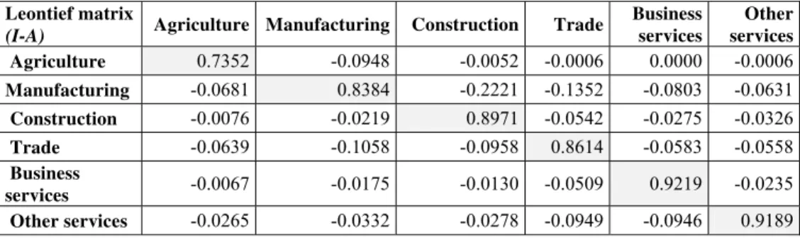
The matrix of input coefficients, A, is called technology matrix. Using the unit matrix, I, with ones on the diagonal, meaning one unit of final demand of each sector, and zeros for all the other elements, the matrix (I - A) is called the Leontief matrix. On the diagonal of the Leontief matrix, there are the proportions of net output for all the other sectors, having positive sign and the meaning of revenues for the considered sector; all the other coefficients are negative, meaning costs for the input requirements.
The Leontief matrix (I - A) of the Romanian economy for 2010, shows the input direct requirements for domestic intermediates in Table 3.
If the input coefficient of Agriculture for its own consumption was of 26.5%, then the net output of Romanian agriculture for all the other sectors represented less than 73.5%, the difference as compared to 100%, as in Table 3, on the diagonal of matrix (I - A).
Leontief matrix
(I-A) Agriculture Manufacturing Construction Trade
Business services
Other services
Agriculture 0.7352 -0.0948 -0.0052 -0.0006 0.0000 -0.0006
Manufacturing -0.0681 0.8384 -0.2221 -0.1352 -0.0803 -0.0631
Construction -0.0076 -0.0219 0.8971 -0.0542 -0.0275 -0.0326
Trade -0.0639 -0.1058 -0.0958 0.8614 -0.0583 -0.0558
Business
services -0.0067 -0.0175 -0.0130 -0.0509 0.9219 -0.0235 Other services -0.0265 -0.0332 -0.0278 -0.0949 -0.0946 0.9189
Table 3.Matrix of direct requirements for domestic intermediates, in 2010
The net outputs for the sectors Business services and Other services were obtained in the greatest proportions, more than 90%, followed closely by the Construction
sector, Trade, Manufacturing – with over 80% and by Agriculture with less over 70%.
The inverse matrix (I - A)-1 is the Leontief inverse and it reflects the direct and indirect requirements of intermediates. The direct input requirements are defined by matrix A. The power matrices of A show the indirect effects from the previous stages of production. The inverse Leontief matrix, (I - A)-1, can be also expressed by the sum of power series of A matrices, as: (I - A)-1= I + A + A2 + A3 +.... + An.
The inverse Leontief matrix for the Romanian economy, in 2010 is presented in Table 4 and shows the direct andindirect input requirements of the economy for one unit of final demand.
The column sums signify the output multipliers of sectors. The output multiplier j is the sum of productions in all sectors of the economy, necessary at all stages of production for producing one unit of final demand j.
For 1 million euro of final demand in Agriculture, the total effect induced in the Romanian economy was 1.763 million euro - the output multiplier of
Agriculture. The direct and indirect requirements represented the internal greatest value of 1.379 million euro, own revenues - induced effect in Agriculture, and 0.384 million euro, the sum of the coefficients from the first column of Table 4 – indirect induced effect in the other economic sectors.
Inverse Leontief matrix
Agriculture Manufacturing Construction Trade Business services
Other services
Agriculture 1.3793 0.1625 0.0524 0.0327 0.0195 0.0165
Manufacturing 0.1463 1.2562 0.3433 0.2404 0.1468 0.1170
Construction 0.0259 0.0466 1.1380 0.0874 0.0487 0.0502
Trade 0.1287 0.1788 0.1795 1.2172 0.1076 0.0954
Business
services 0.0218 0.0374 0.0346 0.0770 1.0976 0.0365
Other services 0.0614 0.0737 0.0704 0.1459 0.1314 1.1081
output
multiplier 1.7633 1.7553 1.8182 1.8007 1.5517 1.4236
Table 4. Direct and indirect requirements for domestic intermediates, in 2010
The output multiplier signifies the cumulative revenues of each sector, meaning one unit of final demand and the direct and indirect requirements for domestic intermediates.
direct effects of agriculture in 2010, 0.0767 - indirect effects of agriculture in previous stage, 0.0243 - indirect effects of two stages ago, 0.0084 - of three stages ago, 0.0031 - of four stages ago, 0.0012 - of five stages ago and close to 0 six stages ago. Starting with the third production stage, the indirect influence was only 0.84%, so less than 1% for the three stages before the third stage.
For the Romanian economy, the Construction and Trade sectors were the most efficient, because they induced the greatest revenues in the economy: at every 1 million of final demand increase, there should be obtained 1.8 million euro in the whole economy. The direct and indirect effects of Construction were the greatest. If the final demand for Construction should increase by 1 million Euros, the cumulative revenues of 1.818 million Euros would be induced in the economy. The
Construction sector had the best output multiplier in Romania, in 2010. The investments in Construction have had the greatest impact, generating the greatest value of cumulative revenues throughout the economy.
3.3. Applications of Leontief input-output model for the Romanian economy
The Leontief input-output model is based on the Leontief equation system. This system has a set of equations for all sectors, where for each sector i, the sum of intermediates xij, and the final demand for commodity of this sector i, gives the output of the same sector, j.
The assumption that all sectors produce with linear Leontief production functions means that the proportions of inputs (intermediates, capital, labor, land) in relation to output are fixed, meaning that the technical input coefficients are the same.
The Leontief equation system considers the final demand as an exogenous variable, y, on the right side of the Eq. 2; the matrix product of technology matrix A
and the vector of outputs x – represents the requirements for intermediates; the net output (without intra-sectoral consumption) x - Ax, is given by the Leontief matrix
(I - A) multiplied by x, which become final demand in Eq. 3. In the Leontief matrix, the outputs will have positive sign, meaning revenues and being on its diagonal and the inputs will have negative sign, meaning costs to other sectors.
Ax + y = x (1)
x – Ax = y (2)
(I - A) x = y (3)
x = (I - A)-1y (4)
In other words, the levels of different industries can be sized for a given level of final demand. So the changes of sectoral final demand, can easily conduct to the required levels of productions for each sector, knowing that the technical coefficients which show the inter-sectoral relationships, remain constant for longer periods. The technology matrix A for the Romanian economy in 2010 is presented in Table 2.
In a deeper analysis the input coefficients for intermediates, could be considered together with those for primary inputs: capital and labor. Macroeconomic models with some sectoral disaggregation could stay at the basis of labor and fiscal policies. The central model of input-output analysis has the central equation system:
Z = B(I - A)-1Y, where:
B = vector of input coefficients for a certain variable: intermediates, labor, capital, energy or emissions;
I = unit matrix;
A = matrix of input coefficients for intermediates;
Y = diagonal matrix for exogenous final demand for goods and services;
Z = matrix with results for direct and indirect influences for the studied variable of intermediates, labor, capital, energy or emissions.
The multipliers are the column sums of coefficients of the matrix product B(I - A)-1
and the values of the analyzed type of input is the matrix product Z.
3.3.1 Primary input content for products of final demand in Romania, in 2010
In order to establish the direct and indirect requirements of Domestic intermediates, the vector B consists of the input coefficients, presented in the last row of Table 2, as the sums of input coefficients of sectors, showing their direct effects on the economy.
The vector product betweenthe vector B and the matrix (I - A)-1 from Table 4, shows the direct and indirect effects in the entire economy of considering the technological matrix, A. These output multipliers of domestic intermediates are presented in Table 5, on the corresponding row.
In order to find the direct and indirect effects of all the inputs of production activities, the vectors of input coefficients B are multiplied by the inverse matrix Leontief (I - A), using the equation z = B(I - A)-1, where z is the vector of output multipliers.
Using input coefficients of ones for Output, the result of output multipliers will be just the values obtained by adding the sectoral output multipliers of the inverse Leontief matrix (I - A)-1, on the last row of Table 4.
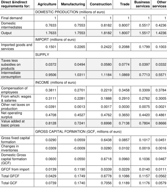
The output multipliers minus the unit of final demand show just the direct and indirect effects on the economy, in 2010, in Table 5.
Direct &indirect
requirements for: Agriculture Manufacturing Construction Trade
Business services
Other services
DOMESTIC PRODUCTION (millions of euro)
Final demand 1 1 1 1 1 1
Domestic
intermediates 0.7633 0.7553 0.8182 0.8007 0.5517 0.4236
Output 1.7633 1.7553 1.8182 1.8007 1.5517 1.4236
IMPORT (millions of euro) Imported goods and
services 0.1501 0.2265 0.2422 0.2088 0.1799 0.1003
SUPPLY Taxes less
subsidies on products
0.0372 0.0494 0.0580 0.0774 0.0397 0.0332
Intermediate
consumption 0.9506 1.0311 1.1184 1.0869 0.7713 0.5571
INCOME (millions of euro) Compensation of
employees 0.3811 0.2701 0.2219 0.3458 0.3309 0.3784
From which: wages
& salaries 0.3111 0.2281 0.1888 0.2910 0.2762 0.3005
Other net taxes on
production -0.0391 0.0013 0.0017 0.0030 0.0075 0.0021
Net operating
surplus 0.4708 0.4527 0.4762 0.3650 0.4420 0.4861
Value added at
basic prices 0.8128 0.7241 0.6998 0.7138 0.7804 0.8666
GROSS CAPITAL FORMATION (GCF, millions of euro)
Gross fixed capital
formation 0.0290 0.0559 0.6438 0.0857 0.1017 0.0451
Changes in
inventories 0.0309 -0.0009 0.0280 0.0102 0.0019 0.0016
Domestic Gross capital formation (GCF)
0.0600 0.0550 0.6718 0.0960 0.1036 0.0467
GFCF from import 0.0139 0.1190 0.0339 0.0229 0.0140 0.0111
Total GFCF 0.0429 0.1749 0.6778 0.1086 0.1157 0.0562
Total GCF 0.0739 0.1740 0.7056 0.1189 0.1176 0.0579
As already concluded, the Construction sector was the best to invest in, because for 1 million euro of final demand the effects were of 1.818 million euro in the entire economy.
The imported goods and services for 1 unit of final demand were the most efficient also in Construction.
The income of Romanian households, received for labor supply, in 2010, is emphasized by the direct and indirect requirements for compensation of employees, from which the wages and salaries, as primary input in order to produce one unit of final demand. Agriculture is the sector where for 1 million euro of final demand, the direct and indirect effects over wages in economy were the greatest.
The sum of output multipliers of Final demand and Domestic intermediates
gives the multiplier of Output from each sector. This relation is also available for the calculated values of these indicators for a certain amount of final demand, from the diagonal matrix of final demand, and found in column 16 of Table 1, for the six sectors.
The sum of output multipliers of Domestic intermediates, Imported goods and services and Taxes less subsidies on products, gives the direct and indirect effects of
Intermediate consumption of each sector, throughout the economy.
The sector Other services brought the lowest direct and indirect effects throughout the economy, with the lowest effects of Imported goods and services and having the lowest effects of Intermediate consumption. But, it can be appreciated that for each final demand of 1,000,000 euro in this sector, there was the greatest
Value added of 866,600 euro, from which a Net operating surplus of 486,100 euro and with only 57,900 euro investment. For this sector the direct effects were the greatest as compared to the others, having the input coefficient of 0.6691. This means that from the direct and indirect effects for Value added of 866,600 euro, the value 669,100 euro represents direct effects.
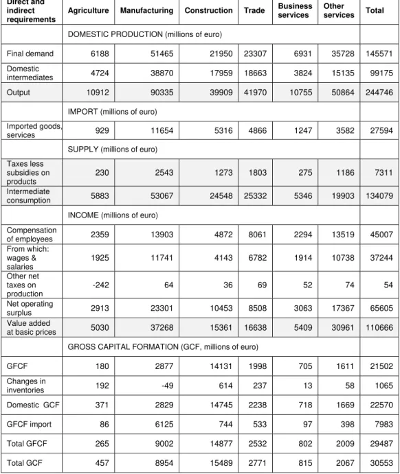
Table 5 contains the multipliers for products which were delivered to final demand in 2010 and Table 6 contains the effects of these multipliers for the sectoral final demand. The content of primary inputs for the production activities, which correspond to the final demand of year 2010, is presented in Table 6.
There are some differences between the theoretical calculated values from Table 6 and the real values from Table 1. The sectoral differences between the theoretical and the effective distribution of indicators are founded on the reasons of practical and theoretical nature. The practical reasons refer to different conditions of productivity and efficiency of each sector.
Direct and indirect requirements
Agriculture Manufacturing Construction Trade Business
services
Other
services Total
DOMESTIC PRODUCTION (millions of euro)
Final demand 6188 51465 21950 23307 6931 35728 145571
Domestic
intermediates 4724 38870 17959 18663 3824 15135 99175
Output 10912 90335 39909 41970 10755 50864 244746
IMPORT (millions of euro)
Imported goods,
services 929 11654 5316 4866 1247 3582 27594
SUPPLY (millions of euro)
Taxes less subsidies on products
230 2543 1273 1803 275 1186 7311
Intermediate
consumption 5883 53067 24548 25332 5346 19903 134079
INCOME (millions of euro)
Compensation
of employees 2359 13903 4872 8061 2294 13519 45007
From which: wages & salaries
1925 11741 4143 6782 1914 10738 37244
Other net taxes on production
-242 64 36 69 52 74 54
Net operating
surplus 2913 23301 10453 8508 3063 17367 65605
Value added
at basic prices 5030 37268 15361 16638 5409 30961 110666
GROSS CAPITAL FORMATION (GCF, millions of euro)
GFCF 180 2877 14131 1998 705 1611 21502
Changes in
inventories 192 -49 614 237 13 58 1065
Domestic GCF 371 2829 14745 2238 718 1669 22570
GFCF import 86 6125 744 533 97 398 7983
Total GFCF 265 9002 14877 2532 802 2009 29487
Total GCF 457 8954 15489 2771 815 2067 30553
The function production describes the dependence of output on the intermediates and on the primary inputs: labor and capital: xj = f(xij, Lj, Cj), where:
xj = output of sector j (products),
xij = flow of goods and services between sector i and j (intermediates),
Lj = required labor of sector j – number of employees is missing, but the wages and salaries describe the income of labor supply,
Cj = required capital of sector j, here is present by investments through domestic and from import Gross Fixed Capital Formation, Changes in inventories, giving Gross Capital Formation,
f = technology – described by matrix A, which contains the input coefficients of intermediates for products and of primary inputs.
The production processes should obtain maximum outputs with the used inputs. The theoretical constructions cannot reproduce exactly the reality, but they can offer a useful tool to understand the interrelations between the sectors of an economy.
3.3.2. Primary input content for final demand, by category of final use, in 2010
The output is formed by the intermediate production and the production for obtaining final demand. The production for the final destinations of consumption is presented in Table 7.
The values of consumption of output production by final uses are obtained using the same model: Z = B(I - A)-1Y = zY, where:
B – input coefficients of the considered primary input,
(I - A)-1 – inverse matrix Leontief of technological matrix A,
Y – the matrix of sectoral output by category of use, is presented in Table 7. The z coefficients of direct and indirect effects of output multipliers are already calculated in Table 4. It remains only to consider them multiplying by matrix Y.
matrix Y Private
consumption
Government
consumption GFCF
Changes in
inventories Exports
Agriculture 3081 562 103 427 2015
Manufacturing 20927 968 1479 -460 28551
Construction 3231 0 17447 758 514
Trade 12069 3342 1017 332 6548
Business services 4358 111 841 4 1618
Other services 18182 15302 485 2 1757
Total by category of
use 61848 20285 21372 1063 41003
The totals obtained for each primary input, in the last column of Table 8, are just the same as those obtained in the analysis of primary input content of production activities of sectors for obtaining the final demand, in the last column of Table 6. The differences between the theoretical structure of output consumption by categories, from Table 8, and the effective distribution of production output for final demand, from Table 7, can be subject of debate for governmental policies.
The private consumption was too high and it should have had to decrease in favor of government consumption, which was underestimated. Also investments have had to increase for GFCF, from 30,725 millions of euro to 38,327 millions of euro and for changes in inventories from 1,063 million of euro to 1,930 millions of euro.
Direct and indirect effects by categories of final
uses
Private consumption
Government consumption GFCF
Changes in
inventories Exports Total
FINAL DEMAND and OUTPUT (millions of euro)
Final demand 61847 20285 21373 1063 41003 145571
Domestic
intermediates – th. 40571 10380 16955 867 30403 99175
Output theoretic 102418 30664 38327 1930 71406 244746
IMPORT (millions of euro) – theoretic values Imported goods and
services 11110 2555 4988 214 8727 27594
SUPPLY (millions of euro) - theoretic values Intermediate
consumption 54727 13774 23160 1144 41274 134079
INCOME (millions of euro) - theoretic values Compensation of
employees 20040 7458 5125 324 12060 45007
From which: wages
& salaries 16522 5998 4337 269 10118 37244
Other net taxes on
production 17 22 37 -15 -7 54
Net operating
surplus 27633 9410 10005 478 18079 65605
Value added at
basic prices 47691 16890 15167 786 30132 110666
Table 8. Primary input content of production by categories of final demand
3.4. Output coefficients of Romanian economy, in 2010
The output coefficients are related to the market shares for commodities and primary inputs of sectors. The calculation of output coefficients consists in dividing each entry of the rows in the input-output table by the corresponding row total. Tables 9 and 10, corresponding to quadrant I and II of Input-Output table, show the output coefficients for domestic intermediates of each sector, defined as: oij = xij/xi, where:
oij = output coefficient domestic goods, services of sector i from sector j (i=1,6; j=1,6)
xij = flow of domestic commodity i to sector j xi = output of sector i.
The proportion of domestic products, 40.5% was distributed for economic sectors: 3.5% for Agriculture, 15% for Manufacturing, 6% for Construction, 9% for Trade, 2% for Business services and 5% for Other services.
Output coefficients
Agricul-ture
Manufac-turing
Construc-tion
Trade Business services
Other services
Total
Agriculture 0.265 0.407 0.008 0.001 0.000 0.002 0.683
Manufacturing 0.016 0.161 0.083 0.075 0.013 0.038 0.386
Construction 0.005 0.058 0.102 0.079 0.012 0.052 0.307
Trade 0.027 0.191 0.065 0.139 0.017 0.060 0.498
Business serv. 0.010 0.108 0.030 0.175 0.078 0.087 0.488
Other services 0.010 0.056 0.018 0.089 0.026 0.082 0.280
Domestic
products 0.035 0.149 0.060 0.090 0.019 0.053 0.405
Agriculture 0.125 0.565 0.021 0.001 0.000 0.002 0.714
Manufacturing 0.024 0.221 0.095 0.102 0.028 0.040 0.510
Construction 0.011 0.143 0.174 0.215 0.029 0.177 0.749
Trade 0.006 0.028 0.016 0.055 0.016 0.041 0.161
Business
services 0.016 0.181 0.053 0.313 0.154 0.172 0.889
Other services 0.018 0.124 0.023 0.189 0.055 0.301 0.711
Imported
products 0.029 0.229 0.086 0.105 0.031 0.052 0.533
Taxes less
subsidies 0.025 0.164 0.074 0.176 0.023 0.074 0.537
Total
intermediates 0.033 0.163 0.065 0.096 0.021 0.053 0.432
The Imported products for the sectoral consumption represented 53.3% of Imported products, being distributed mainly for Manufacturing, in a proportion of 23% and around or less than 10% for the other sectors; the lowest proportion of imports was for the Agriculture sector. So, 43.2% of the Total intermediates were mainly distributed in Manufacturing, and less than 10% in all the other sectors.
In 2010, the domestic output was consumed in proportion of 40.5% by domestic needs of sectors and 59.5% was for Final uses. From the final uses: 33.6% was final consumption expenditure, from witch 25.3% was private consumption and 8.3% was final consumption of government, 9.2% was for investments (Gross Capital Formation – GCF) and 16.8% was the export.
Output coefficients
Total Private cons.
Final cons.
govern-ment
Final cons. expendi-
ture
GCF Exports FOB
Final uses
Total use
Agriculture 0.683 0.158 0.029 0.187 0.027 0.103 0.317 1.000
Manufacturing 0.386 0.250 0.012 0.261 0.012 0.341 0.614 1.000
Construction 0.307 0.102 0.000 0.102 0.574 0.016 0.693 1.000
Trade 0.498 0.260 0.072 0.332 0.029 0.141 0.502 1.000
Business serv. 0.488 0.322 0.008 0.330 0.062 0.120 0.512 1.000
Other services 0.280 0.366 0.308 0.675 0.010 0.035 0.720 1.000
Domestic prod. 0.405 0.253 0.083 0.336 0.092 0.168 0.595 1.000
Agriculture 0.714 0.286 0.000 0.286 0.000 0.000 0.286 1.000
Manufacturing 0.510 0.227 0.000 0.227 0.179 0.083 0.490 1.000
Construction 0.749 0.146 0.000 0.146 0.106 0.000 0.251 1.000
Trade 0.161 0.839 0.000 0.839 0.000 0.000 0.839 1.000
Business serv. 0.889 0.111 0.000 0.111 0.000 0.000 0.111 1.000
Other services 0.711 0.276 0.000 0.276 0.000 0.013 0.289 1.000
Imported prod. 0.533 0.242 0.000 0.242 0.154 0.072 0.467 1.000
Taxes less subs. 0.537 0.361 0.000 0.361 0.102 0.000 0.463 1.000
Final use p.p. 0.432 0.256 0.065 0.321 0.103 0.144 0.568 1.000
Table 10. Output coefficients of total intermediates and final uses, in 2010
A proportion of 46.7% from imported products was for final uses: 24% for private consumption of population and 15% for investments. The output for final use in purchasers’ prices was 43% for the consumption of economic sectors and 56.8% was for final uses: 32.1% for final consumption expenditure, 10.3% for GCF and 14.4% for export.
3.5. Multipliers of production activities in Romanian economy, in 2010
being its demand.The term "backward linkage" characterizes the demand side of the sector, describing the interconnection of the sector with the other sectors from which the inputs are purchased. The increased output of sector j signifies an addition supply for other sectors such as supplementary inputs to be used by other sectors.
The term "forward linkage" characterizes the offer side of the economic activity of a sector and it refers to the relations between the supplying sector and the other sectors to which it sells its output.
For the Romanian economy, in 2010, the backward linkage of each sector is reflected by the column sum of input coefficients, showing the direct requirements for domestic intermediate production, which can be found in the last row of Table 2. The Trade sector is the most demanded for Romanian economy in 2010 with a
backward linkage of 0.4745, as it was already discussed above.
The backward linkages are reflected in a more useful way by the column sums of the inverse Leontief matrix, which show the direct and indirect requirements of Romanian economic sectors, in the last row of Table 4, being the output multipliers. In this case, Construction sector had the highest level of required inputs from other sectors, its backward linkage being 1.8182.
The forward linkages are measured by the row totals of output coefficients, in the last column of Table 11, showing the direct effects of their output. The row sums of elements of inverse matrix (I - A)-1 measure the forward linkage, in the last column of Table 11, showing the direct and indirect effects of their output through the final uses.
Inverse
(I-A)-1 Agriculture Manufacturing Construction Trade
Business services
Other
services total
Agriculture 1.3793 0.6966 0.0844 0.0777 0.0134 0.0421 2.2936
Manufacturing 0.0340 1.2556 0.1288 0.1331 0.0236 0.0697 1.6448
Construction 0.0159 0.1230 1.1369 0.1280 0.0208 0.0792 1.5038
Trade 0.0540 0.3220 0.1215 1.2171 0.0313 0.1028 1.8488
Business serv 0.0314 0.2312 0.0805 0.2643 1.0975 0.1351 1.8399
Other serv. 0.0241 0.1243 0.0446 0.1365 0.0358 1.1090 1.4743
Table 11. Direct and indirect effects of sectoral output throughout final uses
The analysis of inter-sectoral linkages based on Table 12, shows that the
Construction sector is more demand oriented having the greatest backward linkage
of 1.8182 but it has a lower supply of 1.5038. This sector needs more from other sectors than it can offer to the others. This situation is also available for the
Manufacturing sector.
Inter-sectoral Linkages
Effects Agriculture Manufacturing Construction Trade Business services
Other services
Direct 0.4375 0.4346 0.4667 0.4745 0.3387 0.2568
Backward
linkages Direct
and indirect
1.7633 1.7553 1.8182 1.8007 1.5517 1.4236
Direct 0.6827 0.3860 0.3073 0.4981 0.4875 0.2802
Forward
linkages Direct
and indirect
2.2936 1.6448 1.5038 1.8488 1.8399 1.4743
Table 12. Intersectoral linkages in Romanian economy, in 2010
The Other services had the lowest values both for direct and indirect backward linkages and for direct and indirect forward linkages – in the last column of Table 12. Meanwhile, the Agriculture sector is the most supply-oriented, its output being sold into the entire national economy with a multiplier of 2.2936.
4. Conclusions
There are some differences between the uploaded data on Romania, in input-output tables and those updated in the second term of 2015, when the declared Romanian GDP for 2010 amounted to 126,746.4 million euro, instead of 124,328.7 million euro. The Romanian GDP in 2010, transmitted to Eurostat and considered in this paper, was calculated in compliance with ESA95. ESA 2010 has been applicable starting with 2014 (“GDP and main components (output, expenditure and income”,
nama_10_gdp, http://ec.europa.eu/eurostat/data/database).
The paper presents a short introduction into the input-output method.
The Romanian input-output table for 2010 is drawn here only for six sectors, based on the official data transmitted to Eurostat. The calculated structure on six branches is defined as the structure of the European Union’s economic activity characterized by Eurostat by aggregating the national input-output tables of EU Member-states.
Using the input-output table of the Romanian economy in 2010, with indicators in millions euro, current prices, the input and output coefficients were calculated for the economic sectors. Based on the input-output model the output multipliers were used to identify the relative and absolute direct and indirect effects of the economic activity of sectors. The input and output coefficients characterize the inter-sectoral backward and forward linkages and their direct and indirect effects.
The technical matrix of input coefficients allowed the analysis of the inputs of production activities and the primary input content of products for final demand in Romania, in 2010, and by category of final uses.
In 2010, the agricultural profile of the Romanian economy was identified, by its main role, having the greatest multiplier of forward linkages in the entire economy. The effects of the Agriculture sector for the future development of Romanian economy should be considered for European financing programs and for the investments policies in this sector.
Every change of taxes, of wages, of prices, of imports, of exports, of investments and others, can be tested with the input-output analysis to see in advance, what effects they can induce in the complex body of the national economy.
5. Acknowledgements
The authors would like to acknowledge that this paper has been written with the support of material documentation during the Erasmus+ teaching mobility at University of Piraeus, Greece, June 2016.
6. References
Kucera, D. and Roncolato, L., 2013. Structure Matters: Sectoral Drivers of Growth and the Labour Productivity–Employment Relationship. In: Islam I., Kucera D. (Eds.) Beyond Macroeconomic Stability. Structural Transformation and Inclusive Development, Advances in Labour Studies. Palgrave Macmillan and the International Labour Office, UK, chapter 4, p. 133-197
Lipinski, Cz., 1985. Changes of Output Capacity Utilization Caused by Structural Changes of Material Inputs. In: Input-Output Modeling Proceedings of the Sixth IIASA (International Institute for Applied Systems Analysis) Task Force Meeting on Input-Output Modeling, Warsaw, Poland, December 16-18, 1985, Springer-Verlag Berlin GmbH, Ed. Tchijov I., Tomaszewicz L., p. 99-106. Available at: http://gen.lib.rus.ec/book/index.php?md5= 435A16D02DDCDDF138B2BB61DD222EF0&tlm=2016-04-03%2005:51:08 Miller, R. E. and Blair, P. D., 2009. Input-output analysis: Foundations and
http://www.usp.br/nereus/wp-content/uploads/MB-2009-05-Ch-2-Found-I-O-Anal.pdf
Miyazawa, K., 1925. Input-Output Analysis and the Structure of Income Distribution”, Lecture Notes in Economics and Mathematical Systems. In: Beckmann M., Kunzi H. P. (Eds.) Mathematical Economics 116, Springer-Verlag Berlin, 1976.
Nübler, I., and Ernst, C., 2013. “Creating Productive Capacities, Employment and Capabilities for Development: The Case of Infrastructure Investment”. In: Islam I., Kucera D. (Eds.), Beyond Macroeconomic Stability. Structural Transformation and Inclusive Development, Advances in Labour Studies,
Palgrave Macmillan and the International Labour Office, UK, chapter 5, pp. 198-227.
Sand, P., 1985. The Use of Impact Tables in Policy Applications of Input-Output Models. In: Tchijov I., Tomaszewicz L (eds.), Input-Output Modeling Proceedings of the Sixth IIASA (International Institute for Applied Systems Analysis) Task Force Meeting on Input-Output Modeling, Warsaw, Poland, December 16-18, 1985, Springer-Verlag Berlin GmbH, Ed.., p. 27-44, http://gen.lib.rus.ec/book/index.php?md5=435A16D02DDCDDF138B2BB61 DD222EF0&tlm=2016-04-03%2005:51:08
Thijs ten Raa, 2006. The Economics of Input-Output Analysis. Cambridge: Cambridge University Press, www.cambridge.org/9780521841795
Eurostat. GDP and main components - Current prices [nama_gdp_c] Last update: 13-04-2015, [online] Available at: http://appsso.eurostat.ec.europa. eu/nui/submitViewTableAction.do [Accessed August 2015]
Eurostat. “GDP and main components (output, expenditure and income)” (nama_10_gdp), [online] Available at: http://ec.europa.eu/ eurostat/data/database [Accessed August 2015]
Eurostat. GDP and main components (nama_10_gdp), [online] Available at: http://ec.europa.eu/eurostat/data/database [Accessed August 2015]
Eurostat. Romania_suiot_131108_eur_cur.xls. [online] Available at: http://appsso.eurostat.ec.europa.eu/nui/submitViewTableAction.do,
updated in 8 November 2013. [Accessed August 2015]
Eurostat, 2008. Eurostat Manual of Supply, Use and Input-Output Tables, p. 480, 481-485, 497. [online] Available at: http://ec.europa.eu/eurostat [Accessed August 2015]
Eurostat. [online] Available at: http://data.worldbank.org/ indicator/ NY.GDP.MKTP.KD.ZG/countries [Accessed August 2015]
Eurostat. [online] Available at: http://ec.europa.eu/eurostat/web/esa-supply-use-input-tables/methodology/supply-use-tables [Accessed August 2015]
Eurostat. [online] Available at: http://ec.europa.eu/eurostat/web/esa-supply-use-input-tables/methodology/supply-use-tables [Accessed August 2015]
Eurostat. [online] Available at: “Technical Documentation eeSUIOT project: Creating consolidated and aggregated EU27 Supply, Use and Input- Output Tables, adding environmental extensions (air emissions), and conducting Leontief-type modelling to approximate carbon and other 'footprints' of EU27 consumption for 2000 to 2006”, Eurostat & Joint Research Centre, p 47-55)
[accessed in August 2015]