Nonequilibrium phase transitions in interacting particle systems.

(1)

Nonequilibrium Phase Transitions in

Interacting Particle Systems

(Transi¸c˜oes de Fase de N˜ao-equil´ıbrio em Sistemas de Part´ıculas Interagentes)

Adriana Gomes Moreira

Tese apresentada à Universidade Federal de Minas Gerais como requisito parcial para a obten¸cão do grau de Doutor em Ciências (F´ısica)

Orientada pelo Professor Ronald Dickman

Co-orientada pelo Professor Jafferson Kamphorst Leal da Silva

(2)

Acknowledgements

I would like to thank

Professor Ronald Dickman, for being such a dedicated advisor, teaching me so much and encouraging me through the hard moments, and mostly, for being my friend.

Professor Jafferson K. Leal da Silva, for nicely guiding my first steps into science.

My beloved Carlos, for supporting me throughout this journey, comforting me with nice words and a beautiful smile.

My beloved family, that with their unconditional love made of me a very happy human being.

My adorable friends, T´eia, Let´ıcia, Heliana, Fabienne and Suely for the support, nice conversations and useful advices.

All my friends for the affection that gave me strength to go on.

Professor Luiz Paulo Vaz, for all the help and patience in computer matters.

Iwan Jensen, for helping me so much (even not being aware of that).

Professors Tânia Tomé Martins de Castro (USP), Wagner Figueiredo (UFSC), Antônio Sérgio Teixeira Pires (UFMG) and João Florêncio Júnior (UFMG) for kindly accepting to take part in the committee, and for helpful suggestions.

(3)

Index

Abstract 1

Resumo 2

1 Introduction 3

2 Introduction to Nonequilibrium Phase Transitions 5

2.1 Introduction . . . 5

2.2 Basic Concepts . . . 5

2.3 Contact Process and Related Models . . . 6

2.4 Scaling Behavior . . . 9

2.4.1 Steady-state Behavior . . . 9

2.4.2 Time-dependent Behavior . . . 11

2.5 Analytical Methods . . . 12

2.5.1 Mean-field Theory . . . 13

2.5.2 Mean-field Renormalization Group . . . 14

2.5.3 Series Expansions . . . 16

2.6 Universality . . . 17

2.7 Disordered Systems . . . 19

3 Diluted Contact Process - Mean-field Theory 22 3.1 Introduction . . . 22

3.2 The Model . . . 23

3.3 Mean–field Cluster Expansions . . . 24

3.3.1 (n, m)-Cluster Approximation . . . 24

3.3.2 Site-approximation . . . 26

3.3.3 Pair-approximation . . . 26

(4)

4 Diluted Contact Process - Simulations 31

4.1 Introduction . . . 31

4.2 The Model . . . 31

4.3 Steady-state Behavior . . . 32

4.3.1 Simulation Results . . . 33

4.4 Time-dependent Behavior . . . 34

4.4.1 Scaling Ansatz . . . 34

4.4.2 Simulation Results . . . 36

4.5 Power-law Relaxation . . . 44

4.6 Summary . . . 47

5 Series Expansions in Pair-contact Process 49 5.1 Introduction . . . 49

5.2 The model . . . 50

5.3 Operator Formalism . . . 51

5.4 Time-dependent Perturbation Theory . . . 55

5.5 A few terms for the one-dimensional PCP . . . 58

5.6 Computer Algorithm . . . 60

5.7 Results and Analysis . . . 61

6 Conclusions and Outlook 67

Appendix 69

(5)

Abstract

We study the two-dimensional contact process (CP) with quenched disorder in the form of random dilution of a fractionx. A qualitative picture of the phase diagram is obtained through mean-field theory (MFT). Monte Carlo simulations show that the relative shift in the critical point, [λc(x)−λc(0)]/λc(0) is in reasonable agreement with

MFT, for small values ofx. As expected on the basis of the Harris criterion, the critical exponents governing the order parameter and the survival probability take values different from those of the pure model. We also study the critical spreading dynamics of the diluted model. In the pure model, spreading from a single particle at the critical pointλc(0) is characterized by the critical exponents of directed percolation: in 2 + 1

dimensions,δ = 0.46, η= 0.214, and z = 1.13. Disorder causes a dramatic change in the critical behavior of the contact process.

(6)

Resumo

Estudamos o processo de contato dilu´ıdo (DCP) bidimensional. Desordem é intro-duzida na forma de dilui¸cão, com uma fra¸cão x de s´ıtios sendo removida aleatori-amente da rede. Uma descri¸cão qualitativa do diagrama de fases é obtida através da teoria de campo médio na aproxima¸cão de blocos. Simula¸cões de Monte Carlo mostram que o deslocamento relativo do ponto cr´ıtico, [λc(x)−λc(0)]/λc(0), para x

pequeno, está de acordo com os resultados obtidos por campo médio. Os expoentes cr´ıticos relacionados com o parâmetro de ordem e a probabilidade de sobrevivência do modelo dilu´ıdo são diferentes dos expoentes do modelo puro, como era esperado pelo critério de Harris. Usando simula¸cões dependentes do tempo estudamos a evolu¸cão do modelo a partir de uma única semente. No modelo puro, o comportamento cr´ıtico é caracterizado por leis de potência descritas pelos expoentes cr´ıticos de percola¸cão dirigida: em 2+1 dimensões,δ = 0.46,η = 0.214, ez= 1.13. A presen¸ca de desordem causa uma mudan¸ca drástica no comportamento cr´ıtico do modelo.

(7)

Chapter 1 Introduction

Statistical mechanics has been used to describe systems in equilibrium quite success-fully. In these systems, statistical fluctuations are due either to thermal agitation or to impurities. In the past few decades, general theories of phase transitions and also of critical phenomena have been developed, unifying understanding of the liquid-vapor transition, magnetic transitions, liquid crystals, and other systems. Understanding of critical phenomena innonequilibriumsteady states, is still developing, however. Since the steady-state probability distribution in these systems is not known a priori, anal-ysis of nonequilibrium systems must be based upon their dynamics. Some of these systems have been found to exhibit a nonequilibrium phase transition, which is marked by a boundary between an active steady state and an absorbing state. Attempts at a better understanding of nonequilibrium phase transitions have led statistical physi-cists to study numerous models, such as reaction-diffusion systems, driven diffusive lattice gases and Ising models with competing dynamics.

In this work we are mainly interested in the issue of universality of critical be-havior, which has been a prime theoretical motivation for studying critical phenomena. In particular we investigate the effects of quenched disorder on the critical behavior of the contact process, an interacting particle system exhibiting a continuous phase tran-sition to a unique absorbing state. A typical interacting particle system, possessing an absorbing state, consists of many particles evolving according to a Markov pro-cess governed by irreversible transition rules. We also study the pair-contact propro-cess, a model with multiple absorbing configurations, whose critical spreading dynamics presents nonuniversal behavior.

(8)

(9)

Chapter 2 Introduction to Nonequilibrium

Phase Transitions

2.1 Introduction

This chapter has the aim of introducing the reader to a particular class of nonequilib-rium models – interacting particle systems exhibiting a continuous phase transition to an absorbing state.

We consider the following topics. In section (2.2) we review some basic con-cepts in critical phenomena. In section (2.3) we discuss the contact process (CP) and related models. In section (2.4) we review scaling behavior in critical phenomena. A brief introduction of the most useful methods applied to nonequilibrium models is given in section (2.5). We discuss universality in section (2.6), and in section (2.7) we give an overview on basic concepts of disordered systems.

2.2 Basic Concepts

(10)

individuals recover at unit rate, and are then susceptible to reinfection. Since an individual must have at least one sick neighbor to become infected, the state in which all the individuals are healthy isabsorbing. An absorbing state is a configuration from which the system cannot escape.

The persistence of the epidemic is controlled by the infection parameter. Ifλis too small, extinction of the infection at long times is certain; on the other hand, large values of λ assure that the infection will spread indefinitely. The boundary between persistence and extinction is marked by acritical point, which is denoted by λc. The

critical parameterλcseparates the two possible steady statesthe system can reach at

asymptotic times, namely a disease-free or absorbing state and a surviving epidemic or active state. It turns out thatλc marks a continuous phase transition between an

absorbing state and an active state. In a continuous phase transition the stationary density of infected individuals (ρ) rises continuously from zero as the infection pa-rameter is increased. A quantity like ρis referred to as an order parameter. Near the critical point the order parameter goes to zero following a power law characterized by acritical exponent: ρ∼(λ−λc)β whereβ is the critical exponent associated with the

order parameter. The independence of the critical exponents on most system details is known as universality. Models with the same set of critical exponents form a uni-versality class. In general a uniuni-versality class is determined by global features such as dimensionality, dimension of the order parameter and range of the interactions.

Models possessing a continuous transition into a unique absorbing state gener-ally belong to the same universality class as the directed percolation (DP), according to the DP conjecture [3, 4, 5, 6]. The presence of conservation laws can influence the critical behavior of a model. Also models with multiple absorbing configurations have presented a non-DP time-dependent behavior [39, 40, 41].

2.3 Contact Process and Related Models

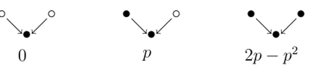
In this section we present a few models that exemplify the main properties of nonequi-librium phase transitions. We start by defining the contact process as a model for creation and annihilation of particles on a lattice, followed by directed percolation and the Ziff-Gulari-Barshad (ZGB) surface-reaction model.

(11)

◦ ◦ ց ւ

0 •

• ◦

ց ւ p

•

• •

ց ւ 2p−p2

•

Figure 2.1: Diagram showing the rules for the directed percolation with bond probability

pon the square lattice.

at unit rate, independent of the surrounding configuration. The order parameter is the stationary particle density; it vanishes in the vacuum state, which is absorbing. As λ is increased beyond λc, the model presents a continuous phase transition from

the vacuum to an active steady state.

Directed percolation (DP) [7] can be defined as the ordinary bond percolation problem, in which bonds are randomly distributed on a lattice with concentrationp, with the introduction of a preferential direction to the problem. Fig. (2.1) shows the transition rules for directed bond percolation. The top row of Fig. (2.2) represents the initial state, which is connected by diagonal bonds to the row below. Each of these oriented bonds is present only with probability p independent of the other bonds. A site in this lattice is connected to the origin if and only if it is connected to a site in the previous layer that is connected to the origin. There is a critical concentrationpc,

below which the probability of an infinite “percolating” cluster is zero. Near pc the

system features the characteristic lengthsξ⊥ and ξk, perpendicular to and parallel to

the main direction, respectively, that diverge like

ξ⊥∼(pc−p)−ν⊥ (2.1)

ξk ∼(pc−p)−νk (2.2)

(12)

◦ ◦ ◦ ◦ ◦ ◦ ◦ ◦ ◦ ◦ ◦ ◦ ◦ ◦ ◦ ◦ ◦ ◦ ◦ ◦ ◦ ◦ ◦ ◦ ◦ ◦ ◦ ◦ ◦ ◦ ◦ ◦ ◦ ◦ ◦ ◦ ◦ ◦ ◦ ◦ ◦ ◦ ◦ ◦ ◦ ◦ ◦ ◦ ◦ ◦ ◦ ◦ ◦ ◦ ◦ ◦ ◦ ◦ ◦ ◦ ◦ ◦ ◦ ◦ ◦ ◦ ◦ ◦ ◦ ◦ ◦ ◦ ◦ ◦ ◦ ◦ ◦ ◦ ◦ ◦ ◦ ◦ ◦ ◦ ◦ ◦ ◦ ◦ ◦ ◦ ◦ ◦ ◦ ◦ ◦ ◦ ◦ ◦ ◦ ◦ ◦ ◦ ◦ ◦ ◦ ◦ ◦ ◦ ◦ ◦ ◦ ◦ ◦ ◦ ◦ ◦ ◦ ◦ ◦ ◦ ◦ ◦ ◦ ◦ ◦ ◦ ◦ ◦ ◦ ◦ ◦ ◦ ◦ ◦ ◦ ◦ ◦ ◦ ◦ ◦ ◦ ◦ ◦ ◦ ◦ ◦ ◦ ◦ ◦ ◦ ◦ ◦ ◦ ◦ ◦ ◦ ◦ ◦ ◦ ◦ ◦ ◦ ◦ ◦ ◦ ◦ ◦ ◦ ◦ ◦ ◦ ◦ ◦

ց ց ց ց ց ց ց ց ց ց ց

ւ ւ ւ ւ ւ ւ ւ ւ ւ ւ ւ

ց ց ց ց ց ց ց ց ց ց ց

t ↓

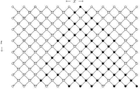
← x → ◦ ◦ ◦ ◦ ◦ ◦ ◦ ◦ ◦ ◦ ◦ • • • • • • • • • • • • • • • • • • • • • • • • • • • • • • • • • • • • • • • • • • • • • • • • • • • • • • • • • • • • • • • • • • •

Figure 2.2: Typical time evolution from a single particle in dynamical directed percolation, particles are represented by a •, lattice sites by a ◦, and the directed bonds by arrows. The cluster is typical of those observed at large values of the spreading probabilityp.

site itself were occupied in layert−1 (this avoids spontaneous creation). A site can be vacant in layerteven if it is occupied in layert−1 (annihilation). Directed percolation is the simplest way of implementing this simultaneous updating. Thus “survival” of a trial in the CP corresponds to “percolation” in DP. Although one model cannot be mapped onto the other, the CP and DP are equivalent as far as critical behavior is concerned.

A wide variety of catalysis models have been considered in the study of nonequi-librium phase transitions. Perhaps the best known is the Ziff-Gulari-Barshad (ZGB) model for the oxidation of carbon monoxide (CO) on a catalytic surface [12]. Such reactions are of great technological importance. The model is defined on a square lat-tice, which represents the catalytic surface. The reaction proceeds via the Langmuir-Hinshelwood mechanism: both species must be chemisorbed. Adsorption of CO molecules occurs at rate y on a vacant site; adsorption of O2 requires a

nearest-neighbor pair of empty sites. Adsorbed O and CO react when they are sitting at nearest-neighbor sites, followed by the immediate desorption of the product, CO2

(13)

is absorbing. Depending on y, the system can exist in one of three phases: poisoned by O, poisoned by CO, or reactive. The model presents a first order phase transi-tion from the CO-poisoned to the active state, and a continuous transition from the oxygen-covered state to the active state. This latter belongs in the universality class of directed percolation [3, 14, 15].

2.4 Scaling Behavior

The idea of scaling, which is strongly associated with continuous phase transitions, was first introduced on a phenomenological basis by Widom [16]. He conjectured that the equation of state is a homogeneous function of the relevant thermodynamic variables in the vicinity of the critical point. Near the critical point, the system is subject to strong fluctuations correlated over very large times and distances, being characterized by a divergence of the correlation length at the critical point. Based on this fact, Kadanoff [17] gave an intuitive picture for scaling. The scaling hypothesis states that the divergence of the correlation length is responsible for the singular dependence of physical quantities on the distance from the critical point. Scaling gained a firmer basis with the advent of the renormalization group devised by Wilson [18].

2.4.1 Steady-state Behavior

As we have already seen, a nonequilibrium phase transition occurs in the stationary regime (between the stationary absorbing state and an active stationary state). In the following we try to give an idea of the main aspects of steady-state critical behavior.

Critical Behavior

Near the critical point, thermodynamic response functions are dominated by a singular contribution, associated with a diverging correlation length. The singu-lar contribution depends (in the simplest cases) on a single variable, the correlation length, and generalized homogeneity reflects how the correlation length depends on the relevant thermodynamic variables. The latter, in equilibrium, are reduced tem-perature and field, or reduced chemical potential in a fluid system.

(14)

a functionF(x) is homogeneous if it satisfies,

F(λx) =g(λ)F(x) (2.3)

for all values of the parameter λ. The function g(λ) must always be power-like, g(λ) =λp_{. Analogously, for a homogeneous function of two variables we have}

F(λx, λy) = λpF(x, y). (2.4)

Generalized homogeneity involves different scaling dependencies upon two (or more) arguments, so:

F(µux, µvy) = µpF(x, y). (2.5) By setting λ=µp _{we get}

F(λupx, λ v

py) =λF(x, y) (2.6)

F(λax, λby) =λF(x, y) (2.7)

wherea=u/pandb=v/p. Thus a generalized homogeneous function is characterized by two (or more) powers, herea and b.

As critical behavior of thermodynamic variables is described by generalized homogeneous functions we expect that such quantities as the order parameter, sus-ceptibility, etc., follow power-laws near the critical point [16]. Hence the stationary density near the critical point, (λ > λc), grows as

ρ_• ∝ |λ−λc|β (2.8)

where β is the order parameter critical exponent. As in equilibrium critical phe-nomena, nonequilibrium systems, undergoing a continuous phase transition, feature a characteristic length scale, the correlation length (ξ), near the critical point. The correlation length diverges at criticality as

ξ ∝ |λ−λc|−ν⊥ (2.9)

whereν⊥ is the correlation-length exponent. The relaxation time,τ, the time it takes

for a system to reach the steady state, also diverges at the critical point,

τ ∝ |λ−λc|−νk, (2.10)

(15)

Finite-size Scaling

In a finite system, the correlation length cannot become infinite, since it is limited by the linear extent of the system,L. The singularities that characterize phase transitions and critical points only emerge in the limitL→ ∞; in finite systems they are rounded over a region roughly delimited by ξ ≥ L, where ξ is the correlation length in the infinite-size limit. Next we show how to use this size-dependence to locate the critical point and estimate exponents.

As we are working in a finite volume, we expect that finite-size effects become relevant near the critical point, as the infinite-size correlation length ξ ≈ L. Thus, according to finite-size scaling hypothesis [20, 21], various quantities depend on the system size through the ratioL/ξ, or equivalently through the variable ∆L1/ν⊥_{, where}

∆≡ |λ−λc|. For example, expressing the order parameter as a function of ∆ and L,

we have

ρ_•(∆, L)∝L−β/ν⊥_f(∆L1/ν⊥_). _(2.11)

We must assume that f(x)∝xβ _for _x_{→ ∞}_{in order to recover Eq. (2.8) in the limit}

L→ ∞. At the critical point, ∆ = 0, we obtain

ρ_•(0, L)∝L−β/ν⊥_. _(2.12)

Log-log plots of the stationary density versus the system size can be very useful in locating the critical point.

2.4.2 Time-dependent Behavior

We cannot talk about scaling behavior without mentioning the time-dependent anal-ysis introduced by Grassberger and de la Torre [22]. The basic idea is to study the spread of a population starting from a configuration close to the absorbing state, in general a single seed at the origin. Of prime interest are P(t), the probability that the system has not entered the absorbing state at time t, n(t), the mean number of particles (averaged over all trials, including those that do not survive until time t), and R2_{(t), the mean-square distance of particles from the origin. In the subcritical}

region, λ < λc, P(t) and n(t) decay exponentially. In this regime, as annihilation is

the dominant event the population cannot spread very far, thus we expectR2_(t)_∝_t.

(16)

a single particle at the origin at t = 0, decays exponentially at long times and large distances:

ρ(r, t)≃exp(−r/ξ) exp(−t/τ), (2.13) whereξandτ are the characteristic spatial extent and the characteristic lifetime, both diverging asλ→λc. Thus a cluster emanating from a single seed has a characteristic

lifetimeτ and spatial extentξ. In the supercritical regime,(λ > λc), there is a nonzero

probability that the process continues to spread from this seed as t→ ∞; the active region expands at a constant rate, so that n(t) ∝ td _and _R2_(t) _∝ _t2_{. The process}

dies out with probability one at the critical point, but the mean lifetime diverges. In the absence of a characteristic time scale, the asymptotic evolution of these quantities follows power-laws,

P(t)∝ t−δ _(2.14)

n(t)∝ tη _(2.15)

R2(t)∝ tz _(2.16)

where δ, η and z are critical exponents. Thus log-log plots of P(t), n(t) and R2_(t)

approach straight lines at the critical point, and show a positive or negative curvature in the supercritical or subcritical regimes, respectively. The exponents δ, η and z are provided by the asymptotic slopes of the critical curves. In general we have to expect finite-time corrections to scaling of the type

P(t)∝t−δ(1 +at−θ+bt−δ′ +· · ·). (2.17) Similar expressions hold for n(t) and R2_{(t). This implies for the local slope} _{δ(t) the}

behavior

δ(t) =δ+at−θ+bt−δ′ +· · ·, (2.18) and analogous expressions forη(t) andz(t).

2.5 Analytical Methods

(17)

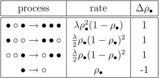
process rate ∆ρ•

• ◦ • → • • • λρ2

•(1−ρ•) 1

• ◦ ◦ → • • ◦ λ

2ρ•(1−ρ•)

2 ₁

◦ ◦ • → ◦ • • λ

2ρ•(1−ρ•)

2 ₁

• → ◦ ρ• -1

Table 2.1: Rates of change for the one-dimensional contact process in site-approximation level. • represents a particle and ◦ a vacancy.

one-dimensional contact process. Then we present an example of the mean-field renor-malization group which, in general, leads to better estimates of critical parameters than the ones obtained by mean-field theories. A brief summary of the basic idea of series expansions follows.

2.5.1 Mean-field Theory

We consider the CP as defined in section (2.3) with d = 1. Let σi = 1 represent the

state of sitei when occupied by a particle, and σi = 0 when vacant. The probability

that sitei is occupied at time t is represented by P(σi = 1;t) ≡ρ•. In Table 2.1 are

summarized the rates of change for each process of the one-dimensional CP. In the first process creation occurs at the central site at rateλ; by treating each site independently and assuming spatial homogeneity one can write the probability for finding the cluster in this configuration asρ2

•(1−ρ•). Each contribution to the evolution equation is given

by the product of the rate of change and the change in the number of particles, ∆ρ•.

Thus, considering the four possible events showed in Table 2.1, the equation of motion forρ• is given by

dρ•

dt =ρ•(λ−1)−λρ

2

•. (2.19)

Forλ≤ 1 the only stationary solution is the vacuum,ρ• = 0. For λ >1 we also find

an active stationary solution, namely ρ• = 1−λ−1. We can see that for λ > λc = 1

the active state is stable and the vacuum unstable. λcmarks a critical point, at which

the stationary density changes continuously but in a singular manner. Thus ρ• is the

order parameter for this transition, assuming a nonzero value only forλ > λc. Near

the critical point the order parameter generally follows a power law,

(18)

where ∆≡λ−λc. Hence, in the mean-field approximation of the CP we find β = 1,

asρ• = ∆ +O(∆2) for ∆>0. This simple mean-field analysis predicts a qualitatively

correct phase diagram, while it provides very poor values for the critical point and exponents. This is a direct consequence of neglecting any correlations among the sites; in fact they are highly correlated. It is worth remarking that the mean-field exponents are incorrect for spatial dimensions d < dc = 4, where dc is the upper

critical dimension, above which the critical exponents are field like. In mean-field theory one assumes that all neighbors of a given site behave in the same way. Spatial homogeneity is also realized in high dimensionality. Therefore it is reasonable to expect that mean-field theory is exact in the limit of larged. In fact, most systems have a particular dimensionality, known as its critical dimensionality, above which mean-field theory gives the right description of critical properties.

2.5.2 Mean-field Renormalization Group

The mean-field renormalization group (MFRG) has been successfully employed in nonequilibrium systems [24, 25, 26]. The method can be seen as a combination of the usual mean-field and renormalization group ideas.

As an example of a MFRG analysis we apply it to the one-dimensional contact process. By considering a two-site cluster we study the evolution of the probability of finding sites i and j in states σi and σj at time t, P(σi, σj;t). σ can take the values

{0,1} indicating a vacant and an occupied site, respectively. In order to simplify the notation we denote P(1,1;t)≡ ρ••, P(0,0;t) ≡ρ◦◦, and P(0,1;t) +P(1,0;t) ≡ ρ•◦.

Thus, for a two-site cluster we get: dρ◦◦

dt = −λxρ◦◦+ρ•◦ dρ•◦

dt = − 1

2ρ•◦λ(1 +x)−ρ•◦+ 2ρ••+λxρ◦◦ (2.21) dρ••

dt = −2ρ••+ 1

2λρ•◦(1 +x)

where x is the probability of any site outside the cluster being occupied. As we are studying a continuous phase transition we may let the fieldxbecome arbitrarily small in the vicinity of the critical point. Thus the order parameterρ(2)

• (λ, x) (for the 2-site

cluster) can be linearized in x. In the steady state one obtains

ρ(2)_• ≡ρ••+

1

2ρ•◦=x( λ 2 +

λ2

4 ) +O(x

(19)

Applying the same reasoning to a one-site cluster, the evolution equation forP(1;t)≡ ρ• is simply

dρ•

dt =−ρ•+λ

′₍₁₋_ρ

•)x′, (2.23)

where x′ _{is the probability that any other site is occupied, and} _λ′ _{is the creation}

parameter for the one-site cluster. Notice that if we letρ• =x′ we recover the

mean-field site approximation of eq. (2.19). In the steady state, and expanding in x′_{, we}

find ρ• ≈λ′x′+O(x′2).

The main assumption of MFRG is that the two approximate order parameters rescale in the same manner as the two fields. Thus, on the basis of a Wilson renor-malization group strategy [18], a mapping (λ, x)→(λ′_{, x}′_{) is obtained by requiring}

ρN_•′(λ′, x′) =Ld−yρN_• (λ, x) (2.24)

x′ =Ld−yx (2.25)

to hold to leading orders in x. L is the length-rescaling factor associated with the two clusters L = (N/N′₎1/d_{. The exponent (d}₋_{y) is the scaling dimension of the}

order parameter. An estimate for the critical point, λc, may be found by expanding

eq. (2.24) for smallx, leading to a relationλ′ ₌_f_{(λ), from which}_λ

cmay be determined

by locating the fixed point(s) of this transformation. Thus, assuming that ρ•(λ′, x′)

and ρ(2)

• (λ, x) scale like x′ and x, respectively, we find the recursion relation

λ′ = λ 2 +

λ2

4 , (2.26)

which has the fixed pointλc= 2. This represents a substantial improvement over the

one-site value. (Naturally, better results are achieved using even larger clusters.) For the one-dimensional CP, series expansions [27] and simulations [22] yieldλc≃3.2978.

The method also provides estimates for the critical exponents. As an example we compute the correlation length exponent defined through the relation,ξ∼(λ−λc)−ν⊥.

After a rescaling the new correlation length will be

ξ′ ∼L−1ξ, (2.27)

which in terms ofλ and λ′ _becomes

(20)

If the transformation λ′ ₌ _f_{(λ) is regular (Wilson’s fundamental assumption), we}

may linearize it around the fixed point:

(λ′−λc) = (λ−λc)[

∂λ′

∂λ]λ=λc (2.29)

which together with eq. (2.28) gives

[∂λ

′

∂λ]λ=λc ∼L

1/ν⊥_. _(2.30)

In our example L= (N/N′_{) = 2, and from the recursion relation we find that}

[∂λ′_{/∂λ] = 3/2 at} _λ

c. Thus

ν⊥ =

ln 2

ln 3/2 = 1.71, (2.31)

that should be compared to ν⊥ = 1.100(5) obtained from transfer-matrix methods

[28].

2.5.3 Series Expansions

Series expansions have been of great importance in the study of nonequilibrium sys-tems [14, 27, 29, 30], and are probably the most precise method available. Unfor-tunately, its application to the CP and related models is limited to low dimensional systems.

One is typically interested in finding the critical parameters of some function F(z) that exhibits a power-law behavior in the vicinity of a critical point zc, i.e.,

F(z)≈A(zc−z)−α. (2.32)

IfF is analytic in the neighborhood of the origin it is possible to represent it through a Taylor series,F(z) =P∞_j₌₀ajzj. One begins a series analysis by determining as many

terms as possible in this expansion. Once one has the series one needs a method for extracting the critical parameters. The method of Pad´e approximants [31, 32, 33, 34] provides a powerful general technique for approximating a function F(z), having simple poles atz1,· · ·, zn. One assumes that the series for F(z) is the expansion of a

ratio

F(z)∼ PN(z) QM(z)

≡ p0+p1z+· · ·+pNz

N

q0+q1z+· · ·+qMzM

(2.33)

(21)

series coefficients of the expansion of F(z). The usefulness of these approximants comes from the fact that a function like F(z) will have a logarithmic derivative of the form dlnF(z)/dz and a simple pole at zc, which is very well represented by Pad´e

approximants. If the series is well behaved the critical point is associated with the first singularity on the positive real axis. Thuszc is given by locating the pole of the

Pad´e approximant and the critical exponent is the corresponding residue.

2.6 Universality

Universality of critical behavior has been a central topic in the study of continuous phase transitions. The fact that many different models can belong to the same univer-sality class shows the irrelevance of the microscopic characteristics and, at the same time, a strong dependence on general properties such as system dimension, dimension of the order parameter, range of the interactions, conservation laws, etc. One of the most important achievements in nonequilibrium phase transitions is that a wide va-riety of models exhibiting a continuous transition into a unique absorbing state have been shown to belong to the same universality class as directed percolation [13, 3, 4, 5]. So far we have seen that changes in the dynamics, like inclusion of diffusion, multi-particle processes, multiple components, sequential versus parallel updating, do not seem to alter the critical behavior of the models. Several examples confirm that the DP universality class is very robust. The two-component ZGB model exhibits a second-order phase transition of the DP kind [15]. Various cellular automata for surface reactions (simultaneous-update versions of the ZGB model) have been studied [35, 36] and found to have a critical behavior consistent with directed percolation. A basis for universality appears in field theory, providing one can show that the contin-uum descriptions for various models differ only by irrelevant terms. In field theory the microscopic picture of particles on a lattice is replaced by a set of densities which evolve via stochastic partial differential equations (Langevin equations). Janssen [4] proposed a continuum description of the CP and allied models:

∂ρ(~x, t)

∂t =aρ(~x, t)−bρ(~x, t)

2₋_{cρ(~x, t)}3₊_{. . .}₊_D∇2_{ρ(~x, t) +}_{η(~x, t),} _(2.34)

where ρ(~x, t)≥ 0 is the particle density; the ellipsis represents terms of higher order in ρ(~x, t). η(~x, t) is a gaussian noise, which respects the absorbing state ρ(~x, t) = 0, as shown by its autocorrelation:

(22)

The noise term represents fluctuations, which are irregular and unpredictable, aris-ing from the microscopic degrees of freedom. From eq. (2.35) we see that noise is uncorrelated in space and time. Renormalization group analysis of the field theory has shown that at least in the vicinity of the model’s upper critical dimension, higher powers ofρ and its derivatives are irrelevant for the critical properties of the system as long asb > 0. From the mean-field approximation, in which the noise is dropped, it is clear that the transition out of the absorbing state occurs whena= 0. Eq. (2.34) describes a generic phase transition of a noisy system with a single-component order parameter,ρ(~x, t), into an absorbing state.

The “DP conjecture” asserts that models with a scalar order parameter pos-sessing a continuous phase transition to a unique absorbing state belong generically to the DP universality class [4, 5] or Reggeon field theory [9]. The situation is analo-gous toφ4 _{theory describing the generic ferromagnetic transition in equilibrium Ising}

models [37, 3].

Despite its robustness, exceptions to the DP conjecture have been reported in the past years. We discuss two important examples, in which models presenting multiple absorbing configurations or obeying conservation laws do not exhibit DP-like critical behavior. An example of a model with multiple absorbing configurations is the pair-contact process (PCP) [39]. In this model pairs, defined as two particles sitting at nearest-neighbor sites, are annihilated with probabilityp, or else create a new particle at a randomly chosen nearest-neighbor site, provided it is vacant. The absorbing state is characterized by the absence of pairs, i.e., any configuration devoid of pairs is absorbing. This model exhibits a second-order phase transition from the absorbing state to an active steady state whose static behavior is DP-like. But surprisingly, in time-dependent simulations (discussed in section 4.4) the spreading exponents are continuously variable [40].

(23)

number is conserved modulo 2 (“parity conservation”) and therefore the vacuum is accessible only if the particle number is even. Even-n BAWs exhibit non-DP critical behavior. On the other hand, odd-n BAWs do not obey any conservation law and are found to belong to the DP universality class [42, 43].

2.7 Disordered Systems

Real materials are seldom the idealized pure systems that we are used to dealing with in physics. In any real physical application such as surface or interface growth or chemical reactions on surfaces, impurities or defects are present. Magnetic crystals invariably contain defects and nonmagnetic impurities. Liquids are likely to have impurities dissolved in them. Thus it becomes important to understand the effect of disorder on the properties of materials. In this section we discuss some basic aspects of disorder, and the important result known as the Harris criterion [44].

We can distinguish two broad categories of disorder in solid systems, substi-tutional and structural (or topological) [45]. In a substisubsti-tutionally disordered system impurities occupy the sites of a regular lattice and translational periodicity of the lat-tice is not destroyed. This kind of disorder is found in solid alloys [46]. On the other hand, structurally disordered systems have no regular lattice structure. Examples of such systems are the amorphous semiconductors [47].

In substitutional disordered systems a further distinction is allowed, namely annealed or quenched disorder [48, 49], according to the way it is distributed in the system. In an annealed system the impurity degrees of freedom are in thermal equi-librium with other degrees of freedom. The distribution that describes the annealed disorder is also changing with the temperature or time interval of interest. In quenched random systems the impurities are frozen into a nonequilibrium but random configura-tion. Randomly distributed impurities or defects do not equilibrate in the temperature range or time interval in which the properties of the system which are of direct interest are changing. The only difference between the annealed and the quenched impurities comes from the difference in the probability distribution. The annealed impurities interact with the host system, hence their probability distribution depends strongly on the system variables. The quenched impurities are fixed, and their probability distribution is not affected by the system, which evolves under conditions imposed by the quenched impurities.

(24)

(a) (b)

Figure 2.3: Examples of bond and site dilution; (a) one bond is removed; (b) one site is removed.

1, with

hηii=ps, (2.36)

wherehi denotes an average over the disorder variables ηi, and ps is the site

concen-tration. In quenched site disorder the configurational averages are independent of the thermal averages, and weighted by a product of single-site probability densities,

P(ηi) = (1−ps)δ(ηi) +psδ(ηi−1). (2.37)

In annealed site disorder the averages of the disorder variables are carried out together with the other variables of the system. In this case disorder variables on different sites are not independent. In bond disordered systems, disorder variablesηij are associated

with bonds. The probability density for a disorder variable in a system with quenched bond dilution is

P(ηij) = (1−p)δ(ηij) +pδ(ηij −1), (2.38)

wherepis the bond concentration. It is clear from Fig. (2.3) that site dilution is more effective than bond dilution in disconnecting the lattice. Defining pb

c as the critical

bond concentration and ps

c as the critical site concentration, it is easy to see that

ps c > pbc.

(25)

of the pure model satisfy dν⊥ ≤ 2, where d is the spatial dimensionality and ν⊥ the

correlation-length exponent. This relation can be rewritten as α > 0, whereα is the specific-heat exponent, and we made use of the hyperscaling relation 2−dν⊥ =α.

A simple and heuristic way to derive the Harris criterion is as follows [50]. One introduces small quenched local fluctuations, of average magnitudeV and zero mean, to a pure system, that undergoes a continuous phase transition, at criticality. The summed fluctuation in a Kadanoff block [17] of length b along each dimension will be bd/2_V_{. It is reasonable to hypothesize heuristically that this has the same effect}

as when the summed fluctuation is equally distributed among all the sites inside the block, namely b−d/2_V _{per site. By performing a renormalization group (RG)}

transformation [18], replacing each block by a single site of the renormalized system, one assumes that the quenched fluctuation associated with the renormalized site is of the same form as the original one. Thus,

V′ ₌_byV_b−d/2_V, _(2.39)

whereyV is the eigenvalue exponent of the pure system corresponding to the variable

which is being perturbed by the quenched fluctuations. In RG terms, we are “mea-suring” whether disorder is a relevant variable at the critical point of the pure system. Thus if yV −d/2 is positive the eigenvalue is relevant, meaning that the system flows

away from the pure fixed point. Otherwise the eigenvalue is irrelevant and the pure fixed point stable. It is interesting to remark that whenV is a bond strength, the ex-ponentyV is the reciprocal of the correlation lengthν⊥, and the criterion is equivalent

(26)

Chapter 3 Diluted Contact Process

-Mean-field Theory

3.1 Introduction

Many-particle systems often incorporate a degree of frozen-in randomness, due to nonuniformities in structure and composition, which can drastically alter their coop-erative behavior. For simple systems such as the Ising model, much effort has been devoted to exploring the effect of quenched disorder on the phase diagram, the order of the transition, and on the critical exponents [51, 44].

In this chapter we examine the effect of quenched disorder on a nonequilibrium system undergoing a continuous phase transition to an absorbing state. Such transi-tions have attracted widespread attention, due to their relevance to diverse physical processes (catalysis, transport in random media), and to issues bearing on universality. We focus on the two-dimensional contact process (CP), a simple lattice model of an epidemic [1]. Disorder is introduced by randomly removing sites from the lattice with a certain probability. The pure CP presents a second-order phase transition charac-terized by critical exponents that belong to the directed percolation (DP) universality class. The well-known Harris criterion [44] states that disorder changes the critical exponents of a model if the exponents of the pure system satisfy dν⊥≤2, where d is

the dimensionality and ν⊥ the correlation-length exponent. Since ν⊥ ≃ 0.73 for DP

in 2+1 dimensions, we expect that the diluted contact process (DCP) will present critical behavior different from that of the pure CP.

(27)

0.0 0.2 0.4 0.6 0.8

2 4 6

ρ_•

λ

Subcritical

Supercritical

Figure 3.1: Steady-state concentration of particles as a function of the creation parameter. Forλ < λc(0) the system is in the subcritical region, and for λ > λc(0) the system is in

the supercritical region.

In section (3.4) we present our concluding remarks.

3.2 The Model

The CP, a continuous time Markov process, originally introduced by Harris [1] as an epidemic model, can be seen as a model for creation and annihilation of particles on a lattice. Each site of Z2 is either vacant or occupied. In order to get the Markov property we use exponential distributions to describe the evolution of the process [52]. Particles wait a mean time λ and then give birth at nearest neighbor vacant sites. A particle waits a mean time of unity before dying. The order parameter is the stationary density ρ_• (the bar denotes a stationary value); it vanishes in the vacuum state, which is absorbing. As λ is increased beyond λc(0) = 1.6488(1)1, the

model presents a continuous phase transition from the vacuum to an active steady state [2, 7, 53]. Fig. (3.1) represents the phase diagram of the two-dimensional CP. For λ < λc(0) any system with a finite population enters the absorbing state with

probability 1, and forλ > λc(0) there is a nonzero probability that the system survives

ast → ∞. The critical behavior of the pure CP is characterized by the same critical exponents as directed percolation (DP) [22].

(28)

We introduce disorder by randomly removing sites from the lattice with prob-abilityx. That is, for each (i, j)∈Z2 _{there is an independent random variable}_{η(i, j),}

taking values of 0 and 1 with probabilities x and 1−x, respectively. If η(i, j) = 0 this site may never be occupied. Thus if exactly m neighbors of a given site have η(i, j) = 1, the creation rate at that site is at most mλ/4. Naturally, 1 −x must exceed the percolation threshold (pc = 0.5927), otherwise the lattice will break into

disconnected islands.

3.3 Mean–field Cluster Expansions

Mean-field theory may be considered the simplest analytical method which has been successfully employed in the study of many-particle systems. In this section we ap-proach the diluted model through mean-field cluster expansions. We begin this section by indicating the general scheme for (n, m)-approximations. Then we apply the one-site approximation to the diluted contact process and finally, we improve the results by applying the pair-approximation.

3.3.1 (

n, m

)

-Cluster Approximation

Cluster expansion is a natural way to improve the mean-field approach. The basic idea consists of treating the transitions inside these clusters exactly, while the inter-actions with sites outside a cluster is mean-field like. We follow the generalization scheme studied by ben-Avraham and K¨ohler [23], the (n, m)-approximation. In this description the parameter n indicates the cluster size and m its overlap with other clusters.

The building blocks of the cluster method are the probabilities, ρx1x2···xj, that

any j consecutive sites be in the states x1, x2,· · ·, xj. Any lattice model can be

defined in terms of j-cluster processes. In this expansion the evolution equation for a two-site cluster involves three-site clusters; similarly an equation for a three-site cluster involves four-site ones; and so on. Following this reasoning we end up with an infinite hierarchy of rate equations for increasing cluster sizes. The method consists in cutting off this hierarchy at some ordernby approximating large cluster probabilities in terms of then-site cluster probabilities. The simplest approximation, (n,0), ignores the correlations between the first n sites and the sites to their right,

(29)

The next step in this expansion is to consider an overlap of one site between adjacent clusters. The (n,1)-approximation,

ρx1x2···xnxn+1···=ρx1x2···xn

ρxnxn+1···

ρxn

(3.2)

is given by the product between the probability that the n first sites be in the states x1, x2,· · ·, xn and the conditional probability of having a cluster in state xnxn+1· · ·,

given that site n is in state xn, which is simply expressed as a ratio of probability,

according to Bayes’ rule. In general we may allow for an overlap ofm sites, restricting 0≤m ≤n−1, yielding the (n, m)-approximation,

ρx1x2···xnxn+1··· =ρx1x2···xn

ρxn−m+1xn−m+2···xnxn+1···

ρxn−m+1xn−m+2···xn

(3.3)

In order to illustrate the technique let us consider a six-cluster in the state ABCDEF. In the (3, m)-approximations the probability of such a cluster would be given by:

ρABCDEF =ρABCρDEF (3.4)

in the (3,0)-approximation, without overlap; ρABCDEF =ρABC

ρCDE

ρC

ρEF•

ρE

(3.5)

in the (3,1)-approximation, where • indicates an unspecified site; and finally ρABCDEF =ρABC

ρBCD

ρBC

ρCDE

ρCD

ρDEF

ρDE

(3.6)

in the (3,2)-approximation. Notice that only the latter expression, eq. (3.6), satis-fies translation invariance automatically. This is a characteristic of the (n, n− 1)-approximations, which yield the most accurate results [23]. In the other approxi-mations, m < n−1, one should be careful to account for all possible combinations and to preserve thereby the fundamental property of translation invariance. In the (3,0)-approximation,ρABCDEF could also be well represented by ρ•ABρCDEρF•• or by

ρ••AρBCDρEF•.

Implicit in this method is the assumption that the system is translationally symmetric; cluster probabilities are independent of the position of the cluster on the lattice. This symmetry introduces linear relations among the n-cluster probabilities. The normalization condition, written in a general form, is given by

X

x1,x2,···,xn

(30)

A lattice model may impose natural constraints on the accessible states of clusters. The ZGB model [12] for oxidation of carbon monoxide on a catalytic surface, in which molecules ofCO andO combine to formCO2, is an example where CO−O pairs are

forbidden. It is interesting to remark that this restriction is not taken into account in the site-approximation level.

3.3.2 Site-approximation

Letσ(i,j) describe the state of the (i, j)-site, which can be •(occupied by a particle),

◦(vacant) or ∗ (a removed site). The model is described by the evolution equation, dρ•

dt =−ρ•+ λ 4

X

e=±1

[P(σ(i,j)=◦, σ(i+e,j) =•;t) +P(σ(i,j) =◦, σ(i,j+e) =•;t)] (3.8)

where e can take the values ±1 and indicates the nearest neighbors of (i, j)-site; ρ• ≡ρ•(i, j;t)≡ P(σ(i,j) =•;t) is the probability that site (i, j) is occupied at time

t, and P(σ(i,j) =◦, σ(i,j+e) =•;t) is the joint probability that site (i, j) is vacant and

site (i, j+e) is ocuppied at time t. To solve Eq. (3.8) we need to know the two-site probabilities appearing on the rhs, which in turn depend on the three-site probabilities, and so forth, leaving us with a hierarchy of equations for then-site probabilities. The site-approximation consists in truncating this hierarchy atn= 1, so that the two-site probabilities are replaced by a product of two one-site probabilities. Assuming spatial homogeneity we obtain the following evolution equation forρ•,

dρ•

dt = [λ(1−x)−1]ρ• −λρ

2

• (3.9)

where x is the concentration of removed sites. For λ(1−x) ≤1 the only stationary solution isρ_• = 0. For λ(1−x)>1 we also find an active stationary solution, namely ρ_• = 1−x −1/λ. In spite of the simplicity of this approximation, we detect the existence of a continuous phase transition from an active steady state (ρ_• 6= 0) to an absorbing one (ρ_• = 0), at λc(x) = 1/(1−x). Setting x= 0, we naturally recover the

site-approximation result for the regular CP,λc(0) = 1.

3.3.3 Pair-approximation

(31)

◦ ◦

• ◦ • −→ • • •

◦ ◦

Figure 3.2: Diagram showing a creation event for the two-dimensional contact process.

(•◦) pairs and so on; and two constants,ρ∗ ≡xandρ∗∗. The single site concentrations

ρ•, ρ◦ and x, are given by relations such as:

ρ• =ρ••+ρ•◦+ρ•∗, (3.10)

where ρ•◦ =ρ◦•, etc., by symmetry. Similar relations hold for ρ◦ and x. In addition

we have normalization,

ρ•+ρ◦+x= 1. (3.11)

Thus we are left with 3 independent variables. The method consists in writing and solving the evolution equations for the pair concentrations. Joint probabilities of three or more events are expressed as products of the pair concentrations. To see how these equations are constructed, consider the event illustrated in Fig. (3.2). Creation occurs at the central site at rateλ/2; and the probability of finding the cluster in this sort of configuration is 6P(σ(i,j) = ◦)[P(σ(i±1,j) =•|σ(i,j) =◦)P(σ(i,j±1) = ◦|σ(i,j) = ◦)]2. In

terms of the pair concentration variables it becomes 6ρ2

•◦ρ2◦◦/ρ3◦. The rate of change

ofρ•• due to this process is 3λρ2•◦ρ2◦◦/ρ3◦ times the change in the number of (••) pairs

∆N•• = 2. Perfoming the same sort of calculation for all possible five-site clusters

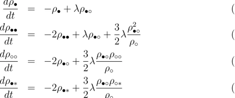
and summing over all processes, we obtain dρ•

dt = −ρ•+λρ•◦ (3.12)

dρ••

dt = −2ρ••+λρ•◦+ 3 2λ

ρ2

•◦

ρ◦

(3.13) dρ◦◦

dt = −2ρ•◦+ 3 2λ

ρ•◦ρ◦◦

ρ◦

(3.14) dρ•∗

dt = −2ρ•∗+ 3 2λ

ρ•◦ρ◦∗

ρ◦

(3.15)

where some variables were eliminated using equations (3.10) and (3.11). After some algebra we obtain the following equation for the stationary density,

(32)

x 0.02 0.05 0.1 0.2 0.3 0.35 MFT 0.020 0.053 0.111 0.250 0.428 0.538 Simulations 0.022 0.056 0.119 0.278 0.498 0.649

Table 3.1: The ratio[λc(x)−λc(0)]/λc(0)for critical parameters obtained through

mean-field theory and simulations.

+ 16(1−x)2+ 12λ(3x−2x2 −ρ∗∗+ρ∗∗x−1) = 0. (3.16)

Solving Eq. (3.16) forρ_• and setting ρ_• = 0, we get

λc(x) =

4(1−x) 3(1−2x+ρ∗∗)

. (3.17)

By settingx= 0 we recover the pair-approximation result for the regular CP, λc(0) =

4/3. Since sites are removed independently, ρ∗∗=x2, and Eq. (3.17) becomes

λc(x)

λc(0)

= 1

(1−x). (3.18)

Thus the relative shift in the critical point [λc(x)− λc(0)]/λc(0) shows the same

dependence on dilution concentration in both the site- and pair-approximations. This suggests that Eq. (3.18) may provide a reasonable estimate. In table 3.1 the shifts [λc(x)−λc(0)]/λc(0) are listed for different dilution concentrations. As we can see

there is fair agreement between simulation and MFT, as long as 1−x is well above the square-lattice site percolation threshold,pc≃0.5927. (Simple mean-field theories

do not detect the breakdown of connectivity for 1−x < pc.)

3.4 Discussion

It is well-known that mean-field cluster expansions generally provide qualitatively cor-rect descriptions of phase diagrams. Based on our results, cluster expansions predict a continuous absorbing-state transition in the diluted contact process atλc(x). They

yield a critical parameter that depends on the dilution,x. In fact a similar result was also found by Marques [25] in a mean-field renormalization group study of the effects of dilution on the contact process and related models. (Marques considers a diluted model slightly different from ours). We believe that the relation,λc(x)∼λc(0)/(1−x),

(33)

0 0.5 1 1.5 2

pc 0.7 0.8 0.9 1

λc(x)/λc(0)

1−x

✸ ✸ ✸ ✸ ✸

✸ ✸

Figure 3.3: λc(x)/λc(0) versus (1−x); the full curve represents the mean-field results,

and the ✸ the simulation values.

as long asx <<1−pc. A plot ofλc(x)/λc(0) versus (1−x), Fig. (3.3), for simulation

and mean-field results, support this conjecture. Dilution has the effect of increasing the critical parameter; this increase is the way the system balances the creation inhi-bition caused by removing sites from the lattice, consequently reducing the number of effective neighbors. On the other hand, this technique yields poor quantitative results for critical exponents. This is expected to happen as we neglect correlations in systems that are highly correlated.

From Fig. (3.3) we notice that the critical parameter,λc, for the contact process

on a percolation cluster (1−x =pc) is finite. Indeed, the critical parameter λc(x=

1−pc) must be less than or equal to λc(x = 0) for the one-dimensional contact

process. This happens as a consequence of the strong dependence of the critical parameter on the number of occupied neighbors. In one dimension, sites have but two occupied neighbors, while in the backbone of an incipient percolation cluster, lots of sites might have more than two occupied neighbors. Thus, the critical parameter of the one-dimensional CP serves as an upper limit for the CP in the percolation cluster (λc(x= 1−pc)≤3.29771) [27].

(34)

(35)

Chapter 4 Diluted Contact Process

-Simulations

4.1 Introduction

The present chapter is best viewed as a continuation of the previous one. Here we study the diluted contact process via numerical methods. We obtain the critical parameter and exponents pertinent to critical behavior through Monte Carlo simula-tions. Numerical simulations have been shown to be very useful in the understanding of nonequilibrium phase transitions, exact solutions are generally impossible, and very laborious in the rare instances where they are feasible. As we will see, simulations are not straightforward either, and require a number of tricks in order to provide accurate results.

We start this chapter by describing the diluted contact process (DCP) in its discrete version. In section (4.3) we consider simulations of the steady-state behav-ior. Then we study the time-dependent properties in section (4.4). In section (4.5) we review the nonexponential relaxation to the vacuum of the survival probability. Concluding remarks are presented in section (4.6).

4.2 The Model

(36)

differ somewhat at short times, but they share the same stationary properties and long-time dynamics. In the discrete version one step consists of first choosing a site randomly. Then if it is occupied either of the processes may take place: annihilation with probability 1/(1 +λ), or creation at a randomly chosen nearest neighbor (if it is vacant), with probability λ/(1 +λ). If the site chosen initially is vacant, nothing happens. After each step (successful or not) time is advanced by a fixed increment, ∆t. (It is conventional to set ∆t = 1/N, where N is the total number of sites, since this implies an average of one event per site, per unit time). A great improvement in efficiency is obtained by choosing from a list of occupied sites. This avoids the waste of time associated with the large proportion of rejected trials, when the density of particles is low. When the initial site is chosen from the list of allNocc occupied sites,

the time increment should be defined as ∆t = 1/Nocc.

We introduce disorder by randomly removing a fraction xof the sites. That is, for each (i, j)∈Z2 _{there is an independent random variable}_{η(i, j), taking values 0 and}

1 with probabilityx and 1−x, respectively. The DCP is simply the contact process restricted to sites with η(i, j) = 1; sites with η(i, j) = 0 may never be occupied. Naturally, 1−xmust exceed the percolation thresholdpc= 0.5927 for there to be any

possibility of an active state, since on any finite set the CP is doomed to extinction. Each trial is generated as follows. We first initialize the lattice by randomly removing sites accordingly to a preset dilution. Then we define an initial particle distribution which depends on the kind of properties we intend to study. We let the process evolve, annihilation and creation of particles take place, until a maximum time tmax. Once this trial is complete, we start a new one by setting the same initial

particle distribution, but generating a new set of disorder. An independent realization of disorder (the variables η(i, j)), is generated for each trial, and thus we perform an average over disorder. As critical points are characterized by power-law divergencies of the correlation length and the relaxation time, one has to study large systems over long times to obtain reliable results.

4.3 Steady-state Behavior

(37)

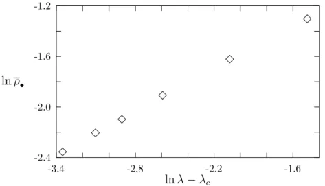
-2.4 -2.0 -1.6 -1.2

-3.4 -2.8 -2.2 -1.6

lnρ•

lnλ−λc

✸

✸ ✸ ✸

Figure 4.1: Log-log plot of the stationary density vs. (λ−λc) for x= 0.02.

according to its dynamics until, after a relaxation timeτ, the steady state1 _{is reached.}

Once in the steady state one measures the density of particles (ρ_•, where the bar indicates a stationary value) at various time intervals up to tmax thus performing a

time average. As we have seen, the density of particles in the active state goes to zero whenλ →λc+ as

ρ• ∼∆β, (4.1)

where ∆≡λ−λc and β is the critical exponent associated with the order parameter.

Log-log plots of the order parameter versus ∆ should provide a straight line whose slope is the critical exponentβ.

4.3.1 Simulation Results

The results for ρ_• were obtained by averaging over typically 50 to 100 independent samples. The number of time stepst and system sizes Lvaried fromt= 1000, L= 32 far from λc to t = 6000, L = 128 to closest to λc. To evaluate ∆ we must of course

have an accurate value ofλc(x); in this study we use the values given in Table 4.2. In

section (4.4) we explain the method we use to determine the critical parameters. In Fig. (4.1) we plot ρ_•×∆ for x= 0.02, and using λc= 1.6850(3). It is clear

from this picture that the power-law behavior of eq. (4.1) is confirmed. Furthermore, it can also be taken as a confirmation that λc = 1.6850(3) marks a critical point.

1_{Instead of steady state, we would rather use “quasi-steady state” as the system only attains an}

(38)

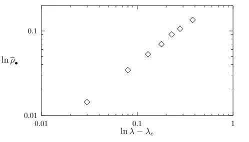
0.01 0.1

0.01 0.1 1

lnρ•

lnλ−λc

✸

✸ ✸

✸ ✸✸

✸

Figure 4.2: Log-log plot of ρ_• vs. (λ−λc) forx= 0.35.

We estimate β = 0.566(7) where the figure in parenthesis indicates the estimated uncertainty in the last digit. This result for β is in good agreement with the typical estimates for directed percolation in (2 + 1) dimensions,β = 0.586(14) [54]. Following the same procedure, we estimateβ = 0.89(1) for x= 0.35, as shown in Fig. (4.2).

4.4 Time-dependent Behavior

4.4.1 Scaling Ansatz

We consider from now on asymptotic distributions of configurations starting off at t = 0 with one particle at the origin. In the scaling regime, i.e., very close to the critical point, at long times and in large systems, there is a unique dominant length scale ξ and time scale τ. According to the scaling hypothesis, one expects that properties such as the local density ρ•(x, t) or the survival probability P(t), depend

on the relevant parameters x, t and ∆, only through the scaling variables x2/tz _and

∆t1/νk_{, times some power of}_x2_{, t}_{or ∆. The dependence on position,}_{x, is demanded by}

symmetry and the growth of the characteristic length scale∝tz/2 _{(note however that}

z is not the critical exponent of dynamic critical phenomena); the time-dependence involves the ratio t/τ, since τ ∝ ∆−νk _{[13]. Thus, in the scaling regime, the local}

particle density, averaged over all trials, surviving or not, can be written as

(39)

and for the survival probability, the probability that the system has not reached the absorbing state at timet, we expect

P(t)≃t−δ_φ(∆t1/νk_). _(4.3)

η and δ are further critical exponents, while F and φ are scaling functions. Using Eq. (4.2), we get for the mean number of particlesn(t) and the mean-square distance of spreading R2_(t),

n(t) =

Z

ddxρ•(x, t)∝tηf(∆t1/νk),

R2(t) = 1 n(t)

Z

ddxx2ρ•(x, t)∝tzg(∆t1/νk). (4.4)

From eqs.(4.3) and (4.4) it is easy to see that if the functions φ(y), f(y) and g(y) are nonsingular at y = 0, the asymptotic behavior of P(t), n(t) and R2_{(t) as} _t _{→ ∞, at}

the critical point, determines the critical exponentsδ, η and z: P(t)∝ t−δ_,

n(t)∝ tη_,

R2(t)∝ tz_. _(4.5)

The asymptotic behavior of the scaling functions for ∆t1/νk _{→ −∞} _{is obtained by}

noting that far from the critical point correlations are short-ranged. Thus, in the subcritical region, λ < λc, P(t) and n(t) decay exponentially, while R2(t) ∝ t, as if

particles diffused on the lattice. In the supercritical regime, λ > λc, there must be

a nonzero chance of survival, P∞ ≡ limt→∞P(t)> 0; the active region expands into

the vacuum at a constant rate, so thatn(t)∝td_in_d_{dimensions and}_R2_(t)_∝_t2_{. Still}

considering the ∆>0 region, we see that by settingψ(ζ) = ζ−δνk_{φ(ζ) we may rewrite}

eq. (4.3) as

P(t)∝∆δνk_ψ(∆t1/νk_). _(4.6)

SinceP∞ is finite, limζ→∞ψ(ζ) is finite too, and we get P∞ ∼∆δνk. It can be shown

that the ultimate survival probability and the stationary particle density have the same critical exponent [22]. Hence as ρ• ∝ ∆β, we must have the following scaling

relation

(40)

Let us consider next the local density at any fixed x. In the limit t → ∞ and for ∆>0,

ρ•(x, t)→P∞ρ• ∝∆2β, (4.8)

sinceρ•(x, t) in eq. (4.2) represents the density averaged over all trials. From eq. (4.2)

we see that F(0,∆t1/νk)∝∆2βt2β/νk, for ∆t1/νk large and positive. Thus we get

ρ•(x, t) =tη−dz/2∆2βt2β/νk. (4.9)

In order to remove the overallt-dependence we must have

4δ+ 2η=dz, (4.10)

where we used β = δνk. This expression is known as the hyperscaling relation as it

relates the dimensionality to critical exponents. It is expected to hold for d ≤ dc.

Further scaling relations among critical exponents can be found in [13].

4.4.2 Simulation Results

We studied dilutionsx= 0.02, 0.05, 0.1, 0.2, 0.3, and 0.35, on square lattices of 2200 sites to a side, using samples of from 104 _{to 2}_×₁₀6 _{trials for each}_λ _{value of interest,}

each trial extending to a maximum time of tmax ≤ 2×106. As is usual in this sort

of simulation, the time increment associated with an elementary event — creation or annihilation — is ∆t = 1/N, whereN is the number of particles. The largest samples and longest runs were used at or near critical. An independent realization of disorder (the variablesη(i, j)), is generated for each trial.

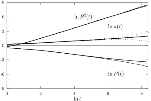
In Fig. (4.3) we show log-log plots ofP(t), n(t) andR2_{(t), as functions of}_t _for

dilutionx= 0.02. The plot illustrates these quantities at both critical and off-critical values. Forλ= 1.68 we see thatn(t) and P(t) show a negative curvature, indicating that this parameter is subcritical. In the same way, we see a positive curvature for the supercritical value λ = 1.69. The power-law behavior as predicted by eq. (4.5) at the critical point is found for λ = 1.685. Notice that the plot for n(t) is more sensitive to the changes in λ, showing a more pronounced curvature for the sub and supercritical parameters. We will see that the same is true for the local slope plots. A more accurate determination of the critical point is afforded by analyzing the local slopesδ(t),η(t), andz(t) which are given by

−δ(t) = ln[P(t)/P(t/m)]

(41)

-9 -6 -3 0 3 6 9

0 2 4 6 8

lnt

lnP(t) lnn(t) lnR2_(t)

Figure 4.3: Log-log plots of P(t), n(t) and R2_(t) _versus _t _for _x _{= 0.02}_{. In each plot,}

from bottom to top, we haveλ= 1.68; 1.685; 1.69.

where m is a fixed integer. Analogous expressions hold for η(t) and z(t). In the present work we compute the local slopes by using least-squares fits to the data (in a logarithmic plot), distributed symmetrically about a givent (typically in the interval [t/3, 3t]). We estimate the exponents by plotting the local slopes versus 1/t and extrapolating to 1/t → 0 [8]. In Fig. (4.4) we plot the corresponding local slopes for x = 0.02. In plots of the local slopes versus 1/t one sees that the curves for the off-critical values ofλ veer up or down, in the supercritical or subcritical regime, respectively. We estimate the critical parameter λc for x = 0.02 by looking at the

curvature of theη(t) andδ(t) plots. Both yield the best estimateλc= 1.685(5). More

detailed results indicate thatλc(x= 0.02) is in fact 1.6850(3), see Table 4.2. For the

critical exponents we get δ= 0.467(1);η= 0.216(3); andz = 1.104(2).

For dilution x = 0.02 the DCP exhibits a pure-CP behavior even at very long times. The same is not true when considering a higher degree of disorder. In Fig. (4.5) we plot P(t), n(t) and R2_{(t) as a function of} _t _{(in a logarithmic scale) for}

(42)

-0.5 -0.47 -0.44

0.03 0.05 0.07 0.09

−δ 1/t ✸ ✸ ✸ ✸ ✸ ✸ ✸ ✸ ✸ ✸ ✸ ✸ ✸ ✸ + + + + + + + + + + + + + + ✷ ✷ ✷ ✷ ✷ ✷ ✷ ✷ ✷ ✷ ✷ ✷ ✷ ✷ × × × × × × × × × × × × × × 0.15 0.18 0.21 0.24

0.03 0.05 0.07 0.09

η 1/t ✸ ✸ ✸ ✸ ✸ ✸ ✸ ✸ ✸ ✸ ✸ ✸ ✸ ✸ + + + + + + + + + + + + + + ✷ ✷ ✷ ✷ ✷ ✷ ✷ ✷ ✷ ✷ ✷ ✷ ✷ ✷ × × × × × × × × × × × × × × 1.1 1.13 1.16

0.03 0.05 0.07 0.09

z 1/t ✸ ✸ ✸ ✸ ✸ ✸ ✸ ✸ ✸ ✸ ✸ ✸ ✸ ✸ + + + + + + + + + + + + + + ✷ ✷ ✷ ✷ ✷ ✷ ✷ ✷ ✷ ✷ ✷ ✷ ✷ ✷ × × × × × × × × × × × × × ×

(43)

-10 -5 0 5 10 15

0 5 10 15

lnt lnP

lnn lnR2

Figure 4.5: Plots of the survival probabilityP(t), mean number of particles n(t) and the mean-square distance of particles from the origin R2_(t) _versus _t_{, in the diluted contact}

process forx= 0.3. In each plot, from bottom to top, we have λ = 2.40;λ= 2.47; and

λ= 2.50.

may be given as follows (a more complete discussion is given in the next section). The probability of the seed landing in a favored region, of linear sizeL, in which the local density of diluted sites is such that λ−λc,ef f = ∆, is ∼ exp(−ALd). (λc,ef f is the

critical creation rate for a system with the site density prevailing in this region.) The lifetime of the process in such a region is proportional to ∼ exp(BLd_{). (The precise}

forms of A and B are unknown, but it is clear that they are positive, increasing functions of ∆ for ∆>0.) It follows that at long times

P(t)∼max∆,Lexp[−(ALd+te−BL)]∼max∆t−A/B ∼t−φ, (4.12)

where the last step defines a (nonuniversal) decay exponentφ. In fact, from Fig. (4.5), we see that this is the case forλ = 2.40 which is subcritical. In order to identify the critical curve we use the following criteria. It is known that the survival probability in the supercritical regime approaches a nonzero value, the ultimate survival probability P∞, at asymptotic times. Thus if P(t) attains a plateau at later times, as for λ =