The identification and tracking of volcanic ash using the Meteosat Second Generation (MSG) Spinning Enhanced Visible and Infra-Red Imager (SEVIRI)

(1)

AMTD

6, 5577–5619, 2013

The identification of volcanic ash using

the MSG SEVIRI

A. R. Naeger and S. A. Christopher

Title Page

Abstract Introduction

Conclusions References

Tables Figures

◭ ◮

Back Close

Full Screen / Esc

Printer-friendly Version Interactive Discussion

Discussion

P

a

per

|

Di

scussion

P

a

per

|

Discussion

P

a

per

|

Discussi

on

P

a

per

|

Atmos. Meas. Tech. Discuss., 6, 5577–5619, 2013 www.atmos-meas-tech-discuss.net/6/5577/2013/ doi:10.5194/amtd-6-5577-2013

Atmospheric Measurement

Techniques

Open Access

Discussions

Geoscientiic Geoscientiic

This discussion paper is/has been under review for the journal Atmospheric Measurement Techniques (AMT). Please refer to the corresponding final paper in AMT if available.

The identification and tracking of volcanic

ash using the Meteosat Second

Generation (MSG) Spinning Enhanced

Visible and Infra-Red Imager (SEVIRI)

A. R. Naeger1and S. A. Christopher1,2

1

Department of Atmospheric Sciences, UA Huntsville, 320 Sparkman Drive, Huntsville, AL 35805, USA

2

Earth System Science Center, UA Huntsville, 320 Sparkman Drive, Huntsville, AL 35805, USA

Received: 10 May 2013 – Accepted: 11 June 2013 – Published: 21 June 2013 Correspondence to: A. R. Naeger ([email protected])

(2)

AMTD

6, 5577–5619, 2013

the MSG SEVIRI

Title Page

Tables Figures

◭ ◮

Back Close

Full Screen / Esc

Discussion

P

a

per

|

Di

scussion

P

a

per

|

Discussion

P

a

per

|

Discussi

on

P

a

per

|

Abstract

In this paper, we develop an algorithm based on combining spectral, spatial, and tem-poral thresholds from the geostationary Spinning Enhanced Visible and InfraRed

Im-ager (SEVIRI) daytime measurements to identify and track di_fferent aerosol types,

pri-marily volcanic ash. Contemporary methods typically do not use temporal information

5

to identify ash. We focus not only on the identification and tracking of volcanic ash dur-ing the Eyjafjallajökull volcanic eruption period beginndur-ing 14 April 2010 to May but a pixel level classification method for separating various classes in the SEVIRI images. Three case studies on 19 April, 16 May, and 17 May are analyzed in extensive detail with other satellite data including the Moderate Resolution Imaging

Spectroradiome-10

ter (MODIS), Multi-angle Imaging Spectroradiometer (MISR), Cloud-Aerosol Lidar and Infrared Pathfinder Satellite Observations (CALIPSO), and Facility for Airborne Atmo-spheric Measurements (FAAM) BAe146 aircraft data to verify the aerosol spatial distri-bution maps generated by the SEVIRI algorithm. Our results indicate that the SEVIRI algorithm is able to track volcanic ash even at these high latitudes. Furthermore, the

15

BAe146 aircraft data shows that the SEVIRI algorithm detects nearly all ash regions

when AOD>_{0.2. However, the algorithm has higher uncertainties when AOD is}<_0.1

over water and AOD<_{0.2 over land. The ash spatial distributions provided by this}

algo-rithm can be used as a critical input and validation for atmospheric dispersion models simulated by Volcanic Ash Advisory Centers (VAACs). Identifying volcanic ash is an

20

important first step before quantitative retrievals of ash concentration can be made.

1 Introduction

The Eyjafjallajökull volcano located on the southern coast of Iceland (63.6◦N, 19.6◦W)

began emitting ash into the atmosphere on 14 April 2010. Although only a mid-size eruption (Mason et al., 2004; Mastin et al., 2009), the volcano had a tremendous

im-25

(3)

AMTD

6, 5577–5619, 2013

the MSG SEVIRI

Title Page

Tables Figures

◭ ◮

Back Close

Full Screen / Esc

Discussion

P

a

per

|

Di

scussion

P

a

per

|

Discussion

P

a

per

|

Discussi

on

P

a

per

|

towards Europe (Ansmann et al., 2010a). By 16 April 2010, a dense ash plume was observed across Central Europe by Aerosol Robotic Network (AERONET) Sun pho-tometers and ground based lidars (Ansmann et al., 2010b). The presence of dense ash caused nearly a week-long stoppage in air travel over many parts of Europe. Flight cancellations that occurred over the ensuing week proved extremely costly to the

air-5

line industry as monetary losses were over 1 billion US dollars. Also, the damaging

effects of volcanic ash on commercial airplanes can be deadly due to their low melting

temperature and sharp-edged shapes (Casadevall, 1992). Therefore, it is critical that we accurately track volcanic ash during an eruption period.

To track the spatial distribution of volcanic ash, satellite remote sensing is important

10

as the spatial distribution of ash varies strongly especially after an eruption. Ground based stations are inadequate for understanding the spatial distribution as they only provide point measurements. Satellites are also an important tool for verifying mod-els that predict ash concentrations and spatial distributions (Millington et al., 2012). These models are usually high resolution dispersion models that predict height

depen-15

dent ash concentrations used by Volcanic Ash Advisory Centers (VAACs). Although polar orbiting satellites such as the Moderate Resolution Imaging Spectroradiometer (MODIS) can provide high spatial resolution of volcanic ash plumes (Sigmundsson et al., 2010), their temporal resolution is insufficient to track ash plumes being transported long distances over relatively short time scales. Thus, geostationary satellite sensors

20

such as the Spinning Enhanced Visible and InfraRed Imager (SEVIRI) are critical for assessing the spatial distributions of ash due to their high temporal resolutions (Prata and Kerkmann, 2007; Christopher et al., 2012).

Ultimately it is important to know the vertical distribution of ash concentrations be-fore important decisions can be made regarding commercial flights during eruptions.

25

(4)

AMTD

6, 5577–5619, 2013

the MSG SEVIRI

Title Page

Tables Figures

◭ ◮

Back Close

Full Screen / Esc

Discussion

P

a

per

|

Di

scussion

P

a

per

|

Discussion

P

a

per

|

Discussi

on

P

a

per

|

spatial coverage make SEVIRI an excellent tool for mapping volcanic ash over large areas. The common method is to simply assign separate channels to the Red, Green, and Blue and visually examines the ash by looking for certain colors. This is often problematic since clouds can be confused as ash and not all aerosols appear to have the same color; and therefore, it is important to develop an algorithm that separates

5

an image into various classes, such as cloud and aerosol, for further studies that may involve calculation of ash concentrations.

Prata (1989) presented a very commonly used technique that exploits the brightness

temperature difference (BTD) between the 11 and 12 µm channels. The limitations with

this simple technique are well known and discussed in Prata et al. (2001) where one

10

major limitation is that high water vapor amounts can mask the negative BTD signal which the technique relies on ash detection. Pergola et al. (2004) developed a more sophisticated ash detection technique that compares a measured satellite signal to a reference field computed from long-term historical records. In particular, they use three channels centered at approximately 3.75, 11.0, and 12.0 µm from the Advanced

15

Very High Resolution (AVHRR) to compute the reference fields and they show that this Robust AVHRR Technique (RAT) is more accurate in detecting volcanic ash than the simple BTD technique presented in Prata (1989). However, this approach requires mul-tiple years of data over a region to compute the reference fields. Pavolonis et al. (2006) developed a four channel ash detection algorithm that utilizes the 0.65, 3.75, 11.0,

20

and 12.0 µm channels and does not rely on a reference field but instead uses spectral tests and a spatial filtering routine. They showed that this four channel algorithm is much better at detecting volcanic ash regions compared to the BTD approach with less

false detections. We take a different approach by developing an algorithm using

SE-VIRI measurements that exploits temporal thresholds along with spectral and spatial

25

thresholds to classify each pixel into various classes (e.g., cloud, land, and aerosol).

This algorithm uses seven different SEVIRI channels to produce detailed spatial

(5)

AMTD

6, 5577–5619, 2013

the MSG SEVIRI

Title Page

Tables Figures

◭ ◮

Back Close

Full Screen / Esc

Discussion

P

a

per

|

Di

scussion

P

a

per

|

Discussion

P

a

per

|

Discussi

on

P

a

per

|

Although the SEVIRI instrument is not equipped with near ultraviolet (UV) channels, it is important to note the ability of the near-UV channels in detecting volcanic ash. Torres et al. (1998) used the near-UV channels of 340 and 380 nm from the Total Ozone Mapping Spectrometer (TOMS) instrument to detect volcanic ash, and they found that these two channels have great success in detecting ash over snow/ice or above clouds.

5

This is an important advantage of using the near-UV channels as detection techniques using channels from the visible to infrared spectrums, such as the RAT and our SEVIRI algorithm, do not possess the same capability of detecting ash over snow/ice or above clouds (Pergola et al., 2004). In addition, Krotkov et al. (1999) showed that the near-UV channels of the TOMS instrument can detect the optically opaque, very fresh ash

10

which is often missed by the visible and infrared techniques.

This study tracks the ash plumes emitted from the Eyjafjallajökull volcano from its initial eruption on 14 April until the end of the eruption period on 23 May using the high temporal resolution measurements of SEVIRI onboard the Meteosat Second Gener-ation (MSG-2) satellite. Since we use the visible along with the infrared channels of

15

SEVIRI, the algorithm developed in this study can only track the ash plumes during the daylight periods for volcanic ash in cloud-free conditions. We present results from the SEVIRI algorithm throughout the eruption period but place special emphasis on six days in May 2010 when the Facility for Airborne Atmospheric Measurements (FAAM) BAe146 research aircraft measurements was available (Johnson et al., 2012). We use

20

the FAAM BAe146 aircraft measurements as validation for the SEVIRI algorithm de-veloped in this study. Other sources of verification data used in this study to assess the spatial distribution of the aerosols detected by the SEVIRI algorithm include the MODIS, the Multi-angle Imaging SpectroRadiometer (MISR), and the Cloud-Aerosol Lidar and Infrared Pathfinder Satellite Observation (CALIPSO).

(6)

AMTD

6, 5577–5619, 2013

the MSG SEVIRI

Title Page

Tables Figures

◭ ◮

Back Close

Full Screen / Esc

Discussion

P

a

per

|

Di

scussion

P

a

per

|

Discussion

P

a

per

|

Discussi

on

P

a

per

|

2 Data

The goal of the paper is to develop a pixel level algorithm from SEVIRI reflectance and temperature measurements using temporal threshold tests along with spatial and spectral threshold tests. It is important to note that the retrieval of ash concentrations and aerosol particle size information is beyond the scope of this study. We have

al-5

ready noted that the use of temporal thresholds and some of the spatial thresholds used in this paper is not routinely done by standard algorithms (i.e., Prata, 1989). After classifying the volcanic ash pixels, we need to determine the accuracy of the algorithm

but this is a difficult task to accomplish. We have chosen to intercompare the SEVIRI

algorithm results with MODIS and MISR products by making the assumption that their

10

identification is correct. We take this a step further by comparing our results with air-craft data but not many data points can be obtained with such a comparison. This is not a unique problem to our study since all validation methods have to use a verification source and then provide results and analysis.

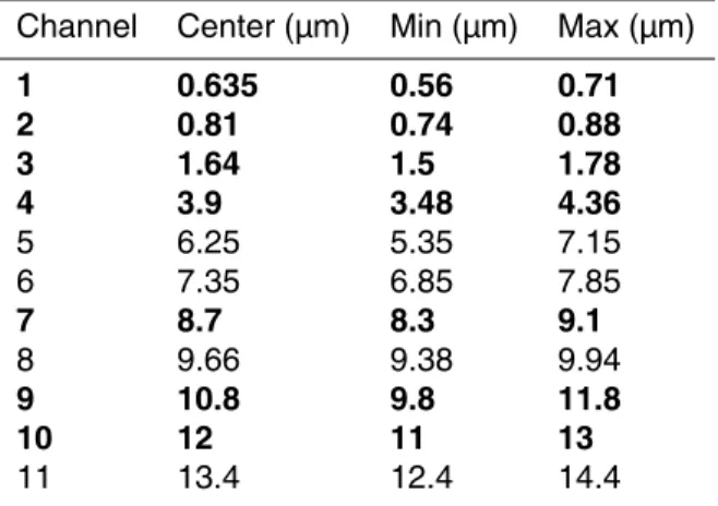
Table 1 shows the SEVIRI channels with the center, minimum, and maximum

wave-15

lengths for each channel. These channels have a sampling distance of 3 km at sub-satellite point (Schmetz et al., 2002). The channels used to develop the SEVIRI algo-rithm are highlighted while the channels ignored are primarily used for water vapor, ozone, and carbon dioxide detection. Thus, the SEVIRI algorithm uses three channels in the solar spectrum and four channels in the infrared spectrum.

20

The MODIS onboard the Terra and Aqua polar orbiter satellites have 36 channels over the spectral range from 0.4–14.4 µm with spatial resolutions of 250 m, 500 m, and 1 km (Savtchenko et al., 2004). A Level 2 aerosol optical thickness (AOT) operational product over both ocean and non bright land surfaces is provided by MODIS at a spa-tial resolution of 10 km (at nadir) by comparing measured reflectances to a lookup

25

table of computed reflectances from a radiative transfer model (Remer et al., 2005).

The reported uncertainties over ocean and non bright surfaces are±0.03±0.05τand

(7)

AMTD

6, 5577–5619, 2013

the MSG SEVIRI

Title Page

Tables Figures

◭ ◮

Back Close

Full Screen / Esc

Discussion

P

a

per

|

Di

scussion

P

a

per

|

Discussion

P

a

per

|

Discussi

on

P

a

per

|

et al., 2005). Additionally, the MODIS Deep Blue Algorithm provides AOT values over deserts and other bright surfaces where the reported uncertainties are approximately 20–30 % (Hsu et al., 2006). The Multi-angle Imaging SpectroRadiometer (MISR) in-strument onboard the Terra satellite measures upwelling shortwave radiance in four spectral channels (446, 558, 672, and 867 nm) with nine view angles and spatial

reso-5

lutions of about 250 m to 1.1 km. To produce the MISR Level 2 product (MIL2SAE, F12,

22) with a spatial resolution of 17.6 km, top-of-atmosphere radiances from 16×16 pixel

areas of 1.1 km resolution are analyzed (Diner et al., 1999). The multispectral and mul-tiangle instrument retrieves accurate AOT values, even over bright deserts (Christopher

and Wang, 2004; Kahn et al., 2005), with expected uncertainties of±0.05 for AOT<0.5

10

and±10 % for AOT>0.5 (Martonchik et al., 1998). We use the aerosol spatial

distribu-tion from MODIS and MISR to help verify the SEVIRI results that we have developed in this paper.

The CALIPSO satellite flies in formation with the “A-Train” constellation of satellites that also includes the Aqua-MODIS used in this study (Stephens et al., 2002). The

15

Cloud-Aerosol Lidar with Orthogonal Polarization (CALIOP) onboard the CALIPSO satellite measures polarization-sensitive backscatter vertical profiles at 532 and 1064 nm during the day and night at a resolution of 333 m (Vaughan et al., 2004). The backscatter vertical profiles give information on the location of clouds and aerosols in the atmosphere as they are associated with higher backscatter values than the clear

20

sky background. The color ratio (1064/532 nm total attenuated backscatter) and depo-larization ratio (perpendicular/parallel channels at 532 nm) profiles are computed from the backscatter measurements which helps separate clouds from aerosols. After locat-ing cloud and aerosol layers by uslocat-ing the Selective, Iterated Boundary Locator (SIBYL), CALIPSO produces a vertical feature mask (VFM) product (Level 2, Version 3.1) that

25

shows the spatial distribution of clouds and aerosols in the atmosphere (Liu et al., 2010). We use the CALIPSO VFM product for verifying the SEVIRI algorithm.

(8)

AMTD

6, 5577–5619, 2013

the MSG SEVIRI

Title Page

Tables Figures

◭ ◮

Back Close

Full Screen / Esc

Discussion

P

a

per

|

Di

scussion

P

a

per

|

Discussion

P

a

per

|

Discussi

on

P

a

per

|

355 nm Lidar, the Passive Cavity Aerosol Spectrometer Probe (PCASP), and the Cloud and Aerosol Spectrometer (CAS) (Marenco et al., 2011). The FAAM BAe146 aircraft flew on six days in May 2010 where aerosol extinction and AOTs at 355 nm were retrieved along with ash mass concentrations and size distributions (Marenco et al., 2011). This study focuses on 16 May and 17 May since the volcanic ash was

associ-5

ated with higher AOTs on these days. We utilized the AOT measurements at 355 nm retrieved from the lidar which samples the atmosphere from 2 km above the surface to 300 m below the aircraft. Thus, the lidar AOTs exclude any boundary layer contribution, except for the 17 May case where boundary layer aerosols contribute less the 0.05 to the AOT. After integrating the AOT measurements over every minute, each retrieved

10

AOT value corresponded to an along-track distance of 8–10 km. Note that AOT can still be derived in the presence of clouds by using the instruments onboard the BAe146 aircraft to detect and mask the cloud contaminated areas in the vertical column of air beneath the aircraft. The usefulness of BAe146 aircraft measurements has been shown in a number of papers where the aircraft measurements were analyzed along

15

with satellite measurements (Johnson et al., 2012; Christopher et al., 2009; Naeger et al., 2013).

3 Methodology

There is a rich heritage of classification algorithms with the most common ones using

the concept of spectral signatures where for example clouds “look different” based on

20

spectral signatures in some wavelengths when compared to aerosols and land. A clas-sic paper by Saunders and Kriebel (1988) used spectral and some spatial signatures to separate pixels into cloud-free, partly cloudy, or overcast scenes. Using spectral thresholds alone can cause uncertainties in image classification since there could be spectral overlap between and among classes. Thus, it is not possible to accurately

25

(9)

sep-AMTD

6, 5577–5619, 2013

the MSG SEVIRI

Title Page

Tables Figures

◭ ◮

Back Close

Full Screen / Esc

Discussion

P

a

per

|

Di

scussion

P

a

per

|

Discussion

P

a

per

|

Discussi

on

P

a

per

|

arate aerosols from clouds over oceans due to the mean and standard deviation for

a group of aerosol pixels being different than clouds. Spatial measures are a form of

texture identification where a group of aerosol pixels appear different than clouds due

to several measures and one example being their homogeneity. Therefore, combining spectral and spatial information reduces the frequency of misclassifications within an

5

image.

In this paper, we take this a step further by using temporal information along with spectral and spatial information as the high temporal resolution of geostationary satel-lite sensors permits the use of these tests, but only a handful of studies have actu-ally used temporal tests (Calle et al., 2006; de Wildt et al., 2007). Calle et al. (2006)

10

proposed a fire detection technique that utilized temporal information from the 3.9 µm SEVIRI channel and showed that false alarm rates were lower than when detecting fires without using any temporal information. Typically the temperature from the 3.9 µm channel does not encounter large variations with time, but Calle et al. (2006) found that large increases occur with the onset of fires which helps better detection of fires.

15

Cloud detection can also be improved when using temporal information since the tem-poral variation of the reflectance and temperature of a pixel is usually greatly impacted by the presence of clouds. For example, when analyzing the reflectance of the 0.6 µm SEVIRI channel for a pixel over a period of time, the variation in the reflectance will be minimal in most clear sky cases but rather large for most cases where clouds are

20

present since clouds are typically much more heterogeneous than the underlying land surface. Then, de Wildt et al. (2007) developed temporal tests using reflectance and temperature channels from SEVIRI and found that these tests helped mask clouds and cloud shadows which ultimately led to more accurate detection of snow cover. Although the temporal tests detected most clouds due to their heterogeneity, they had to rely on

25

(10)

AMTD

6, 5577–5619, 2013

the MSG SEVIRI

Title Page

Tables Figures

◭ ◮

Back Close

Full Screen / Esc

Discussion

P

a

per

|

Di

scussion

P

a

per

|

Discussion

P

a

per

|

Discussi

on

P

a

per

|

may be cloud free in the current time-step but cloudy in the previous one. This situ-ation can cause a significant increase in the varisitu-ation of reflectance and temperature with time for a cloud free pixel. Therefore, even though temporal techniques have been used successfully for detecting fires and clouds, they also encounter problems that are investigated further in this study.

5

3.1 General flow of algorithm

For our algorithm, we first identify pixels that are land (or over land) and pixels that are

water (or over water) to make the algorithm efficient and save computational time. This

is necessary since the thresholds used to identify aerosols and clouds are different

over water than over land. Classification methods are usually easier over water since

10

water has a low visible reflectance and warmer infrared temperatures when compared to aerosols and clouds. However, over land spectral tests pose challenges since the surface reflectance and temperatures can be highly variable. After separating land and water pixels, we then identify cloudy pixels through a series of spectral threshold tests which are labeled as cloud and no longer processed by the algorithm. It is critical to

15

identify cloud pixels because the final goal of this algorithm is to label all cloud-free aerosol pixels. All non-cloud pixels undergo further processing as we identify feature pixels through a series of threshold tests involving both spectral and temporal tests. Feature pixels are simply pixels that are contaminated with any type of aerosol or cloud. Finally, all pixels labeled as feature are fed into the final threshold tests that attempt

20

to identify any remaining clouds through spectral, spatial, and temporal tests. If the feature pixel passes one of these tests, then it is labeled as cloud. If the pixel fails all of these tests, then the pixel is labeled as aerosol. Since the aerosol spatial distribution maps can be produced every 15 min when using SEVIRI, they can provide near real-time information on the location of volcanic ash which is a major aviation concern

25

(11)

AMTD

6, 5577–5619, 2013

the MSG SEVIRI

Title Page

Tables Figures

◭ ◮

Back Close

Full Screen / Esc

Discussion

P

a

per

|

Di

scussion

P

a

per

|

Discussion

P

a

per

|

Discussi

on

P

a

per

|

3.2 Input data for algorithm

The US Geological Survey (USGS) global land cover characteristics database ver-sion 2.0, SEVIRI viewing and solar zenith angles, and the SEVIRI channels highlighted in Table 1 are input into our algorithm. SEVIRI viewing and solar zenith angles are pri-marily used for masking sun glint regions and for removing the solar component from

5

the 3.9 µm channel while the SEVIRI channels provide the critical reflectivity and tem-perature values for each pixel. The USGS global land cover data is used immediately in the algorithm to separate land and water pixels and to find bright (e.g., desert) and non-bright (e.g., vegetation) pixels over land since certain threshold tests are not valid over bright surfaces with high reflectivity. Next, we develop a clear sky reflectance map

10

by finding the minimum top of atmosphere (TOA) 0.6 µm reflectance for each pixel over a two-week period surrounding the time of interest (Jolivet et al., 2008). For example, if analyzing a 13:00 UTC SEVIRI image on 19 April 2010, then we find the minimum 0.6 µm reflectance from 12 April until 26 April at 13:00 UTC for each pixel which gener-ates the clear sky reflectance map. For bright surfaces determined by the USGS global

15

land cover map, we find the highest 10.8 µm temperature during the two week period and then extract the 0.6 µm reflectance from this particular pixel. Dust over desert re-gions can reduce the observed TOA reflectance below the actual clear-sky reflectance since dust is slightly absorbing at 0.6 µm (Patadia et al., 2009). While generating the

minimum 0.6 µm reflectance maps, the standard deviation (σ_{) for the SEVIRI solar}

20

zenith angles (SZA) over the two-week period are computed for each pixel. Theσ_SZA

map is used along with the 0.6 µm clear sky reflectance map in an important threshold test which is discussed later in this section.

3.3 Initial cloud detection tests over land

After generating theσ_{SZA and clear sky reflectance maps, the algorithm begins with}

25

(12)

AMTD

6, 5577–5619, 2013

the MSG SEVIRI

Title Page

Tables Figures

◭ ◮

Back Close

Full Screen / Esc

Discussion

P

a

per

|

Di

scussion

P

a

per

|

Discussion

P

a

per

|

Discussi

on

P

a

per

|

land and water pixels prior to the initial cloud detection tests so that these bright pixels can be ignored throughout the remainder of the algorithm. This ice and snow detection

scheme uses the normalized difference snow index (NDSI), which takes advantage of

snow being more reflective at 0.6 µm than at 1.6 µm (Riggs and Hall, 2004), along with other temporal tests. For all the temporal tests used in Table 2, the standard deviation

5

(σ_{) of three successive 15 min SEVIRI images centered on the current image is}

com-puted for the highlighted channels in Table 1. Temporal tests help reduce the frequency of falsely detected clouds as snow or ice (Riggs and Hall, 2004), and for this study we

use theσ of the 1.6 and 10.8 µm as the reflectance and temperature of snow and ice

which typically vary slowly with time (de Wildt et al., 2007). However, we will not go any

10

further into the specifics of the snow and ice detection scheme because it is not critical to the main goal of the algorithm and the results of this paper.

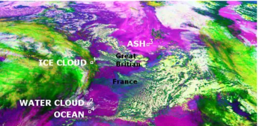
Spectral tests can separate cloud from aerosol and land surfaces due to the diff

er-ing spectral signatures of these features. For example, Fig. 1 is a SEVIRI RGB image on 17 May 2010 at 13:30 UTC over Europe and the Atlantic Ocean where the four

15

boxes indicate the location of extracted samples for ocean, ash, ice cloud, and water cloud. Figure 2a is a wavelength versus reflectivity plot for the three SEVIRI reflectivity channels showing the mean and one standard deviation for the extracted samples in Fig. 1 where the ocean is black, ash is blue, ice cloud is red, and water cloud is pink. Figure 2b is the same as Fig. 2a except wavelength versus temperature for four

SE-20

VIRI temperature channels is displayed. For the reflectivity channels, the water and ice clouds have much higher reflectivity than the ocean while the reflectivity of ash is only about 5–10 % higher than the ocean. Also, the trends across the reflectivity channels is important as the reflectivity increases or stays nearly constant for the water and ice cloud when moving from the 0.6 to 0.8 µm channels while the reflectivity decreases for

25

the ash and ocean pixels. This difference in the trends for these features is due to the

difference in particle sizes and imaginary refractive indices. The mean ash reflectivity

(13)

AMTD

6, 5577–5619, 2013

the MSG SEVIRI

Title Page

Tables Figures

◭ ◮

Back Close

Full Screen / Esc

Discussion

P

a

per

|

Di

scussion

P

a

per

|

Discussion

P

a

per

|

Discussi

on

P

a

per

|

explains the decreasing reflectivity trend for ash across these wavelengths. The much higher water cloud than ice cloud reflectivity at 1.6 µm is due to the higher imaginary refractive indices for ice which means the ice particles absorb more of the incoming ra-diation than water particles leading to lower TOA reflectivity. In Fig. 2b, the much larger temperature decrease from 3.9 to 8.7 µm for ice and water clouds compared to the ash

5

and ocean is due to the added solar reflection component to the 3.9 µm channel. Water and ice particles reflect much of this incoming solar radiation back towards the satellite. The water cloud temperature decrease is larger than that for the ice cloud because the imaginary refractive index for ice is larger than water at 3.9 µm. When analyzing the temperature trend between the 10.8 and 12.0 µm channels, the temperature actually

10

increases with wavelength for ash but decreases for the other features which is due to the unique characteristic of the ash imaginary refractive index being higher at 12.0 than at 10.8 µm causing the slightly lower temperatures at 12.0 µm (Ackerman, 1997). For the spectral threshold tests in Table 2 we used the di_ffering spectral signatures of water, land, cloud, and aerosol to develop the algorithm.

15

The first initial cloud detection test is applied over only bright pixels where a high 0.6 µm reflectance threshold of 60 % is used to detect clouds which ensures that clear sky pixels are not falsely detected as clouds since the highest surface reflectance (i.e., non snow/ice) observed by this study was around 55 % over the Sahara Desert. The second cloud detection test in Table 2 is only applied over non-bright pixels and uses

20

BTD 10.8–12.0>₋_{0.2 K in order to prevent the test from being applied over pixels}

con-taminated with moderate to thick ash that can have reflectivity of 0.6 µm>_{35 %. Thus,}

this test is developed primarily to detect clouds in regions of no ash or thin ash. The BTD 10.8-12.0 technique has been used extensively for both dust and volcanic ash detection as these particular aerosol types have been shown to be associated with

25

(14)

re-AMTD

6, 5577–5619, 2013

the MSG SEVIRI

Title Page

Tables Figures

◭ ◮

Back Close

Full Screen / Esc

Discussion

P

a

per

|

Di

scussion

P

a

per

|

Discussion

P

a

per

|

Discussi

on

P

a

per

|

flectivity>_{50 %. This study found that even the thickest ash regions will typically have}

0.6 µm reflectivity<_{50 % after observing that freshly emitted ash nearby the}

Eyjafjal-lajökull volcano had 0.6 µm reflectivity<_{50 %. Also, note that the moderate ash plume}

over water in Fig. 1 where MODIS retrieved AOD is >_{0.5 only has a 0.6 µm}

reflec-tivity of only about 12 %. The fourth initial cloud detection test is a very simple test

5

that simply labels pixels with 10.8 µm<_{240 K as ice cloud. This test can be confidently}

used in this study since pixels with 10.8 µm<_{240 K are usually snow covered which}

our snow detection scheme has already found. Then, the fifth initial cloud detection test in Table 2 utilizes the BTD between 3.9 and 10.8 µm (BTD 3.9-10.8) which takes

into account the SZA (θ_{) as the 3.9 µm channel is a}_ff_{ected by solar radiation during the}

10

daytime (Christopher et al., 2012; Zhang et al., 2006).

Figure 3 shows bispectral plots for the SEVIRI channels of most interest to this study from the samples in Fig. 1 where ocean is black, ash is blue, ice cloud is red, and water cloud is pink. Figure 3b reveals that the thick ash over water is associated with BTD3.9-10.8 of about 3 K while the ice and water clouds are primarily associated with

15

much larger values. Thus, we use a threshold of BTD 3.9-10.8>_{8 K for cloud detection}

which is able to detect the majority of clouds without misclassifying aerosols as clouds. The last initial cloud detection test uses the BTD between the 8.7 and 10.8 µm channels (BTD 8.7-10.8) along with BTD 10.8-12.0 which Zhang et al. (2006) has shown detects ice clouds quite accurately when using the 8.5, 11.0, and 12.0 µm channels of MODIS.

20

Since the corresponding SEVIRI channels have slightly different central wavelengths

and bandwidths than the MODIS channels, we found that the most appropriate BTD

8.7-10.8 threshold was −1 K instead of 0 K used in Zhang et al. (2006) as indicated

in Fig. 3a where the ice clouds have BTD 8.7-10.8 from 0 to−2 K and BTD 10.8-12.0

from 2 to 3 K.

25

3.4 Feature detection tests over land

(15)

AMTD

6, 5577–5619, 2013

the MSG SEVIRI

Title Page

Tables Figures

◭ ◮

Back Close

Full Screen / Esc

Discussion

P

a

per

|

Di

scussion

P

a

per

|

Discussion

P

a

per

|

Discussi

on

P

a

per

|

feature detection tests only label a pixel as a feature temporarily until the final cloud detection tests in Table 2 separate the feature pixels as cloud or aerosol. The first

feature detection test simply uses BTD 10.8-12.0<₋_{0.2 K to determine the pixel as a}

feature which detects most thick ash and dust regions. The thick ash in Fig. 1 is easily detected with this feature detection scheme as indicated by the BTD 10.8-12.0 ranging

5

from−1 to −2 K in Fig. 3a. Then, we apply the BTD 3.9-10.8 test once again but set a

much lower threshold of 2 K to detect atmospheric features such as cloud and aerosols. As seen in Fig. 3b, this feature test detects the ash, water cloud, and ice cloud which

have BTD 3.9-10.8>_{2 K while the ocean pixels have BTD 3.9-10.8}<_{0 K. The ash is}

mostly associated with BTD 3.9-10.8 just above 2 K while both cloud types have much

10

higher values especially the water cloud with values near 20 K. Lastly, the 0.6 µm clear

sky reflectance maps along with theσ_{SZA maps are used to determine whether a pixel}

is a feature. If the difference between the 0.6 µm reflectance for the current SEVIRI pixel and its clear sky reflectance is greater than theσSZA (i.e., 0.6 µm_cur−0.6 µmclr> σSZA

in Table 2), then the pixel is classified as a feature. However, in order to reduce the

15

noise in the final aerosol maps produced by this algorithm, a minimumσ_{SZA value of}

2◦_{is set over land. The minimum}_σ_{SZA is higher over land due to the greater variability}

of surface reflectance with decreasing or increasing SZA. The 0.6 µmcur−0.6 µmclrtest

detects features well since in the presence of an atmospheric feature such as ash the 0.6 µm reflectance is typically higher than in clear sky conditions. Figure 3c shows that

20

the 0.6 µm ash reflectance is 10 to 15 % which is significantly higher than the ocean background reflectance of less than 5 %. However, this is a relatively simple case over water where the clear sky ocean reflectance is very low. The methodology is not as successful over land, especially bright land surfaces, since the higher 0.6 µm clear sky reflectance over these surfaces can completely mask the cloud or aerosol signal. In

25

fact, the presence of an absorbing ash or dust layer over a bright surface can actually reduce the 0.6 µm reflectance below the clear sky reflectance. To account for these scenarios the fourth and final feature detection test is applied only over bright surfaces

(16)

AMTD

6, 5577–5619, 2013

the MSG SEVIRI

Title Page

Tables Figures

◭ ◮

Back Close

Full Screen / Esc

Discussion

P

a

per

|

Di

scussion

P

a

per

|

Discussion

P

a

per

|

Discussi

on

P

a

per

|

3.5 Final cloud detection tests over land

The algorithm now separates the feature pixels as cloud or aerosol by using a series of cloud detection tests to label clouds. If a feature pixel is not labeled as cloud by the cloud detection tests, then the pixel is labeled as aerosol. The first several cloud detection tests use only spectral techniques so we do not discuss these much further

5

since we want to focus on the temporal tests that have rarely been used in previous research. Also, the results of the algorithm are nearly identical when removing these spectral tests proving that the temporal tests are capable of detecting most of the cloud cover. The first spectral test is included in the algorithm to detect high ice clouds that are rather homogeneous while the second and third spectral tests are used primarily to

10

detect low level clouds that are rather homogenous. Temporal tests can have difficulty

detecting clouds that are fairly homogeneous since their reflectivity and temperature do not vary much in time.

The remainder of the final cloud detection tests in Table 2 are mostly tests involv-ing temporal techniques. Figure 3e–f highlights the potential in usinvolv-ing temporal tests for

15

separating cloud and aerosol as the reflectance and temperature for the channels show greater variation in time for the water and ice clouds than for the ash which causes the

largerσ _{for the clouds in the scatter plots. Both the ice and water cloud show about}

the same amount of separation from the ash in Fig. 3e while the ice cloud shows far more separation than the water cloud from the ash in Fig. 3f. This suggests that

tem-20

poral tests using the reflectivity channels are about equally as good at detecting both ice and water clouds while temporal tests using the temperature channels are more capable of detecting ice clouds. In this study, the temporal tests take three successive

15 min SEVIRI scans and calculate theσ_{for each pixel which is referred to as a}σT _test

throughout the remainder of the paper. We decided to use only 3 successive SEVIRI

25

images to calculateσ_{because using more successive images increases the likelihood}

that both aerosol and cloud could be included in the σ _{computation for a pixel where}

(17)

AMTD

6, 5577–5619, 2013

the MSG SEVIRI

Title Page

Tables Figures

◭ ◮

Back Close

Full Screen / Esc

Discussion

P

a

per

|

Di

scussion

P

a

per

|

Discussion

P

a

per

|

Discussi

on

P

a

per

|

possible. Also, by using only 3 successive images, this algorithm can be used in time sensitive situations, such as volcanic ash plumes interfering with air traffic, that require

real-time decision making. We use σT _{tests with the 0.6, 1.6, and 12.0 µm channels}

where the appropriate thresholds were chosen based on analyzing scatter plots as in Fig. 3e–f. The fourth and fifth cloud detection tests are mostly used for detecting

5

cloud among thin to moderate dust or ash since they only check pixels with BTD 10.8–

12.0<₋_{0.2 K. Thin to moderate dust and ash typically do not have}σT _{0.6 µm}>_{4 % as}

indicated in Fig. 3e where the ash pixels are less than 1 % as they are more homoge-neous compared to clouds. The fifth cloud detection test is actually a spatial test (i.e.,

σs_{tests) where}σ_{is computed over a 3}_×_{3 pixel region. If}σs_{12.0 µm}>_{2.5 K, then the}

10

center pixel of the 3×3 pixel group is classified as a cloud. Theσsand σT tests work

on the similar principles of cloud typically being more heterogeneous than aerosol

ex-cept that theσs_{test operates in space instead of time. This is demonstrated in Fig. 3d}

where the ice cloud pixels are associated with much higherσs _{12.0 µm values than}

shown for the ash pixels. Thus, theσs_{12.0 µm test has the ability to detect ice clouds}

15

above thin to moderate ash or dust since the pixel region is more heterogeneous than a pixel region with only ash or dust present. The sixth cloud detection test is applied over

only non-bright land surfaces and uses a threshold ofσT _{1.6 µm}>_{2 %. This test also}

checks whether the pixel has a BTD10.8-12.0>₋_{1 K and 0.6 µm}>_{25 %. By decreasing}

the BTD10.8-12.0 threshold to−1 K, this test may operate on pixels that contain

mod-20

erate to thick aerosol while the 0.6 µm threshold helps prevent highly reflecting aerosols

from being detected as cloud since aerosols rarely have 0.6 µm>_{25 %. Thus, we use}

this temporal test primarily for clouds among thicker ash and dust regions where the

presence of clouds typically leads to increases inσT _{1.6 µm. Next, the seventh cloud}

detection tests is similar to the sixth as aσT _{1.6 µm threshold of 2 is used again, but}

25

this test looks for feature pixels with BTD3.9-10.8>₋_{4 K and BTD10.8-12.0}>₋_{0.2 K.}

The BTD3.9-10.8 test helps detect those thinner cloud features (Ackerman et al., 1998) that did not quite meet the 0.6 µm threshold of 25 % in the previous test. Then, the final

(18)

AMTD

6, 5577–5619, 2013

the MSG SEVIRI

Title Page

Tables Figures

◭ ◮

Back Close

Full Screen / Esc

Discussion

P

a

per

|

Di

scussion

P

a

per

|

Discussion

P

a

per

|

Discussi

on

P

a

per

|

land surfaces with thresholds of 1.2 and 2, respectively. We observed scenarios of dust

over desert leading toσT _{12.0 µm of nearly 2 which is the reason for the di}_ff_erent

val-ues used over bright and non-bright land. Lastly, the feature pixels that fail all of the final cloud detection tests are labeled as aerosol.

3.6 Over water algorithm 5

We briefly discuss the simpler over water algorithm in Table 3. Due to the relative homogeneity of the water, spatial tests are critical to the water algorithm while temporal tests are ignored. The water algorithm begins with very similar spectral tests as used

over land with the only noteworthy differences being the second and last initial cloud

detection tests. The second test uses the 1.6 µm channel since the reflectivity of water

10

at this wavelength is typically less than 1 % in pristine sky conditions which makes it a good channel to use for detecting clouds over water. The last initial cloud detection test is mainly for high ice cloud detection as these cold clouds typically have BTD

10.8-12.0>_{1 K and BTD 8.7-12.0 K}>_{1 K since the refractive indices of ice particles are}

significantly larger at 8.7 and 10.8 µm than at 12.0 µm. After applying the initial cloud

15

detection tests, similar feature detection tests are also used over water, except for the 1.6–0.6 µm tests which is a very good test over water where the reflectivity usually decreases with wavelength during pristine skies. A cloud or aerosol layer over water can cause higher reflectivity at 1.6 µm compared to 0.6 µm with the exception of aerosol layers composed of small particles such as smoke. Note that we use a lower minimum

20

σ_{SZA threshold over water of 1}◦_{as opposed to 2}◦_{applied over land. The value can be}

lowered over water since 0.6 µm clear sky reflectance values for a certain pixel over a 14 day period has less variability over water than over land due to the homogeneity of the water surface. After applying the feature detection schemes over water, spatial tests are used on the feature pixels in order to identify whether or not the pixels are

25

cloud contaminated. The spatial tests utilize the 0.6, 0.8, 1.6, and 12.0 µm channels

whereσ _{is computed over a 3}_×_{3 pixel region as was done for the 12.0 µm channel}

(19)

AMTD

6, 5577–5619, 2013

the MSG SEVIRI

Title Page

Tables Figures

◭ ◮

Back Close

Full Screen / Esc

Discussion

P

a

per

|

Di

scussion

P

a

per

|

Discussion

P

a

per

|

Discussi

on

P

a

per

|

upon after analyzing case studies and producing scatter plots (e.g., Fig. 3) and spatial maps for each of the channels. Since optically thick aerosols can be associated with significant spatial variability over a 3×3 pixel region, we use slightly different spatial

tests when the BTD10.8-12.0<₋_{0.2 K as these pixels usually contain thick dust or}

ash aerosols. However, we observed situations where low level water clouds were

5

associated with BTD10.8-12.0<₋_{0.2 K over the eastern and northern Atlantic Ocean.}

We also observed pixels with BTD10.8-12.0<₋_{0.2 K where both cloud and moderate}

to thick aerosol were present. Thus, the spatial tests taking into account feature pixels

with BTD10.8-12.0<₋_{0.2 K are important for these particular scenarios. The}

BTD3.9-10.8 test helps keep cloud-free thick aerosols from becoming classified as cloud since

10

we observed scenarios where cloud free aerosol pixels were associated with

BTD3.9-10.8 >_{20 K mostly near their source region, such as freshly emitted ash from the}

Eyjafjallajökull volcano. Finally, after applying all the cloud detection tests to the feature pixels, the pixels that fail all the tests and remain as features are labeled as aerosol.

4 Results and discussion 15

4.1 19 April 2010 case

The proposed SEVIRI algorithm was tested against numerous volcanic ash and desert dust cases, but this paper only focuses on several volcanic ash cases during the April and May 2010 Eyjafjallajökull eruption. However, note that the SEVIRI algorithm also performed well for dust episodes during June 2007 when large concentrations of dust

20

were transported from the Saharan desert over the eastern Atlantic Ocean. Figure 4a is a SEVIRI RGB image on 19 April 2010 at 13:00 UTC when a substantial amount of ash was being emitted from the Eyjafjallajökull volcano (Webley et al., 2012). Note that in Fig. 4a–e the CALIPSO transect is either shown in blue or black. The volcanic ash is identified in the SEVIRI RGB image by the pinkish colors south of Iceland. Figure 4b is a

25

(20)

AMTD

6, 5577–5619, 2013

the MSG SEVIRI

Title Page

Tables Figures

◭ ◮

Back Close

Full Screen / Esc

Discussion

P

a

per

|

Di

scussion

P

a

per

|

Discussion

P

a

per

|

Discussi

on

P

a

per

|

while the final results of the SEVIRI algorithm are in Fig. 4c with the pixels labeled as clear over water (blue), clear over land (green), cloud (gray), aerosol (pink/orange), and ice/snow (white). A pixel colored in pink means that the aerosol was identified as a feature by one of the spectral tests in Tables 2 or 3 (e.g., the BTD 10.8-12.0 or BTD 3.9-10.8 tests under the feature tests section in Table 2) and a pixel colored in orange

5

means the aerosol was identified as a feature by the temporal tests. The optically thick,

fresh volcanic ash near the source region influences BTD 10.8-12.0<₋_{0.2 K leading to}

the pink color of the pixels while the thinner, aged volcanic ash over Europe influences

BTD 10.8-12.0>₋_{0.2 K and BTD 3.9-10.8}<_{2 which means the 0.6 µm}_cur₋_{0.6 µm}_clr

feature test identified the ash and labeled the pixels in orange. At the time of this

10

case study, the volcano was already discharging ash for several days and this ash was transported westerly. Falcon flights on 19 April identified ash layers across Germany

with a 1.7 km thick ash layer found over Leipzig, Germany (51.3◦N, 12.4◦E) (Schumann

et al., 2011). The SEVIRI algorithm successfully labels these pixels around Leipzig, Germany as aerosols and they are nearly all colored orange. Therefore, the commonly

15

used BTD 10.8-12.0 spectral test is unable to detect this moderate ash plume over land which shows the importance of the temporal test in identifying ash. In fact, Fig. 4d shows an example of the outcome of the SEVIRI algorithm if all the temporal tests in the feature and final cloud tests sections in Tables 2 and 3 were removed. The algorithm is now only capable of labeling a few scattered pixels as aerosol across Europe and

20

nearly all the aerosols vanish over water except for the fresh volcanic aerosols south of Iceland. Even though the SEVIRI RGB shows a fairly broad area of ash emitting from the volcano, the SEVIRI algorithm in Fig. 4c does not classify the entire area as ash which is due to the cloud cover evident among the ash in the SEVIRI 0.6 µm visible image (Fig. 4b).

25

(21)

AMTD

6, 5577–5619, 2013

the MSG SEVIRI

Title Page

Tables Figures

◭ ◮

Back Close

Full Screen / Esc

Discussion

P

a

per

|

Di

scussion

P

a

per

|

Discussion

P

a

per

|

Discussi

on

P

a

per

|

cloud fraction larger than 25 %. The SEVIRI algorithm results in Fig. 4c show a slightly larger area of AOD with the ash plume. Figure 4f reveals two MISR overpasses across the region on this day where the eastward and westward overpasses occurred at ap-proximately 11:15 and 12:50 UTC respectively. The MISR measures the freshly emitted ash region at about the same time as MODIS and SEVIRI, and the MISR AOD spatial

5

distribution suggests that the SEVIRI algorithm properly detects the ash. Note that pix-els identified as cloud contaminated by MISR are in gray. MISR detects a large area of

AOD∼0.2 to the west of the main ash plume (∼60◦N, 22◦W) that is mostly detected as

cloud by the SEVIRI algorithm and MODIS. A close examination of Fig. 4a–b suggests that the MISR cloud detection scheme has limitations as clouds are clearly impacting

10

this area. Further away from the source region across Europe, the MODIS and SE-VIRI spatial distributions show some similarities, especially in the optically thicker ash

areas in western Germany (∼50◦N, 7◦E). However, MODIS detects significantly less

aerosol pixels across central and especially eastern Germany where the Falcon aircraft observed aged volcanic ash on this day. For this particular case when MODIS AOD is

15

>_{0.2 over land, then the SEVIRI algorithm is successful in detecting the ash regions,}

but the algorithm may encounter some problems detecting ash regions with AOD<_0.2

as MODIS detects a fairly significant region of aerosols in eastern France that are not detected by SEVIRI. Figure 4g is the CALIPSO VFM that is shown along the transect in Fig. 4a–e where clouds are in blue and aerosols are in orange. If one looks closely

20

at the CALIPSO VFM, some clouds are detected near the top of the aerosol layer from

about 44 to 49◦N and northward of 49◦N is primarily cloudy. The SEVIRI algorithm

labels an area of aerosol and cloud along this portion of the CALIPSO transect where MODIS detects all cloud which suggests that the proposed algorithm is performing well

in this region. Near 49◦N when CALIPSO begins detecting high level clouds over low

25

level aerosols, the SEVIRI algorithm begins showing all clouds instead of the mix of clouds and aerosols southward of this point which further suggests that the algorithm

is quite accurate in this region. North of about 51◦N along the CALIPSO transect the

(22)

AMTD

6, 5577–5619, 2013

the MSG SEVIRI

Title Page

Tables Figures

◭ ◮

Back Close

Full Screen / Esc

Discussion

P

a

per

|

Di

scussion

P

a

per

|

Discussion

P

a

per

|

Discussi

on

P

a

per

|

4.2 16 and 17 May 2010 case

Figure 5a–f are similar to Fig. 4a–f except that the former pertain to the 17 May 2010 case study at 13:00 UTC where a significant area of volcanic ash resided over the North

Sea around 56◦_{N and 7}◦_{W (Turnbull et al., 2012). Most of ash plume was detected as}

a feature by the 0.6 µmcur−0.6 µmclrtest as indicated by the orange pixels while only

5

the thicker regions of the ash were detected with the BTD 10.8-12.0 feature test. This is clearly seen when removing the temporal tests from the SEVIRI algorithm as before and comparing the results in Fig. 5c–d. In Fig. 5d where no temporal tests were used only a small area of ash is labeled over the North Sea which shows the benefit of in-troducing the temporal tests in the algorithm. Not surprisingly, the use of the temporal

10

tests in the algorithm also leads to many more pixels labeled as cloud over both water and land. According to the SEVIRI RGB image in Fig. 5a, it appears that the proposed algorithm in Fig. 5c successfully disregards cloud contaminated areas within the ash

plume region over the North Sea as clouds are shown off the coast of the

Nether-lands (∼56◦N, 5◦E) and these same clouds are labeled as clouds by our algorithm.

15

Unfortunately CALIPSO does not make an overpass across this ash plume, but we can still use MODIS and MISR AOT to help verify the SEVIRI algorithm. Figure 5e shows MODIS AOD results for this 17 May case where there is some agreement between the aerosol spatial distributions from MODIS and the SEVIRI algorithm. Both MODIS and SEVIRI detect the thicker regions of the ash plume that can be identified with the BTD

20

10.8-12.0 spectral test and both reveal aerosols over the western portions of the North Sea. However, SEVIRI detects a larger ash area over the central and eastern portions of the North Sea than shown for MODIS as MODIS classifies cloud contaminated ar-eas within the ash plume that appear cloud-free in the SEVIRI RGB imagery. Over

western France, MODIS detects thin ash with AOD<_{0.2 while the SEVIRI algorithm}

25

(23)

approx-AMTD

6, 5577–5619, 2013

the MSG SEVIRI

Title Page

Tables Figures

◭ ◮

Back Close

Full Screen / Esc

Discussion

P

a

per

|

Di

scussion

P

a

per

|

Discussion

P

a

per

|

Discussi

on

P

a

per

|

imately 11:40 and 13:20 UTC, respectively, on 17 May. Unfortunately, MISR does not directly orbit the main ash plume area over the North Sea, but it can still help validate the SEVIRI algorithm. The eastward MISR overpass suggests that the SEVIRI algo-rithm performs fairly well in detecting ash as the aerosol spatial distributions are similar

except the region around 60◦N and 5◦W where SEVIRI has clear skies while MISR

5

has aerosol with AOD<_{0.2. MISR also detects aerosol with AOD}>_{0.4 at 48}◦_{N and}

7◦W that is labeled as cloud by the SEVIRI algorithm, but we believe this difference is

most likely attributed to the 80 minute time difference between the SEVIRI and MISR

measurements as the cloud field became more developed in this region by 13:00 UTC.

Furthermore, MISR barely detects any aerosol off the west coast of the UK (54◦W,

10

5◦_{W) while MODIS shows a substantial region of low AOD here. Similar to MISR, the}

SEVIRI algorithm detects minimal aerosol in this region which suggests that MODIS may be identifying aerosol in an aerosol-free region.

The FAAM BAe146 aircraft flights on 16 and 17 May are very helpful for verifying the proposed SEVIRI algorithm. Figure 6c is a SEVIRI RGB image on 16 May at 15:00 UTC

15

with the intricate BAe146 aircraft flight track shown in white. The BAe146 aircraft took

o_ffin southeast England (52.1◦_{N, 0.3}◦_{W) at approximately 12:55 UTC and landed in}

northwestern France (47.7◦N, 2.1◦W) at about 18:10 UTC. Figure 6a has 355 nm AOD

from the BAe146 aircraft in red with the corresponding AOD scale on the right y-axis and SEVIRI BTD10.8-12.0 in black with its scale on the left y-axis. The dots along the

20

black line indicate the results from the SEVIRI algorithm along the aircraft flight with green, blue, and red denoting clear, cloud, and aerosol, respectively. Figure 6b shows SEVIRI BTD10.8-12.0 again in black along with 0.6 µm reflectivity in blue with its scale on the y-axis from 0 to 50 %. A nearest pixel approach is used to collocate SEVIRI to the BAe146 aircraft in space while we find the closest SEVIRI overpass time to each

25

(24)

AMTD

6, 5577–5619, 2013

the MSG SEVIRI

Title Page

Tables Figures

◭ ◮

Back Close

Full Screen / Esc

Discussion

P

a

per

|

Di

scussion

P

a

per

|

Discussion

P

a

per

|

Discussi

on

P

a

per

|

The aircraft flight began in cloudy conditions across southeastern England and then headed northwest into an ash plume with scattered clouds as shown by Fig. 6c where the ash is highlighted by the pinkish colors and clouds by the green and yellowish colors. Since clouds were the dominant feature in southern England, AOD was not reported but as the aircraft tracked northwestward the AOD jumped to about 0.2 until

5

thick ash was measured at about 55◦N and 4.3◦W with an AOD of nearly 0.9. The

SEVIRI algorithm accurately classifies clouds in southern England, but then classi-fies a mix of clear skies, clouds, and aerosols where the low AOD of 0.2 is measured which again suggests that the SEVIRI algorithm has uncertainties in detecting optically thin aerosol regions. However, Fig. 6b shows several significant increases in 0.6 µm

10

reflectivity in the low AOD region which hints at cloud contamination. Furthermore,

the aerosol extinction coefficient profiles from the BAe146 aircraft on 16 May shown

in Marenco et al. (2011) reveal some low level clouds in the low AOD region which suggests the SEVIRI algorithm is classifying clouds properly in this region. When the AOD reaches nearly 0.9, the SEVIRI algorithm classifies nearly all aerosol pixels

ad-15

equately except for a few pixels which are associated with 0.6 µm>_{40 % indicating}

possible cloud contamination. The aerosol extinction coe_fficient profiles in Marenco et

al. (2011) also indicate low level cloud contamination below the thick ash. Thus, ac-cording to the BAe146 aircraft data, the SEVIRI algorithm is accurate in labeling a few cloud pixels among the ash. Then, another region of low AOD is measured by the

air-20

craft before flying over thicker ash around 55.2◦N and 3.9◦W with an AOD of about 0.7.

The aerosol is almost entirely missed by the SEVIRI algorithm in this low AOD region as the algorithm classifies mostly clouds. The highly varying 0.6 µm reflectivity among the low AOD suggests that clouds are a dominant feature in this region. In Marenco et al. (2011), low level clouds are revealed all along this section of the BAe146 flight

25

(25)

AMTD

6, 5577–5619, 2013

the MSG SEVIRI

Title Page

Tables Figures

◭ ◮

Back Close

Full Screen / Esc

Discussion

P

a

per

|

Di

scussion

P

a

per

|

Discussion

P

a

per

|

Discussi

on

P

a

per

|

clouds are shown along the aerosol extinction profiles in Marenco et al. (2011) with this thicker ash region. Next, the aircraft encounters very thin ash along its track as AOD drops to near zero values. As expected the SEVIRI algorithm fails to detect any of this ash and classifies mostly clear skies along this portion of the aircraft track. The aircraft flies over one more noteworthy ash region as AOD jumps to about 0.4 and then quickly

5

drops to 0.2 at about 53.8◦N and 2.2◦W. The ash associated with the AOD of 0.4 is

successfully detected by the algorithm which appears to be cloud-free from analyzing the 0.6 µm reflectivity and aerosol extinction profiles in Marenco et al. (2011). However, immediately as the AOD decreases clouds become an issue once again as the 0.6 µm reflectivity jumps to about 35 %.

10

The 17 May BAe146 aircraft flight is overlaid in white on the SEVIRI RGB image from 14:00 UTC on that same day in Fig. 7c. However, for this flight, the aircraft started in northwestern France at 11:26 UTC and landed in southeast England at 16:58 UTC. As seen in the RGB image, the aircraft encountered the main ash plume over the North Sea while scattered clouds impacted the flight over England and Scotland. Figure 7a–b

15

are the same as Fig. 6a–b except the aircraft AOD and SEVIRI measurements from 17 May are shown. The times when the aircraft were above the scattered clouds over land are clearly seen in Fig. 7b by the very significant increases in 0.6 µm reflectiv-ity, and the SEVIRI algorithm successfully classifies these regions as cloud. After the first period of scattered clouds over land, the aircraft flies over ocean (∼53◦N, 2.5◦W)

20

before making a west to east path over land. When the aircraft is over the ocean, the SEVIRI algorithm classifies mostly clear skies with a mix of some cloud and aerosol. At this time, 355 nm AOD from the aircraft is very low with most values being less

than 0.1 which suggests the SEVIRI algorithm has difficulty detecting aerosol over

water when the AOD is >_{0.1. The aircraft measures AOD near 0.2 during its brief}

25