www.atmos-meas-tech.net/3/1005/2010/ doi:10.5194/amt-3-1005-2010
© Author(s) 2010. CC Attribution 3.0 License.
Measurement
Techniques
The detection of cloud-free snow-covered areas using
AATSR measurements
L. G. Istomina, W. von Hoyningen-Huene, A. A. Kokhanovsky, and J. P. Burrows
Institute of Environmental Physics, University of Bremen, Bremen, Germany
Received: 26 January 2010 – Published in Atmos. Meas. Tech. Discuss.: 24 March 2010 Revised: 24 June 2010 – Accepted: 25 June 2010 – Published: 3 August 2010
Abstract. A new method to detect cloud-free snow-covered areas has been developed using the measurements by the Advanced Along Track Scanning Radiometer (AATSR) on board the ENVISAT satellite in order to discriminate clear snow fields for the retrieval of aerosol optical thickness or snow properties. The algorithm uses seven AATSR chan-nels from visible (VIS) to thermal infrared (TIR) and anal-yses the spectral behaviour of each pixel in order to rec-ognize the spectral signature of snow. The algorithm in-cludes a set of relative thresholds and combines all seven channels into one flexible criterion, which allows us to fil-ter out all the pixels with spectral behaviour similar to that of snow. The algorithm does not use any kind of morpho-logical criteria and does not require the studied surface to have any special structure. The snow spectral shape crite-rion was determined by a comprehensive theoretical study, which included radiative transfer simulations for various at-mospheric conditions as well as studying existing models and measurements of optical and physical properties of snow in different spectral bands. The method has been optimized to detect cloud-free snow-covered areas, and does not produce cloud/land/ocean/snow mask. However, the algorithm can be extended and able to discriminate various kinds of surfaces.
The presented method has been validated against Mi-cro Pulse Lidar data and compared to Moderate Resolu-tion Imaging Spectroradiometer (MODIS) cloud mask over snow-covered areas, showing quite good correspondence to each other.
Comparison of both MODIS cloud mask and presented snow mask to AATSR operational cloud mask showed that in some cases of snow surface the accuracy of AATSR oper-ational cloud mask is questionable.
Correspondence to:L. G. Istomina ([email protected])
1 Introduction
For remote-sensing retrievals of any kind, one of the most important initial steps is to understand what we are looking at, in order to only choose those data needed for further pro-cessing. Cloud detection over snow is important for retrievals of trace gases (Krijger et al., 2005), for aerosol retrievals (Is-tomina et al., 2009, 2010) as well as for retrievals of cloud coverage, cloud height and cloud properties, and also for re-trievals of snow properties such as grain size, soot concen-tration, etc. (Kokhanovsky et al., 2010). In this paper, we present a cloud screening technique which was created es-pecially for aerosol optical thickness retrieval in the Arctic regions. This means that as a result of the cloud screening we like to get clean snow scenes only.
Among all available cloud-screening algorithms of satel-lite imagery, one can distinguish three basic approaches (ap-plicable to a radiometer data):
1. Analysis of time-sequences of data, with the assumption that any short-term changes in reflectance can only be introduced by clouds (e.g. Key and Barry, 1989; Diner et al., 1999; Lyapustin et al., 2008; Lyapustin and Wang, 2009; Gafurov and B´ardossy, 2009).
2. Applying an absolute threshold for reflectance or bright-ness temperature in one or several spectral channels, or associating some combination of a few reflectances to some kind of surface, e.g. ratio of reflectances in the form of NDVI, where only few channels are used (e.g. Minnis et al., 2001; Br´eon and Colzy, 1999; Lotz et al., 2009; Allen et al., 1990; Spangenberg et al., 2001; Trepte et al., 2001).
μ
Fig. 1.AATSR scene for 3 May 2006, Spitsbergen, reflectance at 550 nm(a), 660 nm(b), 865 nm(c), 1600 nm(d), 3700 nm(e). Brightness temperature for 3.7(f), 10.8(g)and 12 µm(h).
longer the better, which is not always available. Even with a sequence of two images, the reflectance change can be in-troduced either by surface bidirectional reflectance distribu-tion funcdistribu-tion (BRDF) shape due to different illuminadistribu-tion- illumination-observation geometries of these two measurements, or by aerosol optical thickness, or by a temporal change of sur-face properties. The available information about all these factors is often not sufficient for proper correction. For time-sequence analysis some visible non-changing structure of the surface is needed (Lyapustin et al., 2008; Lyapustin and Wang, 2009), therefore, cloud screening has difficul-ties over uniform or changing surface. The second men-tioned cloud screening approach only requires one image: reflectance thresholds can be set very well for some small sets of images. However, one can never be sure that these absolute thresholds (often derived experimentally or manu-ally) will work properly for all the illumination-observation geometries and all the types of surfaces available. Relative indices combined from several reflectances in different chan-nels are better, but their disadvantage is that they only use few spectral bands and, therefore, are highly dependent on the selection of the channels. Thirdly, spatial pattern anal-ysis also has limitations: the surface can introduce a tem-porally variable spatial structure, which has to somehow be
distinguished from that introduced by clouds. This makes it important to choose wavelengths where the surface has no structure, which is not always possible.
Several available cloud screening methods over snow use either absolute (experimentally derived) thresholds in VIS, near infrared (NIR) and infrared (IR) channels (Allen et al., 1990), and still have problems with ice clouds over snow (which is often the case in Arctic regions), or they assume some snow BRDF model to derive the threshold value for NIR spectral channel and use only one NIR channel (Span-genberg et al., 2001; Trepte et al., 2001). The second ap-proach cannot always distinguish cloudy conditions from clean but highly polluted scenes, which can often be seen during Arctic haze and smoke events.
However, there is another way of cloud/clear sky detec-tion. In the current work, we present a cloud-screening ap-proach which is based on the analysis of the spectral shape of a scene reflectance and does not require time sequences of data or absolute thresholds for reflectances or brightness temperatures. This approach has been invented for a specific task – to pick out cloud-free snow-covered regions to serve as an input for aerosol optical thickness (AOT) retrieval over snow. Therefore, we did not pursue the task of recognizing different types of surface and creating a cloud mask similar to the cloud mask of MODIS, for example. The presented cloud screening method produces two values: “applicable for AOT retrieval over snow or determination of snow reflection (clear snow)” and “not applicable for AOT retrieval or determina-tion of snow reflecdetermina-tion (everything else but snow – clouds, land, ocean, etc.)”.
2 Theoretical basis of spectral cloud screening over snow
Any cloud screening method always depends on incoming data and available features of the instrument. The spec-tral coverage of AATSR, which has been used in this work, enables the spectral behaviour of a scene in seven differ-ent channels from VIS to TIR to be investigated. Observa-tions and models (e.g. Warren, 1982) show that snow has a significant and recognizable spectral signature in the range from VIS to NIR (AATSR channels 550 nm, 660 nm, 870 nm, 1.6 µm), whereas clouds behave differently there, for exam-ple, they do not show such a significant drop of reflectance between channels 870 nm and 1.6 µm (Kokhanovsky, 2006). This different spectral behaviour of snow and clouds can be seen in the reflectance charts of different AATSR channels (see Fig. 1). Possible snow impurities, snow grain size differ-ences and liquid water can affect the shape of the snow sur-face spectrum (Warren, 1982). Different atmospheric condi-tions, e.g. different aerosol loads, can also affect the spectral shape of the scene and should be taken into account.
In the TIR channels of AATSR (3.7 µm, 10.8 µm, 12 µm), the spectral shapes of snow and clouds are also different and can be affected by physical parameters of both snow and clouds.
The following two sections are dedicated to a detailed de-scription of our spectral cloud screening criteria in these two spectral regions (VIS-NIR and TIR) and possible disturbance factors which have to be taken into account.
2.1 Cloud screening in VIS and NIR: disturbance from aerosols, trace gases and physical parameters of snow
We modelled the aerosol effect on the spectral shape of a scene with a forward radiative transfer (RT) model for the four discussed VIS and NIR channels and a measured haze
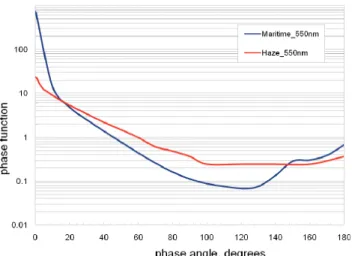
Fig. 2.Phase function of Arctic haze aerosol used in the simulation of aerosol effect on the spectral shape of snow surface. See text for details.
aerosol phase function for AOT values from 0 to 3. The aerosol phase function has been measured for 550 nm dur-ing the Arctic haze event on 23 March 2000, at Spitsbergen, Ny ˚Alesund, Svalbard, 78.923◦N, 11.923◦E, by the Alfred
Wegener Institute for Polar and Marine Research. It has a rather smooth shape without a significant increase of scat-tering in forward and backward directions (compared to rela-tively higher forward- and backscattering of maritime aerosol in Fig. 2), which is the feature of randomly shaped small ab-sorbing particles. This aerosol is composed predominantly of sulfate and sea salt, with lesser contributions from nitrate, soot, soil and trace elements, and organic compounds (Quinn et al., 2002). The typical background aerosol optical thick-ness for Arctic is around 0.05 (Tomasi et al., 2007). However, during Arctic haze events, the AOT can reach rather high val-ues of 0.5–1.0 and, therefore, can disturb the spectral shape of a scene.
5 5 0 660 870 1600 0 0.1 0.2 0.3 0.4 0.5 0.6 0.7 0.8 0.9 1 a
wa ve le ngth, nm
T O A re fl e c ta n c e 2 3 4 5 6 7 8 9 10 11
5 5 0 660 870 1600
0 0.1 0.2 0.3 0.4 0.5 0.6 0.7 0.8 0.9 1 b
wa ve le ng th, nm
T O A r e fl e c ta n c e
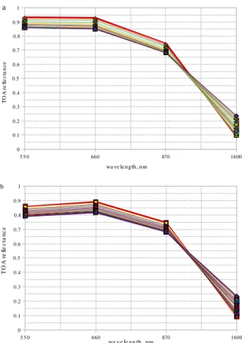
Fig. 3. The sensitivity of TOA reflectance over snow surface to aerosol load, simulated with RT calculations, for Lambertian snow
and aerosol only(a)and for snow, aerosol and O3absorption(b).
AOT changes from 0 to 3, with the step 0.2. AOT = 0 is shown with the thick red line. AOT = 3.0 is shown with the thick violet line.
observation geometries of AATSR – nadir view (viewing zenith angle is equal 0◦), rather low Sun (solar zenith angle
equal to 60◦), and the relative azimuth angle is equal to 0◦.
According to Mendonca et al. (1981), the single scattering albedo of Arctic haze appears to be rather high, larger than 0.9. Delene and Ogren (2002) reported the SSA of haze at Barrow, Alaska, to be 0.94. As we do not know the actual value of the SSA, we assume it to be 1 and compensate the possible lack of absorption with too high AOT. The aerosol is assumed to be uniformly distributed in a 3 km layer above the surface.
The result of such a simulation is the wavelength-dependence of TOA reflectance of the system “sur-face+atmosphere”. Here TOA reflectance is the amount of radiation, scattered at the surface and in the atmosphere (as seen from the top of the atmosphere), divided by the incident amount of radiation.
Figure 3a shows the result of our simulation for the dis-cussed surface and an aerosol load from 0 to 3.0 (step 0.2).
Fig. 4. The allowed amount of TOA reflectance scatter is shown for fresh dry snow (blue curve) and dry long grass (black curve). Violet and turquoise areas are the schematic view of the spectral shape criterion. They show where the corresponding spectral curve should go to still be recognized as snow. It is visible that dry long grass spectrum does not satisfy the spectral shape criterion, e.g. at channel 1.6 µm.
Figure 3b shows the same channels, surface and aerosols, but with included Rayleigh scattering and O3absorption.
It can be seen that the shape of the spectral curve does not depend on AOT for channels 550 nm, 660 nm, 870 nm in the “ideal” case (Fig. 3a) as well as in the “real” case with Rayleigh scattering and O3included. The inclusion of O3
absorption and Rayleigh scattering results in a slight decrease of TOA reflectance in the 550 nm channel.
As can also be seen from Fig. 3, over such a bright sur-face, the increasing of aerosol load in the atmosphere causes a darkening of the scene in channels 550 nm, 660 nm and 870 nm for the given geometry, due to scattering of light re-flected from the surface on aerosol layer and, thus, decreas-ing the upward flux at the TOA. Channel 1.6 µm reacts to an increase of AOT with an increase of the TOA reflectance, due to the fact that even a thin cloud of aerosol particles re-flects more than snow in this spectral region (snow albedo is around 0.1 here).
As a result, various aerosol loads (AOT from 0 to 3) affect TOA reflectance in 550 nm, 660 nm and 870 nm channels, causing an equal decrease in all these channels of about 10%. However, this does not affect the shape of the spectral curve. It is important to note that these effects are only valid for the discussed geometry and a very bright surface (Kokhanovsky et al., 2010).
Rayleigh scattering and O3absorption affect the shape of
1
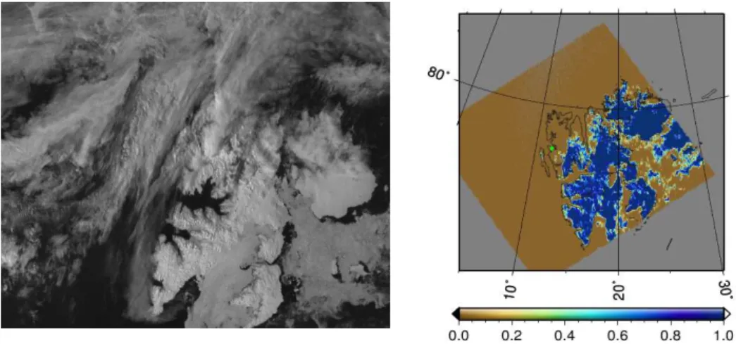
Fig. 5.The example of discussed cloud screening method:(a)the initial AATSR scene, 3 May 2006, Spitsbergen, 550 nm;(b)the probability of clear atmosphere over snow – the result of the cloud screening over snow routine.
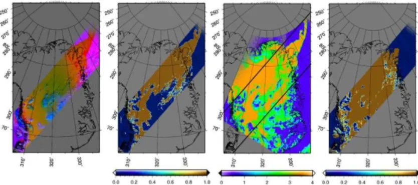
Fig. 6.Left panel shows the false colour composite (red is 11 µm BT, green is 550 nm reflectance, blue is 1.6 µm reflectance) of the initial AATSR scene, 11 May 2006, 16 h 26 min 26 s, orbit number 21938; middle panel is the screened AATSR scene, probability of clean snow; right panel is MODIS cloud mask: 1 – cloudy, 2 – probably cloudy, 3 – probably clear, 4 – clear. MODIS scene is for 11 May 2006, 16 h 40 min.
until AOT equals 3. All these factors disturb the shape of the snow spectrum and have to be taken into account during the analysis of the spectral behaviour of the scene reflectance.
The other factors which can disturb the shape of the spec-tral curve are caused by the physical parameters of snow and not by the atmosphere above it. They are snow grain size, liquid water content and possible impurities of the snowpack, which can be soot, dust, or atmospheric aerosols fallen out on the snow surface. All these factors have been studied and are presented in papers aimed at both modelling and measure-ments of snow optical properties.
The effect of dust and soot impurities in snow has been studied by Warren and Wiscombe (1980). It is shown that the VIS spectral region is particularly sensitive to these im-purities, whereas NIR and longwave emissivity of snow are not affected (which is important for Sect. 2.2). Of course, the distortion of snow albedo spectrum depends on the concen-tration of dust and soot. For example, 10 ppmw of soot can decrease the albedo of snow by more than 50% in VIS for an extremely large snow grain size of 1000 µm (Warren and Wiscombe, 1980). However, this effect is smaller for smaller grains and Arctic snow is believed to have a soot concentra-tion of around 0.2 ppmw, which reduces the snow albedo by approximately 20% in the 550 nm and 660 nm channels. For 870 nm, this effect is already less than 10%. Similar effects take place in case of dust impurities: depending on snow grain size, extremely high dust concentrations can reduce the VIS albedo of snow drastically, but dust concentrations of 10 ppmw decrease snow albedo by less than 10% in VIS, for both small and large grain sizes. Aoki et al. (2000) show the modelled spectral albedo of snow for several reasonable combinations of physical parameters such as snow density, impurities concentration, snow grain size and snow depth. These spectra differ from the pure snow spectrum only in the shortwave region and by no more than 10%, which proves that earlier discussed scatter values, caused by soot and dust, are sufficient for our task. The effect of snow age on the snow spectrum was studied by Domine et al. (2006). The comparison of wind crust, fresh snows and depth hoar spec-tra show that these specspec-tra are quite similar to each other in the visible, but differ more in the IR. The 1.6 µm channel reacts on the snow aging with a decreasing albedo, some-times almost to zero. However, this effect does not destroy the main feature of snow spectral signature – the spectacular drop of albedo from 0.87 µm to 1.6 µm. Liquid water con-tent, however, decreases the snow albedo also in the VIS and NIR (Gerland et al., 1999), but it does not change the spectral shape in the channels of AATSR and the relation between all the discussed VIS and NIR channels remains the same (War-ren, 1982).
The effect of snow grain size on the snow spectrum is studied, for example, by Domine et al. (2008), Wiscombe and Warren (1980) and Tedesco and Kokhanovsky (2007). The snow spectrum is affected by the grain size mostly in NIR and only a bit in VIS. Snow albedo in the 550 nm and
660 nm channels is affected only by a few percent, at 870 nm it goes up by around 10% for smaller grains and 10% down for larger grains. The snow albedo in the 1.6 µm channel in-creases for smaller grains up to 0.2 and drops down to almost zero for large grains, which is similar to the behaviour of the albedo in the 870 nm channel. This means that the relation between these two channels remains the same and the shape of the snow spectrum is not affected.
All the discussed disturbance factors (aerosol load, Rayleigh scattering, ozone, soot and dust impurities, age and liquid water content, and snow grain size) affect the spec-trum of the cloud free snow scene in different wavelength regions. The performed literature study and RT simulations made it possible to develop a criterion of snow spectral shape in VIS and NIR channels of AATSR. It is schematically shown in Fig. 4 for two example spectra. They are the fresh snow spectrum (from the ASTER spectral library, CalTech, 2008), represented with the blue curve and the dry long grass spectrum (from the USGC Spectroscopy Lab library), rep-resented with the black curve. Filled areas (violet for fresh snow and turquoise for dry long grass) show allowed free-dom in the shape of each spectrum. As the criterion is rela-tive, the allowed scatter will change from spectrum to spec-trum. We would like to underline that for our cloud screen-ing routine, we only need to analyse the shape of a spectrum in four VIS and NIR AATSR channels. These channels are shown in Fig. 4 by vertical lines. However, to make the con-cept more obvious, we extended the graphic representation of the shape criteria outside of the four discussed channels. The numerical criteria only exist for the four discussed chan-nels and should connect the TOA reflectances,RTOA(λ), of
those channels in the following way: RTOA(0.87 µm)−RTOA(1.6 µm)
RTOA(0.87 µm)
>80% (1)
RTOA(0.87 µm)−RTOA(0.66 µm) RTOA(0.87 µm)
<10% (2)
RTOA(0.66 µm)−RTOA(0.55 µm) RTOA(0.66 µm)
<40% (3)
Here the percentage is given for relative reflectance differ-ence with the relation toRTOA(870 nm) for the first two
cri-teria and toRTOA(660 nm) for the third one. From Fig. 4, it
is visible that the fresh snow spectrum (blue curve) fits into our snow spectral shape criteria, whereas the spectrum of dry long grass does not. TheRTOA(1.6 µm) of dry grass is too
high and does not represent the main feature of a snow spec-trum – the reflectance drop from 870 nm to 1.6 µm. Also, the feature of vegetation spectra, the so called “red edge” (fast increase of reflectance at 0.4–0.7 µm), is visible in the fig-ure and makes theRTOA(660 nm) be at the edge of the snow
The discussed criteria are already enough to screen out optically thick warm clouds, but will have difficulties with cirrus and any optically thin clouds, because these do not significantly disturb the spectral signature of snow in these spectral regions. To screen out such clouds, we need to use TIR channels of AATSR. This problem is discussed in the next section.
2.2 Cloud screening in TIR: snow emissivity and cloud reflectance
The 3.7, 10.8 and 12 µm channels provide additional infor-mation to distinguish surface and clouds. As was mentioned by Spangenberg et al. (2001), brightness temperature (BT) of the 3.7 µm channel contains not only emitted radiation, but also radiation scattered by the object, in our case, by a cloud or snow.
Thermal properties of snow have been measured (Hori et al., 2006; English et al., 1995) and show that snow is very close to a black body and emits according to its physical tem-perature. The reflection of snow is very low in the 3.7, 10.8 and 12 µm channels (Wald, 1994). This is not the case for clouds, because R(3.7 µm) of cloud droplets is much higher depending on the effective radii of the particles and on the optical thickness of the cloud. Therefore, the spectral shape of a cloud pixel in the discussed 3 channels will differ from that of snow due to the different physical nature of these two objects.
To estimate the amplitude of reflectance contamination of BT(3.7 µm), we calculate theRTOA(3.7 µm) according to
Spangenberg et al. (2001): RTOA(3.7 µm)=
ε3.7µm·B3.7µm(T3)−ε3.7µm·B3.7µm(T4)
µ0·S3.7µm−ε3.7µm·B3.7µm(T4) (4) whereT3is the measured 3.7 µm brightness temperature,T4
is the measured 11 µm brightness temperature,µ0is the
co-sine of solar zenith angle, S3.7µm is the solar constant at
3.7 µm (3.47 Wm−2µm−1)
,ε3.7µm is the clear snow
emit-tance, B3.7µm(BT) is the Planck function at 3.7 µm for some
temperature BT.
An example of a calculatedRTOA(3.7 µm) is presented in
Fig. 1e. One can clearly see the high reflectance of clouds and very low reflectance of snow and ocean (see ocean-land mask contours). This reflectance pattern is included in the AATSR BT(3.7 µm) (Fig. 1f), causing the differences in the shapes of the spectral curves of snow and clouds for 3.7, 10.8 and 12 µm channels. It is visible that the brightness tempera-ture of snow in all three channels is approximately the same, which corresponds to, e.g. measurements of snow emissivity in MODIS USCB Emissivity Library. Measured emissivity is quite stable throughout the thermal region of the spectrum (variation around 2%). Hori et al. (2006) show that emissiv-ity of snow for a given temperature depends on its physical parameters such as grain size and liquid water content. How-ever, these dependencies cause a variation of snow
emissiv-ity of less than 5%. This scatter of the spectral shape can be taken into account and is still much smaller than that caused by the high reflectance of clouds in the 3.7 µm channel.
Independently of the physical temperature of snow, the rel-ative BT differences of the 3.7, 10.8 and 12 µm channels are not to be larger than 3%. This criterion will remove both warm and cold clouds. Both are present in the discussed scene; in Fig. 1f, the blue colour corresponds to cold, and orange to warm clouds. BT of snow and ocean is similar in all three discussed channels within the allowed scatter.
All the factors mentioned in Sects. 2.1 and 2.2 create a spectral shape criterion for the relative reflectances and brightness temperatures in seven AATSR channels. It is not an absolute threshold in each of the channels separately, but rather a flexible relative connection of all the seven spectral channels in order to recognize the spectral signature of snow, if it is present in the spectrum of the scene.
To summarize, here are all the parts of the spectral shape criterion:
BT(3.7 µm)−BT(10.8 µm)
BT(3.7 µm)
<3% (5)
BT(3.7 µm)−BT(12 µm)
BT(3.7 µm)
<3% (6)
RTOA(0.87 µm)−RTOA(1.6 µm) RTOA(0.87 µm)
>80% (7)
RTOA(0.87 µm)−RTOA(0.66 µm) RTOA(0.87 µm)
<10% (8)
RTOA(0.66 µm)−RTOA(0.55 µm) RTOA(0.66 µm)
<40% (9)
Experiments show that this order of criteria is computation-ally the most effective, because most clouds are screened out during TIR check and the snow signature is mostly stored in the large drop between 870 nm and 1600 nm channels. None of these criteria are related to the absolute value of reflectance or BT; therefore, the algorithm does not rely on spatial contrast of the image in any channel.
The result of our cloud screening method is shown in Fig. 5 (unscreened scene in all the 7 AATSR channels is shown in Fig. 1).
3 Validation of the algorithm
3.1 MPL
Fig. 8. Alaska, AATSR: 30 April 2006, 22 h 17 min 44 s, orbit number 21783. MODIS: 30 April 2006, 22 h 5 min. Left panel is the false colour composite (red is 11 µm BT, green is 550 nm reflectance, blue is 1.6 µm reflectance) of initial AATSR scene; second left panel is the clear snow mask of AATSR scene (0 – not snow, 1 – clear snow) achieved with presented method; third left panel is MODIS cloud mask: 1 – cloudy, 2 – probably cloudy, 3 – probably clear, 4 – clear; right panel is operational AATSR cloud mask from level-1b product: 0 – cloudy, 1 – clear.
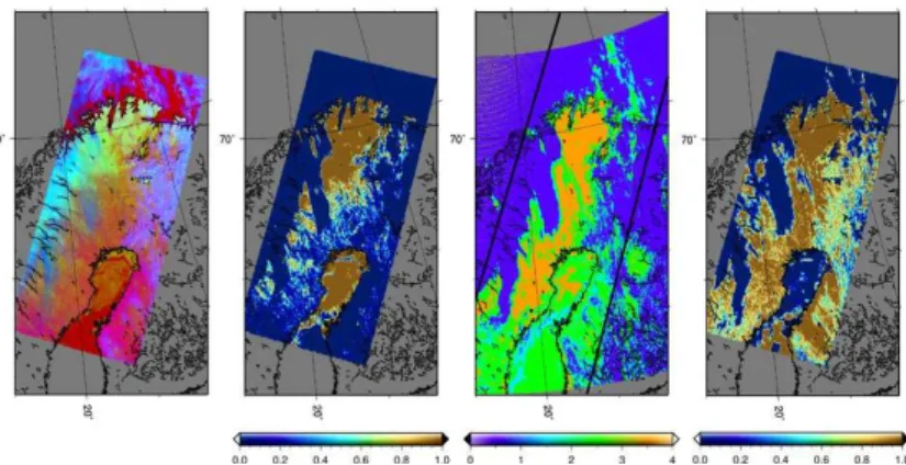
Fig. 9. Greenland. AATSR: 4 May 2005, 15 h 7 min 47 s, orbit number 21836, MODIS: 4 May 2005, 15 h 0 min. Left panel is the false colour composite (red is 11 µm BT, green is 550 nm reflectance, blue is 1.6 µm reflectance) of initial AATSR scene; second left panel is the clear snow mask of AATSR scene (0 – not snow, 1 – clear snow) achieved with presented method; third left panel is MODIS cloud mask: 1 – cloudy, 2 – probably cloudy, 3 – probably clear, 4 – clear; right panel is operational AATSR cloud mask from level-1b product: 0 – cloudy, 1 – clear.
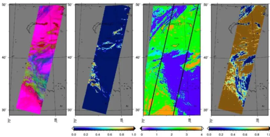
Fig. 11. Scandinavian Peninsula, AATSR: 22 April 2006, 9 h 47 min 27 s, orbit number 21661. MODIS: 22 April 2006, 9 h 40 min. Left panel is the false colour composite (red is 11 µm BT, green is 550 nm reflectance, blue is 1.6 µm reflectance) of initial AATSR scene; second left panel is the clear snow mask of AATSR scene (0 – not snow, 1 – clear snow) achieved with presented method; third left panel is MODIS cloud mask: 1 – cloudy, 2 – probably cloudy, 3 – probably clear, 4 – clear; right panel is operational AATSR cloud mask from level-1b product: 0 – cloudy, 1 – clear.
Fig. 12. Northern part of Russia. AATSR: 22 April 2006, 4 h 43 min 20 s, orbit number 21658. MODIS: 22 April 2006, 4 h 45 min. Left panel is the false colour composite (red is 11 µm BT, green is 550 nm reflectance, blue is 1.6 µm reflectance) of initial AATSR scene; second left panel is the clear snow mask of AATSR scene (0 – not snow, 1 – clear snow) achieved with presented method; third left panel is MODIS cloud mask: 1 – cloudy, 2 – probably cloudy, 3 – probably clear, 4 – clear; right panel is operational AATSR cloud mask from level-1b product: 0 – cloudy, 1- clear.
Fig. 14.Himalayan mountains. AATSR: 18 April 2006, 5 h 17 min 59 s, orbit number 21601. MODIS: 18 April 2006, 5 h 20 min. Left panel is the false colour composite (red is 11 µm BT, green is 550 nm reflectance, blue is 1.6 µm reflectance) of initial AATSR scene; second left panel is the clear snow mask of AATSR scene (0 – not snow, 1 – clear snow) achieved with presented method; third left panel is MODIS cloud mask: 1 – cloudy, 2 – probably cloudy, 3 – probably clear, 4 – clear; right panel is operational AATSR cloud mask from level-1b product: 0 – cloudy, 1 – clear.
wrong detections are connected to thin clouds (Fig. 6), which disturb the spectral shape of the scene only slightly, or to a particular case of surface (Fig. 7).
In Fig. 6, we see the scene for Spitsbergen, 11 May 2006. Micro Pulse Lidar located in Ny ˚Alesund (78◦.91667 N,
11◦.93300 E), in the western part of the island. It shows the
presence of a very thin cloud at a 1 km altitude, however, neither discussed cloud-screening technique nor the MODIS cloud mask show it. At the same time, their correspondence to each other is rather good throughout the rest of the im-age. The reason can be the size of the cloud: subpixel thin clouds over snow simply do not change the spectral shape of the scene significantly.
In Fig. 7, we see another scene for Spitsbergen, 8 May 2006. According to Micro Pulse Lidar, the Ny ˚Alesund area should be cloud free. However, our cloud screening shows that there is no clear snow at Ny ˚Alesund on this scene. The MODIS cloud product shows this area as “probably clear”. AATSR reflectance shows that the surface is slightly darker at Ny ˚Alesund. This can be caused by shadowing by moun-tains or extremely contaminated snow surface.
So we see that thin clouds are, unfortunately, still a prob-lem for the discussed cloud screening method. Of course, one could give more strict spectral shape criteria and reduce the allowed scatter. However, this could lead to screening out of pixels with the present aerosol loads or pixels with those various kinds of snow which differ from the fresh clean snow. In other words, the spectral shape criterion can be ad-justed to fit the certain task. If the task is to study physical properties of snow (where atmospheric correction is usually a problem), one could set the allowed scatter to be very nar-row along the desired spectrum. Such a criterion would only give the scenes with clean fresh snow, according to the ref-erence spectrum (see e.g. Fig. 4). The influence of the
at-mosphere here will be very small and all the exotic types of snow will also be absent. On the other hand, if the objective is to study atmosphere and, for example, to retrieve AOT over snow, then the allowed range of scatter should be rather wide, to ensure that high aerosol loads are not screened. However, a broad criterion for scatter yields scenes with various types of snow, possibly contaminated. Thus, the target product for the retrieval (in this case AOT over snow retrieval) needs to be considered.
3.2 The comparison to MODIS and operational AATSR cloud masks for different kinds of snow surface
In order to check the performance of the presented cloud screening method over different kinds of snow surface, we processed a set of AATSR scenes from both Northern and Southern hemispheres at various locations, and compared the results of operational AATSR cloud mask for nadir view, which is taken from a level 1b AATSR product, and to the MODIS cloud product for the same location. Unfortu-nately, exact temporal collocation of AATSR and MODIS was sometimes impossible, in which case the closest avail-able observation was chosen. Pixel-to-pixel collocation of the two instruments appear to be not easy, but visual analy-sis can already help to estimate the quality of the presented method. It is important to note that MODIS and operational AATSR cloud masks detect cloudy or clear conditions over any kind of surface, whereas the presented method has been designed to detect clear snow scenes only. Therefore, as dis-cussed, the snow mask will differ from operational AATSR and MODIS cloud masks even in cloud-free cases – due to the presence of all kinds of surface in these latter products and not just snow.
operational cloud mask for eight different cases of clouds over snow are shown in Figs. 8–15. They include scenes over Alaska (snow, ice covered with snow), Greenland (snow, ice covered with snow), the Scandinavian Peninsula (snow cov-ered mountains, snow covcov-ered forest), Northern part of Rus-sia (snow covered forest, snow on ice), Himalayan mountains (snow covered peaks), Antarctica (snow, snow covered ice).
Figures 8–13 show that the presented cloud-screening method corresponds to MODIS cloud mask rather well, screening out all the clouds and not confusing them with snow (Fig. 10). Flat snow, either on ice or on land, is the best surface for the cloud screening (Figs. 8–9, ice part of Fig. 12). Mountain peaks covered with snow can be recog-nized (Figs. 10, 11, 14). Snow covered forest (Fig. 11) is also recognized (however, not continuously; only single brightest snow pixels are detected). In general, the presented method appears to be a little stricter in comparison to the MODIS cloud mask. For example, the case of flat snow, according to the MODIS cloud product, is not recognized very well (Fig. 15, Antarctica). The reason for a not very accurate de-tection might be the illumination-observation geometry (low solar zenith angle), which could affect the ranges of appli-cability of the presented spectral shape criteria. Addition-ally, the reason might be some type of snow here overlooked, which is located outside the suggested spectral shape crite-rion, but still is a cloud-free and not extremely contaminated snow. Extensive research is needed to understand if this is the feature of all the Antarctic snow or just the feature of one special day or location.
AATSR operational cloud mask corresponds to MODIS and presented snow mask rather well in some cases (Figs. 10, 11, lower part of Fig. 12), however, showing not so good a performance for other cases of snow surfaces, where pre-sented snow mask and MODIS cloud mask still correspond well (Figs. 8, 9 12, 13). Therefore, for the cases of snow sur-face, the reliability of AATSR operational cloud mask should be investigated further.
In general, according to the comparison to MODIS cloud mask, the quality of the presented cloud/snow discrimination appears to be reasonably good for such a simple discrimina-tion algorithm.
4 Conclusions
A simple and robust cloud-screening method was developed for AOT retrieval over snow using AATSR observations. The method uses a spectrum-shape control in seven VIS, NIR and TIR AATSR channels and does not require time-sequences of data, morphological analysis of the scene or manual tun-ing to set absolute thresholds. The method was compared to MODIS cloud mask for various dates and locations and showed good correspondence with it over flat snow, covered mountain peaks, covered forest and snow-covered ice. Both MODIS cloud mask and presented snow
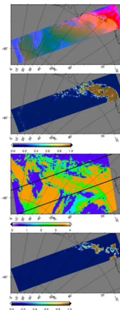
Fig. 15. Antarctica, AATSR: 20 January 2006, 5 h 16 min 00 s, or-bit number 20341. MODIS: 20 January 2006, 5 h 00 min. Top panel is the false colour composite (red is 11 µm BT, green is 550 nm re-flectance, blue is 1.6 µm reflectance) of initial AATSR scene; sec-ond from top panel is the clear snow mask of AATSR scene (0 – not snow, 1 – clear snow) achieved with presented method; third from top panel is MODIS cloud mask: 1 – cloudy, 2 – probably cloudy, 3 – probably clear, 4 – clear; lowest panel is operational AATSR cloud mask from level-1b product: 0 – cloudy, 1 – clear.
Edited by: J. Joiner
References
Ackerman, S. A., Strabala, K. I., Menzel, W. P., Frey, R. A., Moeller, C. C., and Gumley, L. E.: Discriminating clear sky from clouds with MODIS, J. Geophys. Res., 103, 32141–32157, 1998. Allen, R. C., Durkee, P. A., and Wash, C. H.: Snow/cloud discrim-ination with multispectral satellite measurements, J. Appl. Me-teor., 29, 994–1004, 1990.
Aoki, Te., Aoki, Ta., Fukabori, M., Hachikubo, A., Tachibana, Y., and Nishio, F.: Effects of snow physical parameters on spectral albedo and bidirectional reflectance of snow surface, J. Geophys. Res, 105, D8, 10219–10236, doi:10.1029/1999JD901122, 2000. Br´eon, F.-M. and Colzy, S.: Cloud detection from the spaceborne POLDER instrument and validation against surface synoptic ob-servations, J. Appl. Meteor., 38, 777–785, 1999.
Campbell, J. R., Hlavka, D. L., Welton, E. J., Flynn, C. J., Turner, D. D., Spinhirne, J. D., Scott, V. S., and Hwang, I. H.: Full-Time, Eye-Safe Cloud and Aerosol Lidar Observation at Atmo-spheric Radiation Measurement Program Sites: Instruments and Data Processing, J. Atmos. Oceanic Tech., 19, 431–442, 2002. Delene, D. J. and Ogren, J. A.: Variability of aerosol optical
prop-erties at four North American surface monitoring sites, J. Atmos. Sci., 59, 1135–1150, 2002.
Diner, D., Clothiaux, E., and Di Girolamo, L.: MISR Multi-angle imaging spectro-radiometer algorithm theoretical basis. Level 1 Cloud detection, Jet Propulsion Laboratory, JPL D-13397, 1999.
Domine, F., Albert, M., Huthwelker, T., Jacobi, H.-W.,
Kokhanovsky, A. A., Lehning, M., Picard, G., and Simpson, W. R.: Snow physics as relevant to snow photochemistry, Atmos. Chem. Phys., 8, 171–208, doi:10.5194/acp-8-171-2008, 2008. Domine, F., Salvatori, R., Legagneux, L., Salzano, R., Fily, M., and
Casacchia, R.: Correlation between the specific surface area and the short wave infrared (SWIR) reflectance of snow, Cold Reg. Sci. Technol., 46, 60–68, 2006.
English, S. J., Jones, D. C., Hewison, T. J., Saunders, R. W., and Hallikainen, M.: Observations of the emissivity of snow and ice surfaces from the SAAMEX and MACSI airborne campaigns, Geoscience and Remote Sensing Symposium, 1995. IGARSS ’95, “Quantitative Remote sensing for Science and Applica-tions”, International, vol. 2, 1493–1495, 1995.
Gafurov, A. and B´ardossy, A.: Cloud removal methodology from MODIS snow cover product, Hydrol. Earth Syst. Sci., 13, 1361– 1373, doi:10.5194/hess-13-1361-2009, 2009.
Gerland, S., Winther, J.-G., Ørbæk, J. B., Liston, G. E., Øritsland, N. A., Blanco, A., and Ivanov, B.: Physical and optical properties of snow covering Arctic tundra on Svalbard, Hydrol. Process., 13, 2331–2343, 1999.
Hori, M., Aoki, Te., Tanikawa, T., Motoyoshi, H., Hachikubo, A., Sugiura, K., Yasunari, T. J., Eide, H., Storvold, R., Nakajima, Y., and Tand akahashi, F.: In-situ measured spectral directional emissivity of snow and ice in the 8–14 um atmospheric window, Remote Sens. Environ., 100, 486–502, 2006.
Istomina, L. G., von Hoyningen-Huene, W., Kokhanovsky, A. A., and Burrows, J. P.: Retrieval of aerosol optical thickness in Arc-tic region using dual-view AATSR observations, Proc. ESA
At-mospheric Science Conference, Barcelona, Spain, 7–11 Septem-ber 2009, ESA SP-676, 2010.
Istomina, L. G., von Hoyningen-Huene, W., Kokhanovsky, A. A., Rozanov, V. V., Schreier, M., Dethloff, K., Stock, M., Treffeisen, R., Herber, A., and Burrows, J. P.: Sensitivity study of the dual-view algorithm for aerosol optical thickness retrieval over snow and ice, Proc. 2nd MERIS/(A)ATSR user workshop, ESRIN, Frascati, Italy, 22–26 September 2008, ESA SP-666, 2009. Key, J. and Barry, R. G.: Cloud cover analysis with Arctic AVHRR
data. 1. Cloud detection, J. Geophys. Res., 94, D15, 18521– 18535, 1989.
Kokhanovsky, A. A.: Cloud Optics, Eds.: Mysak, L. A., Hamilton, K., Publ. Springer, 2006.
Kokhanovsky, A. A, Rozanov, V. V., Aoki, T., Odermatt, D., Brock-mann, B., Kr¨uger, O., Bouvet, M., Drusch, M., and Hori, M.: Sizing of snow grains using backscattered solar light, Int. J. Re-mote Sens., in press, 2010.
Krijger, J. M., Aben, I., and Schrijver, H.: Distinction
be-tween clouds and ice/snow covered surfaces in the identifica-tion of cloud-free observaidentifica-tions using SCIAMACHY PMDs, At-mos. Chem. Phys., 5, 2729–2738, doi:10.5194/acp-5-2729-2005, 2005.
Liu, Y., Key, J. R., Frey, R. A., Ackerman, S. A., and Menzel, W. P.: Nighttime polar cloud detection with MODIS, Remote Sens. Environ., 92, 181–194, 2004.
Lotz, W. A., Vountas, M., Dinter, T., and Burrows, J. P.: Cloud and surface classification using SCIAMACHY polariza-tion measurement devices, Atmos. Chem. Phys., 9, 1279—1288, doi:10.5194/acp-9-1279-2009, 2009.
Lyapustin, A., Tedesco, M., Wang, Y., Aoki, T., Hori, M., and Kokhanovsky, A.: Retrieval of snow grain size over Greenland from MODIS, Remote Sens. Environ., 113, 1976–1987, 2009. Lyapustin, A. and Wang, Y.: The time series technique for aerosol
retrievals over land from MODIS, in: Satellite Aerosol Remote Sensing over Land, edited by: Kokhanovsky A. A., de Leeuw, G., Springer Praxis Publ. Chichester, 69–99, 2009.
Lyapustin, A., Wang, Y., and Frey, R.: An automated cloud mask algorithm based on time series of MODIS measurements, J. Geo-phys. Res., 113, D16207, doi:10.1029/2007JD009641, 2008. Martins, J. V., Tanr´e, D., Remer, L., Kaufman, Y., Mattoo, S.,
and Levy, R.: MODIS Cloud screening for remote sensing of aerosols over oceans using spatial variability, Geophys. Res. Lett., 29(12), 8009, doi:10.1029/2001GL013252, 2002. Mendonca, B. G., DeLuisi, J. J., and Schroeder, J. A.: Arctic Haze
and perturbation in the solar radiation fluxes at Barrow, Alaska, Proceedings from the 4th Conference on Atmospheric Radiation, Atm. Met. Sco., Toronto, Ontario, Canada, 95–96, 1981. Minnis, P., Chakrapani, V., Doelling, D. R., Nguyen, L., Palikonda,
R., Spangenberg, D. A., Uttal, T., Arduini, R. F., and Shupe, M.: Cloud coverage and height during FIRE ACE derived from AVHRR data, J. Geophys. Res., 106, D14, 15215–15232, 2001. Quinn, P. K., Miller, T. L., Bates, T. S., Ogren, J. A., Andrews, E.,
and Shaw, G. E. : A three-year record of simultaneously mea-sured aerosol chemical and optical properties at Barrow, Alaska, J. Geophys. Res., 107, D11, 15pp., doi:10.1029/2001JD001248, 2002.
range, Adv. Space Res., 36, 1015–1019, 2005.
Spangenberg, D. A., Chakrapani, V., Doelling, D. R., Minnis, P., and Arduini, R. F.: Development of an automated Arctic cloud mask using clear-sky satellite observations taken over the SHEBA and ARM NSA sites, Proc. 6th Conf. on Polar Meteor. and Oceanography, San Diego, CA, 14–18 May 2001, 246–249, 2001.
Tedesco, M. and Kokhanovsky, A. A.: The semi-analytical snow retrieval algorithm and its application to MODIS data, Remote Sens. Environ., 110, 317–331, 2007.
Tomasi, C., Vitale, V., Lupi, A., Di Carmine, C., Campanelli, M., Herber, A., Treffeisen, R., Stone, R. S., Andrews, E., Sharma, S., Radionov, V., von Hoyningen-Huene, W., Stebel, K., Hansen, G. H., Myhre, C. L., Wehrli, C., Aaltonen, V., Lihavainen, H., Virkkula, A., Hillamo, R., Str¨om, J., Toledano, C., Ca-chorro, V. E., Ortiz, P., de Frutos, A. M., Blindheim, S., Frioud, M., Gausa, M., Zielinski, T., Petelski, T., and Yamanouchi, T.: Aerosols in polar regions: A historical overview based on optical depth and in situ observations, J. Geophys. Res., 112, D16205, doi:10.1029/2007JD008432, 2007.
Trepte, Q., Arduini, R. F., Chen, Y., Sun-Mack, S., Minnis, P., Spangenberg, D. A., and Doelling, D. R.: Development of a day-time polar cloud mask using theoretical models of near-infrared bidirectional reflectance for ARM and CERES, Proc. AMS 6th Conf. Polar Meteorology and Oceanography, San Diego, CA, 4– 18 May , 242–245, 2001.
Wald, A. E.: Modeling thermal infrared (2–14 µm) reflectance spec-tra of frost and snow, J. Geophys. Res., 99, B12, 24241–24250, 94JB01560, 1994.
Warren, S. G.: Optical Properties of Snow, Rev. Geophys., 20(1), 67–89, 1982.
Warren, S. G. and Wiscombe, W. J.: A model for the spectral albedo of snow. II: Snow containing atmospheric aerosols, J. Atmos. Sci. 37, 2734–2733, 1980.
Welton, E. J., Campbell, J. R., Spinhirne, J. D., and Scott, V. S.: Global monitoring of clouds and aerosols using a network of micro-pulse lidar systems, Proc. Int. Opt. Eng. 4153, 151–158, 2001.