www.atmos-chem-phys.net/11/293/2011/ doi:10.5194/acp-11-293-2011
© Author(s) 2011. CC Attribution 3.0 License.
Chemistry
and Physics
Modeling natural emissions in the Community Multiscale Air
Quality (CMAQ) model – Part 2: Modifications for simulating
natural emissions
S. F. Mueller, Q. Mao, and J. W. Mallard
Tennessee Valley Authority, P.O. Box 1010, Muscle Shoals, Alabama 35662-1010, USA Received: 28 May 2010 – Published in Atmos. Chem. Phys. Discuss.: 28 June 2010 Revised: 10 December 2010 – Accepted: 17 December 2010 – Published: 14 January 2011
Abstract. The Community Multiscale Air Quality (CMAQ) model version 4.6 has been revised with regard to the repre-sentation of chlorine (HCl, ClNO2) and sulfur (dimethylsul-fide, or DMS, and H2S), and evaluated against observations and earlier published models. Chemistry parameterizations were based on published reaction kinetic data and a recently developed cloud chemistry model that includes heteroge-neous reactions of organic sulfur compounds. Evaluation of the revised model was conducted using a recently enhanced data base of natural emissions that includes ocean and con-tinental sources of DMS, H2S, chlorinated gases and light-ning NOx for the continental United States and surround-ing regions. Results ussurround-ing 2002 meteorology and emissions indicated that most simulated “natural” (plus background) chemical and aerosol species exhibit the expected seasonal variations at the surface. Ozone exhibits a winter and early spring maximum consistent with ozone data and an earlier published model. Ozone distributions reflect the influences of atmospheric dynamics and pollutant background levels imposed on the CMAQ simulation by boundary conditions derived from a global model. A series of model experi-ments reveals that the consideration of gas-phase organic sul-fur chemistry leads to sulfate aerosol increases over most of the continental United States. Cloud chemistry parameteriza-tion changes result in widespread decreases in SO2across the modeling domain and both increases and decreases in sulfate. Most cloud-mediated sulfate increases occurred mainly over the Pacific Ocean (up to about 0.1 µg m−3) but also over and downwind from the Gulf of Mexico (including parts of the eastern US). Geographic variations in simulated SO2and sul-fate are due to the link between DMS/H2S and their byprod-uct SO2, the heterogeneity of cloud cover and precipitation
Correspondence to:S. F. Mueller ([email protected])
(precipitating clouds act as net sinks for SO2 and sulfate), and the persistence of cloud cover (the largest relative sul-fate increases occurred over the persistently cloudy Gulf of Mexico and western Atlantic Ocean). Overall, the addition of organic sulfur chemistry increased hourly surface sulfate levels by up to 1–2 µg m−3but reduced sulfate levels in the vicinity of high SO2 emissions (e.g., wildfires). Simulated surface levels of DMS compare reasonably well with obser-vations in the marine boundary layer where DMS oxidation product levels are lower than observed. This implies either a low bias in model oxidation rates of organic sulfur species or a low bias in the boundary conditions for DMS oxidation products. This revised version of CMAQ provides a tool for realistically simulating the influence of natural emissions on air quality.
1 Introduction
The Community Multiscale Air Quality (CMAQ) Model, developed by the US Environmental Protection Agency (EPA), is typically used to examine the formation and trans-port of ozone and airborne particles. The EPA Models-3 air quality modeling system – including the SMOKE emissions and CMAQ air quality components – simulates pollutants emitted from both anthropogenic and natural processes and systems. Common natural pollutants in SMOKE/CMAQ are biogenic emissions of volatile organic compounds (VOCs) emitted by vegetation, soil NO emissions, gaseous and par-ticulate emissions from wildfires, and animal-derived NH3. Recently, windblown dust emissions were added using the model of Mansell et al. (2006). In addition, beginning with version 4.6 (denoted “CMAQ4.6”), CMAQ performs an in-ternal computation of sea salt particle emissions. These nat-ural emission treatments in the SMOKE/CMAQ4.6 system are incomplete, however.
Berntsen and Isaksen (1997) modeled global tropospheric photochemistry based on the Global Emissions Inventory Activity (GEIA) emissions data base (http://www.geiacenter. org/). This data base includes both anthropogenic and natural emissions, the latter including fluxes from biomass burning, biogenic sources (vegetation VOCs and soil NO), lightning NOx(LNOx)and oceans [dimethylsulfide (DMS), NH3, HCl and ClNO2]. However, given the focus of Berntsen and Isak-sen (1997) on ozone it is not clear to what extent their model-ing used all the emissions species that are currently available. Park et al. (2004) used GEOS-Chem to simulate atmo-spheric aerosols derived in part from natural sulfur emis-sions from oceans (DMS) and volcanoes; NOx from light-ning, vegetation, and soils; biomass burning emissions (in-cluding CO, NOxand VOCs); and ammonia emitted by an-imals. Likewise, Kaminski et al. (2008) used data from the EDGAR 2.0 and GEIA emissions inventories for their global air quality modeling effort including emissions from these same sources. They incorporated monthly mean totals of LNOx from the GEIA data base, scaling emission hori-zontally according to the modeled distribution of convective clouds and vertically following profiles reported by Picker-ing et al. (1993).
Koo et al. (2010) recently examined potential air quality impacts of selected natural emissions not normally treated in the CMAQ Model. They added lightning NOxand surrogates for organosulfur from oceans. Their approach to estimat-ing LNOxemissions started with an annual estimate to total LNOxemitted across the United States followed by a spatial-temporal allocation scheme based on simulated convective precipitation. Organosulfur species DMS and methanesul-fonic acid (MSA) were treated using ocean emissions es-timates from the global GEOS-Chem model, and by using SO2 as a surrogate for DMS and sulfate as a surrogate for MSA. This approach avoided the need for modifying the model chemistry but poses questions about the validity of their assumptions. Koo et al. (2010) concluded that LNOx contributes significantly (1–6 ppbV) to annual average ozone
levels, especially across the southeastern US. They also de-termined that their scheme for estimating organosulfur pollu-tants decreased ozone slightly (due to the added sulfur react-ing with OH) in the vicinity of the emissions and increased fine particle mass by amounts generally<0.25 µg m−3on an annual average.
Reduced sulfur (DMS and H2S) emissions from oceans and geogenic sources, overlooked in CMAQ, are considered an important source of marine aerosols (Kreidenweis et al., 1991). Though relatively small compared to the oceans, in-land lakes and coastal wetin-lands are also important sources of DMS and H2S (NAPAP, 1991). Geogenic sources – es-pecially the thermal vents of geologically active regions like Yellowstone National Park – emit H2S that may be important contributors to downwind aerosols. Emissions from volca-noes were generally not included due to the sporadic nature of their emissions.
Gas-phase Chemistry: Kreidenweis et al. (1991) used a photochemical model with 72 chemical reactions (and 12 photolysis reactions) to examine sulfate aerosol formation in the marine environment. However, their model contained only one reaction involving DMS oxidation by OH with SO2 and MSA as products. This highly simplified approach was sufficient to produce a latitudinal gradient in marine sulfate similar to that reported from some measurement studies. No reactions were included that treated H2S.
Yin et al. (1990) developed a comprehensive model of DMS and its derivatives. Their mechanism included 40 sul-fur species and 140 reactions. Zaveri (1997) simplified the Yin et al. mechanism (10 organic sulfur species and 30 reac-tions) for use in a large-scale atmospheric model. The Zaveri model retained the major oxidation pathways from its more complex progenitor, but several reactions were combined and/or simplified to reduce computational requirements. Za-veri’s work focused most attention on the fate of two radi-cals formed as part of the DMS-to-sulfate channels: CH3SO2 and CH3SO3. The reason for this is that CH3SO2is formed as part of several reaction channels (while CH3SO3is pro-duced from some reactions involving CH3SO2)but its fate has been less certain than other intermediate species. The uncertainty is due to the relative importance of the thermal decomposition of CH3SO2to CH3and SO2, versus reactions of CH3SO2with species such as NO2, O3and HO2. Prior to Zaveri’s work, different laboratory studies of this decom-position yielded rates that differed by a factor of 3×10⁵. Clearly, this uncertainty – plus the uncertainty of the rate constants for chemical reactions involving CH3SO2– made it difficult to know whether these reactions were of sufficient significance to include in a mechanism for marine sulfate. Zaveri concluded that the competing reactions were impor-tant and included them (plus reactions involving CH3SO3) in his mechanism.
although differences exist in the rate constants and branching or partitioning ratios for some of the reactions. DMS is ini-tially attacked by OH with two reaction channels (all mech-anisms), NO3(all mechanisms) and O (Yin et al. and Zaveri mechanisms). One DMS + OH channel produces dimethyl-sulfoxide (DMSO), dimethylsulfone (DMSO2), methane-sulfinic acid (MSIA) and MSA (only the Lucas and Prinn mechanism includes DMSO2). The other OH channel leads to the formation of the hydroperoxy radical CH3SCH2OO which undergoes further reactions that produce CH3S and, ultimately, SO2 and H2SO4 (all but the Lucas and Prinn mechanism). Only the Yin et al. and Zaveri mechanisms in-clude reactions for CH3SO2and CH3SO3.
A study by Kukui et al. (2000) – published after Yin et al. (1990) and Zaveri (1997), and too late to be included in the overview of Finlayson-Pitts and Pitts (2000) – examined in detail the issue of CH3SO2thermal decomposition. Kukui et al. (2000) measured CH3SO2behavior and their data, cou-pled with theory, were used to develop a mathematical ex-pression for CH3SO2 thermal decomposition as a function of temperature and pressure. This expression represents the CH3SO2loss rate throughout the troposphere for comparison with CH3SO2 loss rates for its reactions with NO2, O3 and HO2 at realistic concentrations based on the rate constants used by Zaveri (1997). The pressure/temperature effect on thermal decomposition was examined for a range of condi-tions that can occur between the ground and the top of the troposphere. Colder temperatures in the upper troposphere significantly reduce CH3SO2decomposition. However, the loss rate due to decomposition in the troposphere is almost always at least a factor of ten greater than loss rates from reactions with NO2, O3 and HO2. Based on this, it seems that including reactions involving CH3SO2 and CH3SO3 in a chemical mechanism is likely a computational luxury that many models cannot afford.
Chlorine Compounds: over the oceans halogens, espe-cially chlorine, comprise an important source of reactive compounds (Smith and Mueller, 2010). In this environment away from continental pollutants, emissions of reduced sul-fur species such as DMS and H2S react primarily with OH in the atmosphere but their oxidation is accelerated in the presence of HCl and ClNO2. Chlorine reactants originate from the nighttime heterogeneous reaction of N2O5with sea salt aerosols – releasing ClNO2(Behnke et al., 1997) – and from other reactions involving sea salt aerosols and produc-ing chlorine gas and HCl (Knippproduc-ing and Dabdub, 2003). Chlorine gas photolyzes in the atmosphere to atomic chlorine and ClNO2reacts with OH to form HOCl and NO2 (Atkin-son et al., 2007):
OH+ClNO2→HOCl+NO2 (R1)
Thus, ClNO2is a reservoir of NO2in the marine boundary layer and provides reactive HOCl that further photolyzes in the gas phase to OH and Cl. Nitryl chloride is produced at levels roughly 100 times lower than HCl (Erickson et al.,
1999). Ambient concentrations of Cl are generally low ex-cept in areas affected by anthropogenic chlorine and/or NOx emissions. Table 1 lists Reaction (R1) along with several reactions believed by Tanaka and Allen (2001) to be impor-tant in tropospheric chemistry for chlorine species. Note that HCl can be an important contributor to cloud droplet acidity in the marine environment and aqueous Cl−plays a role in the droplet balance of various chlorine species in clouds.
H2S: atmospheric oxidation of H2S proceeds follow-ing a variety of gas-phase reactions involvfollow-ing many of the same species important for other photochemistry. Ki-netic data exist for reactions of H2S with OH, O, HO2, Cl and NO3. Each of the OH, O and Cl radicals is known to attack the S bond with H and produce the SH radi-cal. Both HO2 and NO3 are likely to act similarly on H2S although their reaction products have not been directly identified. The rate constant for H2S+Cl has been mea-sured to be the highest (7.4×10⁻¹¹cm3molecule−1s−1 at 298 K) of this set of reactions. The next highest rate con-stants are for reactions involving OH and O (at 298 K): k≈5×10⁻¹²cm3molecule−1s−1 for the OH reaction is about two orders of magnitude greater than that for the O reaction (NASA, 1997). Upper limits to the rate constants for the reactions involving HO2 and NO3 are both ∼1×
10−15cm3molecule−1s−1 (Atkinson et al., 2004). During daytime, the reaction of H2S with OH will dominate over that with O, while the reaction with Cl could be important over the ocean and in the presence of chlorine emissions. At night, the reaction with NO3will most likely be the domi-nant pathway for initiating the breakdown of H2S with as-sumed products (by analogy with the other reactions) of SH and nitric acid. Table 2 summarizes noteworthy H2S and re-lated reactions along with relevant kinetic data and literature citations.
SH Reactions: the second step in oxidizing H2S in the atmosphere involves reactions of SH. Data exist on the ki-netics of SH reactions with O, O2, O3, NO, NO2, Cl2 and H2O2, as well as various bromine and fluorine species (NASA, 1997). At 298 K, rate constants ki for SH
re-actions with species i are as follows (all have units of cm3molecule−1s−1): kO=1.6×10⁻¹⁰; kO2<4×10
−19; kO3=3.7×10⁻¹²;kNO2=6.5×10⁻¹¹;kCl2=1.7×10⁻¹⁰; kH2O2 <5×10
−15. The reaction SH + NO + M has a more complex rate constant expression that is a function of alti-tude (pressure) in the atmosphere. At sea level and 298 K kN O=2.6×10⁻¹²cm3molecule−1s−1. The slowest
Table 1.Chlorine reactions with importance to tropospheric gas-phase chemistrya.
Reactionb Rate Constantc,k
(cm3molecule−1s−1)
Cl2+hν→2 Cl 0.264kNO2
HOCl +hν→OH+Cl 0.51kACRO
PAR+Cl→HCl+0.87 XO2+0.13 XO2N+0.11 HO2+0.11 ALD2 +0.76 ROR−0.11 PAR 78kOH+PAR OLE+Cl→FMCL+ALD2+2 XO2+HO2−PAR 20kOH+OLE
CH4+Cl→HCl+XO2+HCHO+HO2 6.6×10⁻¹²exp(−1240/T) ETH+Cl→2 XO2+HCHO+FMCL+HO2 12.6kOH+ETH
ISOP+Cl→0.15 HCl+XO2+HO2+0.28 ICL1 4.5kOH+ISOP
ICL1+OH→ICL2 0.19kOH+ISOP
Cl+O3→ClO+O2 2.9×10⁻¹¹exp(−260/T) ClO+NO→Cl+NO2 6.2×10⁻¹²exp(295/T) ClO+HO2→HOCl+O2 4.6×10⁻¹³exp(710/T) ClNO2+OH→HOCl+NO2 2.4×10⁻¹²exp(−1250/T) aAll but the last reaction are based on Tanaka and Allen (2001). The reaction of ClNO
2with OH is from Atkinson et al. (2007).
bCMAQ species abbreviations: ACRO=acrolein (in reference to the SAPRC99 chemical mechanism); PAR = paraffin lumped group; OLE = olefin lumped group; ETH = ethene;
ISOP = isoprene; XO2N = NO converted to organic nitrate; ALD2 = acetaldehyde carbonyl lumped group; ROR = secondary alkoxy radical; FMCL = formyl chloride; ICL1 =
1-chloro-3-methyl-3-butene-2-one; ICL2 = derivative of ICL1.
cConstants that are defined in terms of other rate constants are denoted with “nk
reaction” where “reaction” denotes a pre-existing CMAQ chemical or photolysis rate constant with nproportionality factor. Temperature is denoted “T”.
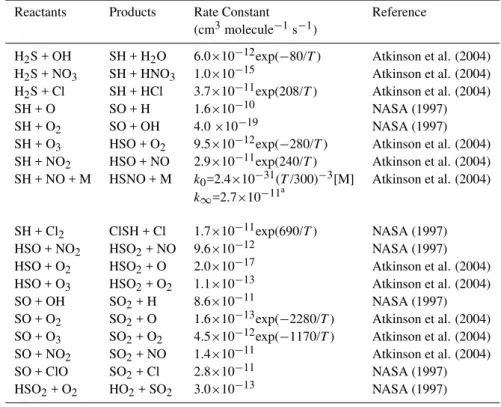
Table 2.Reactions added to CB05 for inorganic sulfur species and their reaction products.
Reactants Products Rate Constant Reference (cm3molecule−1s−1)
H2S + OH SH + H2O 6.0×10⁻¹²exp(−80/T) Atkinson et al. (2004) H2S + NO3 SH + HNO3 1.0×10⁻¹⁵ Atkinson et al. (2004) H2S + Cl SH + HCl 3.7×10⁻¹¹exp(208/T) Atkinson et al. (2004) SH + O SO + H 1.6×10⁻¹⁰ NASA (1997) SH + O2 SO + OH 4.0×10⁻¹⁹ NASA (1997) SH + O3 HSO + O2 9.5×10⁻¹²exp(−280/T) Atkinson et al. (2004) SH + NO2 HSO + NO 2.9×10⁻¹¹exp(240/T) Atkinson et al. (2004) SH + NO + M HSNO + M k0=2.4×10⁻³¹(T/300)−3[M] Atkinson et al. (2004)
k∞=2.7×10⁻¹¹ a
SH + Cl2 ClSH + Cl 1.7×10⁻¹¹exp(690/T) NASA (1997) HSO + NO2 HSO2+ NO 9.6×10⁻¹² NASA (1997) HSO + O2 HSO2+ O 2.0×10⁻¹⁷ Atkinson et al. (2004) HSO + O3 HSO2+ O2 1.1×10⁻¹³ Atkinson et al. (2004) SO + OH SO2+ H 8.6×10⁻¹¹ NASA (1997) SO + O2 SO2+ O 1.6×10⁻¹³exp(−2280/T) Atkinson et al. (2004) SO + O3 SO2+ O2 4.5×10⁻¹²exp(−1170/T) Atkinson et al. (2004) SO + NO2 SO2+ NO 1.4×10⁻¹¹ Atkinson et al. (2004) SO + ClO SO2+ Cl 2.8×10⁻¹¹ NASA (1997) HSO2+ O2 HO2+ SO2 3.0×10⁻¹³ NASA (1997)
aTermolecular rate constant expression:k=h k0
1+(k0/ k∞)
i
produces HSNO and reaction with Cl2produces ClSH. Both HSNO and ClSH can be treated as termination products.
SO Reactions: data on reactions of SO with OH, O2, O3, NO2and ClO have been reported and all produce SO2 (NASA, 1997). The reaction with O2is the slowest, but the abundance of O2makes it important relative to the other re-actions. ClO is a product of the reaction between Cl and O3.
HSO Reactions: Atkinson et al. (2004) report kinetic rate constants for HSO reactions with O2, O3, NO and NO2. As with other species, the reaction with O2 is the slowest but the abundance of atmospheric O2makes it important. HSO reacting with NO is also very slow compared to the other reactions and is not given further consideration. The reaction of HSO + NO2may produce HSO2+ NO (NASA, 1997) and these products were adopted for use here. HSO reacting with O2and O3are assumed to produce HSO2by analogy with the products of the NO2reaction. The only reaction identified for removing HSO2is that with O2, but it is fairly rapid given the levels of O2.
DMS Reactions: a realistic treatment of organic sulfur (Sorg) compounds must consider their reactions with vari-ous atmospheric oxidants. Finlayson-Pitts and Pitts (2000) provide a detailed overview ofSorg atmospheric chemistry. There is still much that needs to be learned about the kinet-ics and reaction products forSorg species. Studies have re-vealed that DMS is relatively reactive with a broad spectrum of chemical species, including O3, OH, HO2, O, Cl, ClO, IO, BrO, F, NO3, and N2O5. Ubiquitous O3 reacts slowly with DMS (rate constantk <1×10⁻¹⁸cm3molecule−1s−1). A comparative analysis of the various reactions reveals that DMS reactions with O, Cl, OH, OH + O2, and NO3 most likely control the fate of DMS in the atmosphere. Reac-tions with other halogen compounds are probably also im-portant in selected situations but little is known about natu-rally occurring emissions and atmospheric levels of species like IO and BrO. Noteworthy is the dual-channel reaction of DMS (CH3SCH3)with Cl with a rate constant of about 3.3×
10−10cm3molecule−1s−1 at 298 K and 1 atm (Finlayson-Pitts and (Finlayson-Pitts, 2000):
Cl+CH3SCH3→HCl+CH3SCH2 (R2)
→CH3S(Cl)CH3 (R3)
The reaction of OH with DMS is perhaps the most studied of all reactions involving DMS and it is one of the most com-plex. This reaction also occurs by way of two reaction chan-nels:
OH+CH3SCH3→CH3SCH2+H2O (R4)
OH+CH3SCH3+M↔CH3S(OH)CH3+M. (R5) At 298 K and 1 atm Reaction (R4) is predominant but Reac-tion (R5) becomes more important as temperature decreases. The first channel (Reaction R4) can be modeled directly fol-lowing Atkinson et al. (2004). In Reaction (R5) the OH
adduct itself may decompose back to its original reactants or it can react with O2to form DMSO [CH3S(O)CH3]: CH3S(OH)CH3+O2→CH3S(O)CH3+HO2. (R6) The chain of reactions that begins with Reaction (R5) and the formation of the OH adduct can be treated following Zhu et al. (2006):
DMS+OH+O2→0.5 DMSO+0.2 DMSO2+0.3 MSIA.(R7) Another DMS oxidation pathway is DMS+O which yields CH3SO and a methyl radical (Atkinson et al., 2004). The reaction of DMS + NO3may be important at night and yields CH3SCH2and nitric acid.
Table 3 lists the subset of Sorg reactions described here including oxidation reactions of DMS. Compromises and assumptions are necessary to treat some of the reactions and/or byproducts due to incomplete knowledge and the vari-ous assumptions are explained. Reactions involving halogen species other than chlorine are problematic to treat at this time because of uncertainties about their emissions.
CH3SCH2(MSCH2) Reactions: this radical is formed by three of the five DMS reactions. Its primary reaction path-ways are with O2and NO3. The reaction with O2is
CH3SCH2+O2+M→CH3SCH2OO+M (R8)
and the peroxyl radical CH3SCH2OO is subsequently de-noted MSP. Products of MSCH2 + NO3 are not known and are assumed, analogous to the companion reaction with O2, to be MSP and NO.
MSP Reactions: this mechanism includes three reactions involving MSP as a reactant. One is the reaction of MSP with itself. The other two are MSP with NO and MSP with HO2. MSP reactions with itself and other species are believed to form CH3SCH2O which is very unstable and rapidly de-composes to CH3S and HCHO. Thus, all reactions involving MSP can be treated as yielding products CH3S, HCHO and, in the case of MSP + NO, NO2.
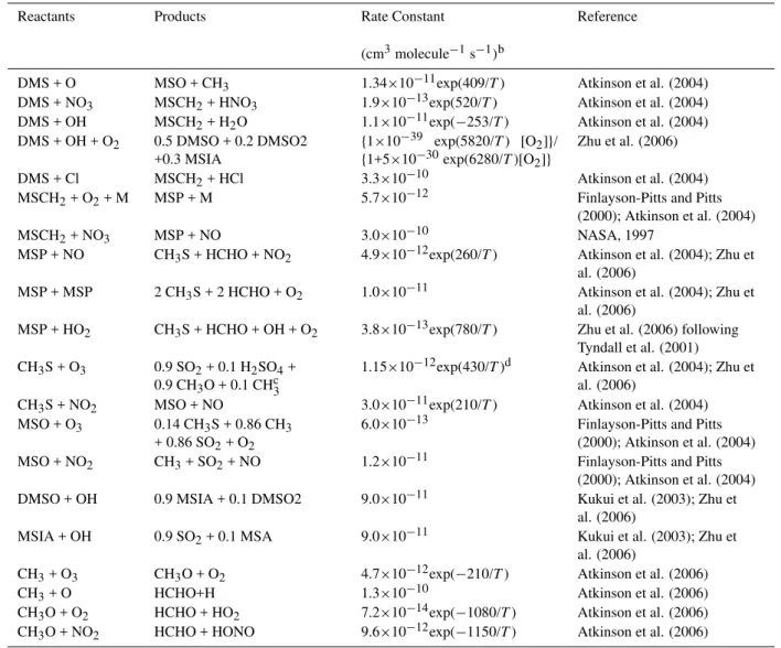
Table 3.Reactions added to CB05 for organic sulfur species and their reaction productsa.
Reactants Products Rate Constant Reference
(cm3molecule−1s−1)b
DMS + O MSO + CH3 1.34×10⁻¹¹exp(409/T) Atkinson et al. (2004) DMS + NO3 MSCH2+ HNO3 1.9×10⁻¹³exp(520/T) Atkinson et al. (2004) DMS + OH MSCH2+ H2O 1.1×10⁻¹¹exp(−253/T) Atkinson et al. (2004) DMS + OH + O2 0.5 DMSO + 0.2 DMSO2
+0.3 MSIA
{1×10−39 exp(5820/T) [O2]}/
{1+5×10⁻³⁰exp(6280/T)[O2]}
Zhu et al. (2006)
DMS + Cl MSCH2+ HCl 3.3×10⁻¹⁰ Atkinson et al. (2004) MSCH2+ O2+ M MSP + M 5.7×10⁻¹² Finlayson-Pitts and Pitts
(2000); Atkinson et al. (2004) MSCH2+ NO3 MSP + NO 3.0×10⁻¹⁰ NASA, 1997
MSP + NO CH3S + HCHO + NO2 4.9×10⁻¹²exp(260/T) Atkinson et al. (2004); Zhu et al. (2006)
MSP + MSP 2 CH3S + 2 HCHO + O2 1.0×10⁻¹¹ Atkinson et al. (2004); Zhu et al. (2006)
MSP + HO2 CH3S + HCHO + OH + O2 3.8×10⁻¹³exp(780/T) Zhu et al. (2006) following Tyndall et al. (2001) CH3S + O3 0.9 SO2+ 0.1 H2SO4+
0.9 CH3O + 0.1 CHc3
1.15×10⁻¹²exp(430/T)d Atkinson et al. (2004); Zhu et al. (2006)
CH3S + NO2 MSO + NO 3.0×10⁻¹¹exp(210/T) Atkinson et al. (2004) MSO + O3 0.14 CH3S + 0.86 CH3
+ 0.86 SO2+ O2
6.0×10⁻¹³ Finlayson-Pitts and Pitts (2000); Atkinson et al. (2004) MSO + NO2 CH3+ SO2+ NO 1.2×10⁻¹¹ Finlayson-Pitts and Pitts
(2000); Atkinson et al. (2004) DMSO + OH 0.9 MSIA + 0.1 DMSO2 9.0×10⁻¹¹ Kukui et al. (2003); Zhu et
al. (2006)
MSIA + OH 0.9 SO2+ 0.1 MSA 9.0×10⁻¹¹ Kukui et al. (2003); Zhu et al. (2006)
CH3+ O3 CH3O + O2 4.7×10⁻¹²exp(−210/T) Atkinson et al. (2006) CH3+ O HCHO+H 1.3×10⁻¹⁰ Atkinson et al. (2006) CH3O + O2 HCHO + HO2 7.2×10⁻¹⁴exp(−1080/T) Atkinson et al. (2006) CH3O + NO2 HCHO + HONO 9.6×10⁻¹²exp(−1150/T) Atkinson et al. (2006) aAbbreviations: DMS = dimethylsulfide, CH
3SCH3; DMSO = dimethylsulfoxide, CH3S(O)CH3; DMSO2 = dimethylsulfone, CH3S(O)(O)CH3; MSCH2 = methylthiomethyl
radical, CH3SCH2; MSP = methylthiomethylperoxyl radical, CH3SCH2OO; MSO = methylsulfoxide radical, CH3SO; MSIA = methanesulfinic acid, CH3SOOH;
MSA = methanesulfonic acid, CH3S(O)(O)OH.
bThe exception is for termolecular rate constants that have units of cm6molecule−2s−1. cThe mechanism of Zhu et al. (2006) treats the reaction of CH
3S with a variety of species as one reaction producing sulfur dioxide and sulfuric acid with no additional products
specified. As implemented in CMAQ, the additional products are assumed to be species needed to achieve stoichiometric closure to the reaction in the presence of H2O. dThis is believed to be a termolecular reaction (Atkinson et al., 2004) but the rate constant at different pressures has not been determined. See the text for further discussion.
single net reaction for CH3S with a host of ambient species as follows:
CH3S−−−−−−−−−−−−−−NO2,O2,HO2,O3,H2O→0.9SO2+0.1H2SO4 (R9) In addition, they assigned this a rate constant of 5.0 cm3molecule−1s−1 assuring a near instantaneous reac-tion. In light of data in Atkinson et al. (2004), and given the thermal instability of the CH3SOO product, we choose to ig-nore the reaction of CH3S with O2. The reaction CH3S+NO produces CH3SNO, but it was not included here because it photodissociates back to CH3S and NO during daytime
resulting in a fairly short lifetime and limited presence in the atmosphere. Clearly, this is one area where future ad-vances may require significant revision to the mechanism. The reaction with O3follows the net yield modeled in Zhu et al. (2006), but applies the measured rate constant in Atkinson et al. (2004).
– yielding CH3S and CH3+ SO2 (Table 3) – have partial yields that may be modeled based on data cited by Finlayson-Pitts and Finlayson-Pitts (2000). Finally, MSO + NO2is well character-ized and relatively fast.
DMSO & MSIA Reactions: DMSO reacts rapidly with O2 to form DMSO2 (Table 3). Zhu et al. (2006) relied on data from Kukui et al. (2003) to model the reactions of DMSO and MSIA with OH. Their simplifications reduce a complex set of reactions into two simplified reactions that were adopted in this study (k=9.0×10⁻¹¹cm3molecule−1s−1for both):
DMSO+OH→0.9MSIA+0.1DMSO2 (R10)
MSIA+OH→0.9SO2+0.1MSA (R11)
The net effect of the organic sulfur reaction set that starts with DMS is the production of inorganic species SO2 and H2SO4, along with organic species DMSO, DMSO2, MSIA and MSA. A number of reactions involving DMS, DMSO, DMSO2 and MSIA occur in clouds.
CH3 and CH3O Reactions: reactions involving the rad-icals CH3 and CH3O (produced from reactions previously described) are mentioned here for completeness. The chem-istry of these species is well characterized. CH3reacts fairly quickly with O and O3to produce CH3O. CH3O reacts with O2 to produce HCHO and HO2, and with NO2 to yield HCHO and HONO.
Heterogeneous (Cloud) Chemistry: in their ADOM model, Karamchandani and Venkatram (1992) used a heterogeneous chemistry approach similar into that in RADM/CMAQ al-though their treatment of cloud microphysics was more so-phisticated. A cloud model developed by de Valk and van der Hage (1994) for use in long range transport models also used relatively sophisticated cloud microphysics but its chemistry only treated the oxidation reactions of S(IV) by O3and H2O2. M¨oller and Mauersberger (1992) examined cloud chemistry from the opposite perspective, using sophis-ticated heterogeneous chemistry (57 aqueous reactions and equilibria) in a flow-through reactor-type model to examine the roles of various inorganic and organic reactants in sul-fur oxidation and radical cycling. Their sulsul-fur chemistry in-cluded S(IV) oxidation by O3, H2O2, organic peroxides, OH, NO3and metal ion catalysis, but no organic sulfur reactions. In addition, they simulated the interplay between OH, H2O2, HO2, O3, NO3and soluble organic species in cloud droplets. Under certain conditions (especially low SO2), clouds can be a net source of HO2 which can be transferred into the gas phase from the droplets. At very low SO2(<0.1 ppbV) no net H2O2 destruction (because of in-cloud H2O2 forma-tion) was computed, although clouds become a very effective sink for H2O2 when SO2>0.5 ppbV. M¨oller and Mauers-berger (1992) concluded that, in low SO2conditions, clouds play an important role in photooxidant dynamics.
Williams et al. (2002) used a one-dimensional cloud model to investigate the role of marine stratocumulus clouds as a possible source of HONO. Their calculations, based on a cloud model originated by Van den Berg et al. (2000), sim-ulated aqueous chemistry following the CAPRAM reaction mechanism (Herrmann et al., 2000) involving 86 species and 178 reactions. Williams et al. (2002) added 26 reactions treating reactive halogen species but simplified other reac-tions involving peroxy radicals. Their results indicated that in-cloud HONO formation, and its effects on droplet acid-ity and ozone chemistry, is most likely to be important in a moderately-polluted marine environment. However, due to large uncertainties in the aqueous chemistry involved, the modest impact on photochemistry and the high computa-tional requirements of the modified mechanism, they recom-mended against trying to incorporate HNO4/HONO istry into larger-scale three-dimensional atmospheric chem-istry models. Global modeling of sulfate and nitrate aerosols by Park et al. (2004) using their GEOS-Chem model com-puted in-cloud SO2oxidation by O3and H2O2at an assumed droplet pH of 4.5. They computed gas phase oxidation of DMS with yields of MSA and SO2but did not include DMS or MSA in the heterogeneous reactions.
Henze and Seinfeld (2006) reported increases in sec-ondary organic aerosol (SOA) formation from isoprene when using a parameterized aerosol formation mechanism in GEOS-Chem. Recently, Ervens et al. (2008) examined the formation of SOA by way of heterogeneous reactions involving organic compounds derived from isoprene. Two processes were modeled for producing aerosol mass from isoprene oxidation products by partitioning semivolatile organics between the gas and condensed phases using empirical partitioning ratios and modeling heterogeneous chemical reactions involving water-soluble isoprene oxi-dation products. The carbon aerosol yield was significant (to greater than 10% on the initial isoprene carbon mass in boundary layer cycling through clouds) and was dependent on the VOC/NOx ratio. Their heterogeneous chemistry model included over 40 reactions to simulate the evolution of inorganic sulfur and organic reactants that leads to sulfate and water soluble SOA products. The release of CMAQ version 4.7 (denoted “CMAQ4.7”) includes an update to the cloud chemistry that incorporates in-cloud SOA formation pathways originating with glyoxal and methyl-glyoxal (http://www.cmascenter.org/help/documentation. cfm?MODEL=cmaq\&VERSION=4.7\&temp id=99999). Thus, there is a need to follow up this current effort based on CMAQ4.6 by selectively adding organic reactions that produce SOA.
Early work performed under the National Acid Precipi-tation Assessment Program (NAPAP) of the 1980s (NAPAP, 1991) produced a simple cloud chemistry modeling approach within the larger RADM atmospheric chemistry model. The RADM module treated 5 reactions involving SO2oxidation by H2O2, S(IV) (=SO2(aq)+ HSO−3 + SO
2−
HSO−3 oxidation by peroxyacetic acid (PAA) and methyl-hydrogen peroxide (MHP), and S(IV) catalytic oxidation by Fe2+ and Mn2+. This approach was adapted as the default CMAQ cloud chemistry module (CCM). It assumes steady-state in-cloud conditions during the time integration of the ki-netic equations, with gas-aqueous equilibria computed using Henry’s Law constants for SO2, H2SO4, CO2, NH3, HNO3, O3, H2CO2(formic acid), H2O2, HCl, PAA, and MHP.
Following the approach of Zhu (2004) and Zhu et al. (2006), it is clear that there are a number of aqueous-phase chemical reactions involving DMS and its derivatives that lead to sulfate aerosol formation and should be added to complement the gas-phase reactions involvingSorg. The most important of these are:
DMS(aq)+O3(aq)→DMSO(aq)+products (R12)
DMS(aq)+OH(aq)→DMSO(aq)+products. (R13)
The principal aqueous reactions of DMSO are
DMSO(aq)+OH(aq)→MSIA(aq)+CH3(aq) (R14)
DMSO(aq)+SO−4(aq)→CH3SO
− 2(aq)+SO
2− 4(aq)+2H
+
(aq). (R15)
Details of these and other aqueous reactions are listed in Table 4. Reactions involving DMSO, DMSO2, MSIA, MSA and related species are also known to produce sulfate.
The most likely source of Cl and Cl−2 in cloud droplets is not from gas phase Cl – which is highly reactive and only expected to exist in air at extremely low concentrations – but HCl. The latter goes readily into solution where it dissociates as HCl→H++ Cl−. In the presence of the sulfate radical, SO−4(aq)+Cl−(aq)→SO2−4(aq)+Cl(aq) (R16)
(Zhu, 2004) and [Cl]aq reacts with [Cl−]aq to produce [Cl−2]aq. Properties of SO−4 have been measured in the lab-oratory (Chawla and Fessenden, 1975; Huie and Clifton, 1990), and its role in heterogeneous chemistry is described later. Also important are the aqueous reactions
OH(aq)+Cl−(aq)→HOCl−(aq) (R17)
HOCl−(aq)+H+(aq)→Cl(aq)+H2O. (R18)
Thus, [Cl]aq is affected by [SO−4]aq and [Cl−]aq. Zhu (2004) set [SO−4]aq, [Cl]aqand [Cl−2]aqto constant val-ues in his model. Chlorine’s role in the heterogeneous chem-istry of sulfate formation depends on the presence of the chloride ion and Zhu (2004) used the equilibrium relation
[Cl](aq)
Cl−(aq)
[Cl−2](aq) =7.14×10
−6
M (R19)
to compute the balance between Cl, Cl−and Cl−2 in droplets. Of the five DMSO oxidation reactions, those involving reac-tions with [Cl]aqand [Cl−2]aqare 2 to 4 orders of magnitude
slower than those in which [OH]aqand [SO−4]aqare reactants. Chlorine as Cl−2 can play a larger – though not dominant – role in reactions involving CH3SO−2. Hence, the role of chlo-rine in heterogeneous organic sulfur chemistry is of minor importance most of the time.
The reaction of DMS with OH (Reaction R13) is more than a factor of 20 faster than DMS with O3(Reaction R12) but O3 concentrations are far greater than OH making the ozone reaction the dominant pathway. For reactions with DMSO, the hierarchy of rate constants is kOH≈kCl> kSO−
4 ≫kCl −
2 ≫kO3. Ozone is the most abundant reactant to attack DMSO by at least 2 to 3 orders of magnitude. Nev-ertheless, the benefit of a higher concentration is still not suf-ficient to make up for its lower rate constant and the OH and SO−4 reactions with DMSO will usually be the most impor-tant.
It is clear from the work cited here that there are nat-ural emissions not treated in the standard SMOKE/CMAQ modeling package that are considered important on regional and global scales. Most notably, these omissions involve re-duced sulfur (especially DMS), NH3and water-soluble chlo-rine species from oceans, and LNOx. Despite the inherent uncertainty in quantifying these emissions, it is imperative to include them in any effort to examine a more complete pic-ture of how natural emissions influence air quality. Smith and Mueller (2010) describe in detail the methodologies used to add natural emissions to the standard SMOKE/CMAQ inven-tory. Data from the National Lightning Detection Network along with recent work estimating NOx production from lightning strokes formed the basis of LNOx emission esti-mates. Ammonia emissions from populations of large wild animals were included using estimates from US and Cana-dian wildlife inventories and emissions estimates for Mexico in the GEIA data base. Atmospheric chlorine is believed to play a role in ozone formation in coastal areas (Knipping and Dabdub, 2003) and provides radicals that may also contribute to aerosol formation in clouds. Effective emissions rates for HCl and nitryl chloride (ClNO2) in the marine boundary layer were incorporated from the GEIA data base, as were ammonia emissions from the oceans.
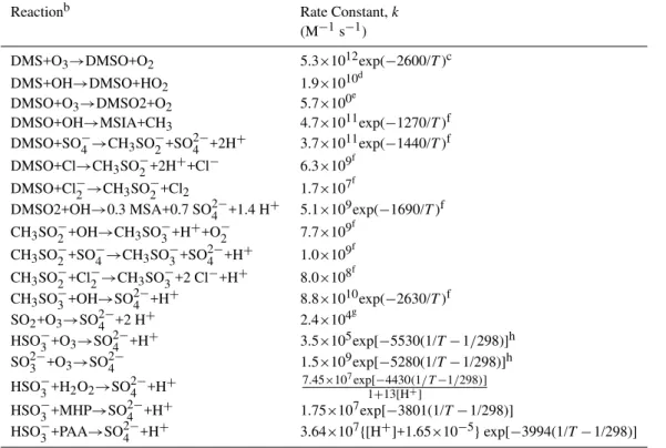
Table 4.Revised set of heterogeneous cloud reactions in CMAQ4.6.a.
Reactionb Rate Constant,k
(M−1s−1)
DMS+O3→DMSO+O2 5.3×10¹²exp(−2600/T)c DMS+OH→DMSO+HO2 1.9×10¹⁰
d
DMSO+O3→DMSO2+O2 5.7×100 e
DMSO+OH→MSIA+CH3 4.7×10¹¹exp(−1270/T)f DMSO+SO−4→CH3SO−2+SO42−+2H+ 3.7×10¹¹exp(−1440/T)f DMSO+Cl→CH3SO−2+2H++Cl− 6.3×10⁹f
DMSO+Cl−2→CH3SO−2+Cl2 1.7×10⁷ f
DMSO2+OH→0.3 MSA+0.7 SO2−4 +1.4 H+ 5.1×10⁹exp(−1690/T)f CH3SO−2+OH→CH3SO−3+H++O−2 7.7×10⁹
f
CH3SO−2+SO −
4→CH3SO−3+SO 2−
4 +H+ 1.0×10⁹ f
CH3SO−2+Cl−2→CH3SO−3+2 Cl−+H+ 8.0×10⁸ f
CH3SO−3+OH→SO2−4 +H+ 8.8×10¹⁰exp(−2630/T)f SO2+O3→SO2−4 +2 H+ 2.4×10⁴g
HSO−3+O3→SO2−4 +H+ 3.5×10⁵exp[−5530(1/T−1/298)]h SO2−3 +O3→SO2−4 1.5×10⁹exp[−5280(1/T−1/298)]h HSO−3+H2O2→SO2−4 +H+
7.45×10⁷exp[−4430(1/T−1/298)] 1+13[H+]
HSO−3+MHP→SO2−4 +H+ 1.75×10⁷exp[−3801(1/T−1/298)]
HSO−3+PAA→SO2−4 +H+ 3.64×10⁷{[H+]+1.65×10⁻⁵}exp[−3994(1/T−1/298)] aCMAQ species abbreviations: MHP = methylhydrogen peroxide; PAA = peroxyacetyl acid.
bThe last six reactions are essentially those treated in the standard version of CMAQ, although their rate constants were taken from other sources except for the last two which are
the expressions forkused in CMAQ.
cZhu (2004), Zhu et al. (2006), Gershenzon et al. (2001). dZhu (2004), Zhu et al. (2006), Bonifacic et al. (1975). eZhu (2004), Zhu et al. (2006), Lee and Zhou (1994). fZhu (2004), Zhu et al. (2006).
gZhu (2004), Zhu et al. (2006), Kreidenweis et al. (2003).
hZhu (2004), Zhu et al. (2006), Hoffman (1986), Kreidenweis et al. (2003).
phases. Section 2 (Methods) describes changes to both the CMAQ gas and cloud chemistry along with other aspects of an updated CCM. Results of CMAQ testing and simulations are reported in Sect. 3 followed by a summary with conclu-sions.
2 Methods
Version 4.6 was the most recent release of CMAQ at the out-set of this project. We used the CMAQ4.6 optional config-uration that includes an updated version of the carbon bond IV (CBIV) chemical mechanism denoted “CB05” (Yarwood et al., 2005). Because CMAQ is updated every 1–2 years it is impractical to try keeping up to date with the most current version, especially when independent model changes require extensive testing. One consequence of frequent code updates is that a more recent version often contains additional fea-tures or improvements that require further changes to ongo-ing work. CMAQ4.7 includes updates to the gas phase
Aside from chemistry, the CMAQ configuration applied here followed that used by the VISTAS Regional Planning Organization (see http://vistas-sesarm.org/) as described in Tesche et al. (2008). The VISTAS modeling domain covers all of the continental United States, large portions of Canada, Mexico, and adjacent ocean waters. The CMAQ parent grid over this domain is 4032 km (west-east)×5328 km (north-south) and composed of 36×36 km grid cells. Meteorolog-ical fields used by CMAQ are from simulations of the MM5 meteorological model (Grell et al., 1994). Chemical bound-ary conditions were derived from a 2002 global simulation using the GEOS-Chem model (Jacob et al., 2005).
2.1 Gas-phase chemistry modifications
The modified CB05 mechanism outlined here shares many similarities with, and borrows from, previously published work. Changes were made to the CMAQ4.6 CB05 gas-phase chemical mechanism to include reactive chlorine species, to add reactions for H2S and its derivatives, and to includeSorg chemistry. Reactions added to the CB05 mechanism were generally only those for which the products and kinetic rates are known and are sufficiently fast that they will have a sig-nificant impact on the evolution of atmospheric sulfur. Con-sideration was given to include those reactions that, although slow in comparison to competing daytime reactions, would be relatively important at night.
CMAQ4.6 has an option to include a set of gas-phase chlorine reactions in CB05, but it also in-cludes reactions involving hazardous air pollutants (http://www.cmascenter.org/help/model docs/cmaq/4.6/ HAZARDOUS AIR POLLUTANTS.txt). This CB05 enhancement was not used here because it required carrying a number of reactions that are not of interest for simulating natural ozone and aerosols. Instead, a subset of chlorine reactions originally added to the CMAQ4.6 CBIV reaction set (see Table 1, reactions attributable to Tanaka and Allen, 2001) were copied for use in CB05. Also added was Re-action (R1) previously described. These reRe-actions produce radicals (Cl, ClO, OH, HO2, XO2) that react with VOCs, NO, H2S, DMS and their oxidation products. Inorganic sulfur reactions added to CMAQ CB05 (see Table 2) include reactions of H2S with Cl, OH and NO3. Likewise, Table 3 lists all theSorgreactions added to the gas-phase mechanism and described previously. The Sorg reaction set is similar to that of Yin et al. (1990) and Zaveri (1997) with one major deviation: the CMAQ version omits the CH3SO2 and CH3SO3species and their reactions. The rationale for this is as follows. The simpler Zaveri mechanism has 11 reactions with CH3SO2as a product. In addition, it includes 12 reactions that involve CH3SO2or CH3SO3as reactants. Thus, 23 reactions are used by Zaveri (1997) to handle these two species. It is not possible to eliminate all these reactions (some are slow enough to neglect), but in all cases reactions forming CH3SO2can be replaced by reactions that
yield CH3+SO2 if we assume the thermal decomposition of CH3SO2 is fast in comparison with CH3SO2 chemical reactions. The generic SMVGEAR solver implemented in CMAQ was selected to calculate the time evolution of gas mixing ratios. This was necessary because the default optimized solver associated with the CB05 mechanism does not work correctly when changes are made to the reaction set.
2.2 Heterogeneous chemistry
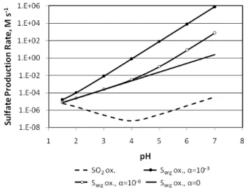
considerations). This is what is done in the revised CMAQ CCM in which [SO−4]=α{[HSO−3] + [HSO−4]},α≤1×10⁻³. Figure 1 illustrates the sensitivity of heterogeneous [SO2−4 ]aq formation to α and cloud droplet pH at a temperature of 298 K and pressure of 1 atm. In this ex-ample atmospheric mixing ratios were SO2=0.4 ppbV, DMSO=DMSO2=MSIA=MSA=0.1 ppbV,
O3 = 30 ppbV, H2O2=MHP=PAA=0.1 ppbV and OH=1×10⁻¹⁰ppbV, and cloud liquid water content (Wc) was 0.5 g m−3. When pH is ≤1.5, steady-state sulfate formation rates from organic and inorganic sulfur oxidation are within a factor of 10. However, the rates diverge rapidly as pH increases for all values ofα so that at pH=7 sulfate formation from oxidizedSorg exceeds that from SO2 by 5 orders of magnitude in the absence of [SO−4]aq and much more when [SO−4]aq>0. Note that, in the presence of anthropogenic sources, atmospheric levels of DMS and its oxidation products are much lower than SO2 but this is not necessarily the case in a simulation that examines the chemistry of “natural emissions” only. In addition, droplet pH is usually<5.6 unless there is a major nearby source of alkaline emissions. Thus, for expected droplet acidities, the influence of [SO−4]aqis small when its magnitude compared to HSO−3+HSO−4 is one ppm or less, but its importance grows rapidly with pH and for α above 1×10⁻⁶. Model sensitivity toαis explored in Sect. 3.
The dissociation of dissolved acids and bases – plus the presence of soluble salts (ammonium nitrate, sodium and potassium chloride, and magnesium and calcium carbonate) from airborne particles – contribute to an ion balance that de-termines droplet pH. Ion activity coefficients are computed to calculate the activities of all dissolved ionic species. The total rate of heterogeneous sulfate formation is computed as the sum of the rates of formation from the individual kinetic equations. Rate (transient) equations are integrated for 6-or 12-min periods followed by adjustments made to equilib-rium concentrations of interstitial gases and aerosol species consumed or produced during the integration. The CMAQ CCM is executed in a quasi steady-state manner with cloud chemistry pausing to allow gas chemistry to proceed before resuming the heterogeneous reactions. This method is used because it is simple to program, has low computational over-head and is easily modified. A disadvantage of this approach is that, by suspending gas-phase chemistry and diffusion dur-ing integration of the heterogeneous cloud reactions, it is likely that fast-reacting species will be depleted from the gas phase within the cloud, thereby stopping some heteroge-neous reactions (hence, the reason for CMAQ reducing the cloud integration time step from 12 to 6 min).
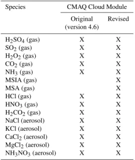
Table 5 lists the gas and aerosol species used to com-pute droplet acidity for both the CMAQ standard and re-vised versions of the CCM. The rere-vised CCM adds the ef-fects of MSIA and MSA on droplet acidity. Incorporating the reactions used by Zhu (2004) also requires the addition
α Χ
Χ Χ Χ Χ
Fig. 1. Comparative steady-state heterogeneous sulfate formation rates in the presence of SO2and equal parts DMSO and DMSO2 for different levels of [SO−4](aq) as determined from the
param-eter α. Atmospheric conditions are: 298 K, 1 atm, 0.5 µg m−3 cloud liquid water content,XSO2=0.4 ppbV,XDMSO=0.2 ppbV, XDMSO2=0.2 ppbV,XO3=30 ppbV,XOH=1×10
−10ppbV, to-tal peroxide=0.3 ppbV.
of Cl, Cl−2, SO−4 and OH as reactants in the revised CCM. As shown in the next section, Cl and Cl−2 are in equilib-rium with Cl− and this relationship is included in the ini-tial equilibrium calculation. The vapor pressure of H2SO4 over water is so low that it is assumed to be entirely ab-sorbed by cloud droplets. Initial cloud droplet equilibrium concentrations are computed by calculating the Henry’s Law aqueous concentrations of atmospheric gases (adjusting gas phase mixing ratios for highly soluble species), and solving a fourth-order equation in [H+]aq. Ion activity coefficients are subsequently calculated and ion aqueous activities are ad-justed accordingly.
2.3 Cloud chemistry mechanism
The rate at which droplets take up gaseous pollutants can be limited by gaseous diffusion toward the droplets and by the efficiency with which molecules of certain species pass through the gas-droplet interface. These rate-limiting pro-cesses are not treated by the default CMAQ CCM and have been added to the revised version. The following treatment is based on Seinfeld and Pandis (1998). Let the activity of water-soluble gas speciesiat the surface of a cloud droplet be denoted asCs(i). Diffusion limits both outside and within
the droplet and variations in chemical reaction times can re-sult in non-uniformCi throughout the droplet. This
charac-teristic of reactantCi directly affects the temporal evolution
of some species and must be treated in the chemical transient equations. The rate of change of the averageCi in a droplet
Table 5.Airborne chemical species ingested by clouds and used to compute droplet acidity.
Species CMAQ Cloud Module
Original Revised (version 4.6)
H2SO4(gas) X X SO2(gas) X X H2O2(gas) X X CO2(gas) X X NH3(gas) X X
MSIA (gas) X
MSA (gas) X
HCl (gas) X X HNO3(gas) X X H2CO2(gas) X X NaCl (aerosol) X X KCl (aerosol) X X CaCl2(aerosol) X X MgCl2(aerosol) X X NH3NO3(aerosol) X X
dCi
dt = xmt RT
pi−
Cs(i)
(HA)i
+X (1)
wherexmt is the mass transfer coefficient, R is the univer-sal gas constant, T is temperature, (HA)i is the Henry’s
Law constant,pi is the atmospheric partial pressure of the
species at a large distance from the droplet, andXis an aque-ous chemical reaction term representing any change due to chemical reactivity. To make (1) generic we replaceX with P
kl(QkPkl)−P j
QiLijwithPklrepresenting the
produc-tion rate of speciesifrom a reaction between specieskandl, andLijrepresenting the loss rate of speciesithrough its
re-action with speciesj. ParameterQ(defined below) is an ad-justment factor to account for the non-uniformity of a species activity,Ci orCk, within the droplet. Note that this assumes
co-reactant speciesCj andCl are uniform within the drop.
The transient equation then becomes dCi
dt = xmt(i)
RT
pi−
Ci
(HA)i
+X
kl(QkPkl)
−X
j QiLij
(2) wherexmtis given by
xmt(i)= "
rd2RT 3κg +
rd(2π MiRT )1/2
3ai
#−1
(3)
withκgas the gas diffusivity,Mi the molecular weight, and
ai the accommodation coefficient. The first product term on
the right hand side of (2) represents the diffusion and “stick-ing” tendency of speciesifrom the air surrounding a droplet
(with partial pressure differencepi−Ci /HA)to the droplet surface. The parameter ai is the ratio of the molecules of
speciesithat adhere to the droplet surface to the total num-ber of molecules that impact the droplet.
In Eq. (2), Qis the ratio of the average droplet activity of the non-uniform species to its activity at the droplet sur-face. When Q=1 the activity (concentration) is uniform. Chemical production and loss terms are derived from the ap-propriate kinetic rate equations. The backward Euler implicit method is used to solve for dCi
dt :
Cin+1=Cni +(Pn+1−Cin+1Ln+1)1t (4) (Seinfeld and Pandis, 1998). FunctionQis given by
Q=3
coth(q) q −
1 q2
,q=rd
kC U κw
1/2
(5) wherekis the reaction rate constant,CUrepresents the uni-form species activity, andκwis the water diffusivity (qandQ are dimensionless). In general,Q <1 whenkCU>108m−2 κw. If κw=1×10⁻⁹m2s−1 (1×10⁻⁵cm2s−1), then the co-reactant is non-uniform whenkCU>0.1 s−1. This im-plies that the non-uniform species is consumed by chemical reaction at a rate>10% per second.
Unlike in the default CMAQ CCM, this approach requires that droplet size be defined. Cloud droplets are assumed to be monodisperse (uniform in size) to minimize computer ex-ecution time. Measured droplet size distributions described by Byers (1965) for different cloud types – ranging from fog to stratus and convectively-growing cumulus and for 0.02 g m−3< Wc<0.8 g m−3 – were analyzed to estimate their median size characteristics. Median diameters for the analyzed droplet spectra ranged from 5 to 12 µm. Most val-ues ofWcprovided to the CCM are in the range represented by these median diameters, but higherWcare certainly pos-sible. As used here, whenWc≤1 g m−3the CCM calculated rdas
so that some dissolves into the aqueous phase but a consider-able amount remains in the gas phase. In addition, [HSO−3]aq and [SO2−3 ]aqare partly dependent on pH which tends to vary little during the period of integration ([H+]aqis treated as a steady-state species). Thus, for the short time interval when the transient equations are integrated any SO2and its deriva-tive ions consumed by chemical reactions are replaced by more SO2 from outside the cloud droplets. This allows the assumption that [SO2]aq, [HSO−3]aqand [SO2−3 ]aqare steady-state.
The steady-state assumption is strengthened by keeping the temporal integration interval short – currently ≤4 min – compared to the much longer temporal integration (6– 12 min) in the default CCM. Six to twelve minutes is long compared to some of the cloud chemical reaction rates but allowed for more computational efficiency. With faster com-puter processors it is now feasible to shorten the integration interval. The revised CCM uses a minimum integration step of one minute, the exact interval depending on the consump-tion rate of certain key species in the reacconsump-tion set. The max-imum interval of four minutes also allows for more frequent updating of gas phase chemistry so that some depleted reac-tive species in the air are allowed to recover more quickly between cloud chemical integrations than before.
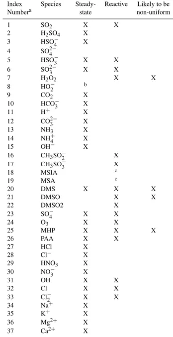
Table 6 lists all the species in the revised CCM, indicates which are treated as steady-state, which are reactive, and which are most likely to have non-uniform droplet concentra-tions. There are 8 species that are not steady-state and whose temporal changes are represented by transient equations. An analytical solution to this set of equations (see Appendix) is used to calculate changes in transient species.
2.4 Simulations
Comparisons between the old and new CCMs, and between different chemical pathways in the new CCM, provide in-sight into the effects of the new CCM on air quality sim-ulations. Most comparisons described here were done us-ing the natural emissions data set described by Smith and Mueller (2010), i.e., in the absence of anthropogenic emis-sions. CMAQ behavior in simulating sulfate aerosol was in-vestigated by exercising the model in various chemical con-figurations to identify its sensitivity to the gas-phase Sorg chemistry, cloud Sorg chemistry, cloud cover bias, and se-lected CCM parameters.
A series of CMAQ simulations (Table 8) were made us-ing a variety of model configurations so that a comparison of results from different simulations would provide insight into model behavior. Two simulations were made of the en-tire year using the fully-modified version of CMAQ4.6. One used the natural-only emissions data set and one used the total (natural plus anthropogenic) emissions data set. In ad-dition, several tests for June 2002 were made to investigate the influence of different gas and cloud chemistry options. June was selected because its intense photochemistry was
Table 6.Species treated in the revised CMAQ cloud module.
Index Species Steady- Reactive Likely to be Numbera state non-uniform
1 SO2 X X
2 H2SO4 X 3 HSO−4 X 4 SO2−4
5 HSO−3 X X 6 SO2−3 X X
7 H2O2 X X
8 HO−2 b
9 CO2 X
10 HCO−3 X
11 H+ X
12 CO2−3 X
13 NH3 X
14 NH+4 X
15 OH− X
16 CH3SO−2 X 17 CH3SO−3 X
18 MSIA c
19 MSA c
20 DMS X X X
21 DMSO X X
22 DMSO2 X
23 SO−4 X X
24 O3 X X
25 MHP X X X
26 PAA X X
27 HCl X
28 Cl− X
29 HNO3 X 30 NO−3 X
31 OH X X
32 Cl X X
33 Cl−2 X X
34 Na+ X
35 K+ X
36 Mg2+ X 37 Ca2+ X
aUsed as a subscript to identify species in the transient equations.
bAlthough linked to a species that is not steady-state, the activity of this species is only
determined for the purpose of computing the initial equilibrium cloud droplet acidity.
cThese species are not themselves reactive but dissociate to ions that are reactive.
All test simulations were based on natural-only emissions. Test simulation A used the standard (unmodified) version of CMAQ4.6. Test B used the model from test A but with the gas-phase chemical mechanism modified to include the addi-tional reactions described previously. Test C further modified CMAQ from test B by replacing the standard CCM with the modified version. Test D used the same version of CMAQ from test C but blocked cloud droplet uptake of OH, allow-ing a simulation of the effects of the modified CCM without the additional organic sulfur chemistry. Test E used the same test C CMAQ code but with artificially enhanced cloud cover over the Pacific Ocean to investigate the influence of clouds on sulfate formation from ocean sulfur emissions. Finally, test F also used the CMAQ version from test C but investi-gated model sensitivity to the sulfate radical proportionality factorαby increasing it from 1×10⁻⁶to 1×10⁻³.
3 Results
3.1 Grid-averaged model time series
Time series of simulated hourly natural pollutant concentra-tions for 2002, when averaged over the entire modeling do-main, provide insight into the joint behavior of emissions and secondary pollutants. Surface layer mixing ratios of selected gas species and aerosol concentrations were aver-aged for each hour and then a 24-h smoothing filter applied to suppress diurnal noise. Model output for 29 December 2001 through 10 January 2002 was dropped from the anal-ysis due to chemical spin-up issues. The simulation ended at 00:00 UTC on 1 January 2003 making 31 December in-complete (based on local time). Therefore, all 2002 results are presented for 354 days. Note that all time series plots in-clude “background” contributions from pollutants advected into the domain from the boundaries.
3.1.1 Photochemical species
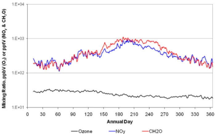
Figure 2 plots grid-averaged surface layer annual time se-ries of ozone, NOy(=sum of NO, NO2and all other model oxidized nitrogen species) and formaldehyde (CH2O). Both NOyand CH2O exhibit a clear winter minimum and summer maximum consistent with the expected seasonally-driven photochemical cycle. However, ozone is nearly constant for the first four months, declines slightly May through Septem-ber, and then levels off for the remainder of the year. Simu-lations made by removing lightning and wildfire NOx emis-sions revealed that the seasonal patterns of both sources fa-vor higher summer ozone and in no way contribute to the observed ozone pattern (the other source of natural NOx – soils – is too small to have a significant effect on the grid average). Thus, the winter/early spring peak in grid-average ozone is imposed on the grid from outside the modeling do-main, i.e., from the boundary conditions (BCs).
Fig. 2. Grid-averaged time series of three photochemically active species for the natural emissions simulation of 2002. Diurnal noise was removed by applying a 24-h averaging filter.
The global GEOS-Chem model, the source of these BCs, appears to produce a pattern of background ozone that is sim-ilar to that produced by Berntsen et al. (1999) except that their modeling also produced a summer minimum in back-ground air arriving in the US from across the Pacific Ocean. They concluded that the higher spring ozone was attributable to Asian emissions having a greater impact at long distances in spring because of enhanced trans-Pacific transport during that time of year. Vingarzan (2004) also found a spring (May) maximum in measured background ozone at “clean” sites in Canada and the US. Finally, Oltmans et al. (2008) analyzed ozone measured at west coast sites usually uninfluenced by air from the mainland, reporting an annual pattern for 2004 that looks a lot like the ozone pattern in Fig. 2 with a March– May peak.
across portions of the east where elevations are low. There is also strong evidence that the amount of pollutants trans-ported into the model domain across the boundaries is higher in winter and spring than in summer and autumn. Blaming all of the imported pollutants on transport from Asia is in-accurate, though. In fact, it appears that in April and May some of the extra ozone, especially across the southern and eastern US, is associated with pollution transported into the southern part of North America from Central America. En-hanced ozone is found along the southern model boundary reaching a peak monthly average of 33 ppb in April. In con-trast, ozone over the Pacific Ocean is at a maximum (30 ppb) in January, steadily decreases to a minimum in July (10 ppb) and recovers to values of 15–20 ppb in autumn. One enigma is the disparity in BC-derived ozone for January and Decem-ber. The December ozone plot was expected to look similar to that for January. However, December BC-derived ozone was much lower, especially over Canada and the US South-west, suggesting there was something different in the global meteorological patterns for January and December 2002 that significantly affected ozone formation and/or transport into North America.
3.1.2 Sulfur species
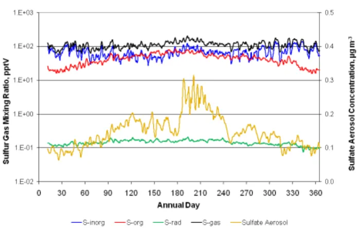
Time series of modeled sulfur (S) species are illustrated in Fig. 3. Inorganic S (Sinorg=SO2+ H2S + sulfuric acid) represents the most abundant class of gaseous sulfur com-pounds. Grid-average values peak above 100 pptV during several periods throughout the year. Grid-averageSorgstays below 100 pptV, peaking in summer and falling to levels well below those ofSinorgin winter. The S radicals (labeled “S-rad” in Fig. 3) time series is the sum of organic and inor-ganic gaseous S intermediate species (e.g., SH, HSO, CH3S and CH3SCH2)that are very reactive, have relatively short lifetimes and represent intermediate oxidation steps between DMS and H2S on one hand and MSIA, MSA, H2SO4 and sulfate on the other. S radical values peak in summer. The total gaseous S time series (“S-gas”) plotted in Fig. 3 indi-cates that the sum of all natural gaseous species tends to re-main fairly constant throughout the year with values in the 100–300 pptV range. Sulfate aerosol concentrations follow the expected seasonal cycle with grid-average values peak-ing near 0.3 µg m−3in summer.
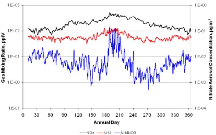
3.1.3 Nitrogen species
Ammonia, NOz(=NOy-NOx)and ammonium nitrate aerosol time series are plotted in Fig. 4. NOz, which includes ni-tric acid, represents the more oxidized of the nitrogen com-pounds and is a better indicator than NOxof precursors to nitrate aerosol formation. All these species follow a sea-sonal cycle with a grid-averaged summertime maxima. For NH4NO3 this represents a departure from the expectation that thermodynamics are more favorable for winter formation
Fig. 3.Grid-averaged time series of various gas and aerosol sulfur species for the natural emissions simulation of 2002. Diurnal noise was removed by applying a 24-h averaging filter.
of the aerosol. In both winter and summer, simulated natu-ral nitrate aerosol concentrations were primarily centered on areas with relatively high ammonia emissions. These areas were over the Pacific and Atlantic Oceans and the Gulf of Mexico, as well as in the vicinity of wildfires in the western US, Florida (winter), and eastern Canada (summer).
3.1.4 Particles
Figure 5 illustrates grid-averaged time series for all simulated natural particulate matter: sulfate, nitrate, estimated organic carbon (OC), elemental carbon (EC), fine soil dust, coarse particle mass (PMC=particles in the 2.5–10 µm diameter
range), fine sea salt and PM2.5(particles<2.5 µm). All ap-peared consistent with expectations based on seasonal emis-sions behavior and the dependence of atmospheric chemistry on meteorology. Ammonium sulfate/bisulfate, ammonium nitrate, and carbonaceous particles all peak in summer as does total PM2.5mass. Both fine dust and sea salt are highest in late winter and spring when winds are strongest. Coarse particles follow a similar pattern to that of fine dust.
3.2 Seasonally-averaged surface concentrations
Fig. 4. Grid-averaged time series of NOz, NH3and ammonium nitrate aerosol for the natural emissions simulation of 2002. Diurnal noise was removed by applying a 24-h averaging filter.
are much higher. These averages mask a great deal of spatial and temporal variability that is addressed by a future paper.
3.3 Influences of different gas and cloud chemistry treatments
Comparisons of test results from 11–30 June are provided in the following sections based on tests A through F.
3.3.1 Effect of adding reduced sulfur and chlorine gas phase chemistry: tests A and B compared
Differences between tests A and B reveal the impact of adding reduced sulfur and chlorine gas phase chemical re-actions to the standard CB05 mechanism. Changes are quan-tified as the mean change in variablex relative to reference variablex0[1¯ =(x−x0)/x0] for the entire period of the test simulations. The pattern in OH showed little change dur-ing the day with more significant changes at night. The re-sulting average over all June hours (Fig. 6, top) produced decreases over land as large as 60% and increases over the oceans of up to 60%. Nighttime increases over the water are almost certainly caused by the introduction of DMS and its derivatives. These species react with many other species that also react to remove OH. Thus,Sorg compounds act as an additional sink for species that remove OH thereby slow-ing the nocturnal depletion and resultslow-ing in higher nighttime levels. Widespread inland decreases in OH are the expected response to “agedSorg” (less DMS and more DMSO, etc.) in air advected across the continent from the west. Note that the aging ofSorgincludes formation of SO2.
The only source of secondary sulfate aerosols in standard CMAQ4.6 is SO2oxidation. The relative change in SO2due to the change in chemistry treatment is illustrated in Fig. 6 (middle). With meteorology fixed, the SO2response is deter-mined by SO2formation fromSorgoxidation and to a lesser extent by changes in OH, peroxides, and ozone.
Domain-Fig. 5. Grid-averaged time series of simulated particle concentra-tions for the natural emissions simulation of 2002. Diurnal noise was removed by applying a 24-h averaging filter.
wide SO2 increases occurred because of the organic sulfur chemistry added to the model. The largest increases – often 3 orders of magnitude and more – occurred over and down-wind of grid cells experiencing the highest emission rates of DMS and H2S. However, these dramatic increases are due in large part because many of the most affected grid cells have little or no SO2emissions.
Aerosol sulfate is enhanced everywhere by the chemistry changes (Fig. 6, bottom) but the greatest increases occurred near sources of DMS and H2S. Over many cells the increases exceeded a factor of 10. For ocean cells, sulfate averages increased by nearly 2 µg m−3 in some places. Inland sul-fate increases averaged 0.1–0.2 µg m−3over south Texas and Florida with smaller increases elsewhere.
3.3.2 Effect of adding organic sulfur cloud chemistry: tests B and C compared
Table 7.Average simulated winter and summer natural pollutant levels for the modeling domain.
Test CMAQ Configuration & Assumptionsa A Unmodified CMAQ4.6 using CB05 mechanism
B Test A configuration with CB05 mechanism modified to include DMS and H2S gas phase chemistry C Test B configuration with standard cloud module replaced by module that includes organic sulfur chemistry D Test C configuration but with OH cloud uptake blocked
E Test C configuration but with Pacific Ocean clouds enhanced between 250 and 750 mb F Test C configuration withα= 0.001c
aAll tests were run for the entire month of June.
bAll model layers in 250–750 m range included clouds with minimum cloud water content of 0.5 g m−3. cThe proportion,α, of [HSO−
3]aq+[HSO−4]aqin cloud droplets that is assumed to convert to the sulfate radical, SO−4. All other tests assumedα=1×10⁻⁶.
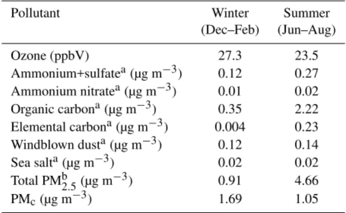
Table 8. Average simulated winter and summer natural pollutant levels for the modeling domain.
Pollutant Winter Summer (Dec–Feb) (Jun–Aug)
Ozone (ppbV) 27.3 23.5 Ammonium+sulfatea(µg m−3) 0.12 0.27 Ammonium nitratea(µg m−3) 0.01 0.02 Organic carbona(µg m−3) 0.35 2.22 Elemental carbona(µg m−3) 0.004 0.23 Windblown dusta(µg m−3) 0.12 0.14 Sea salta(µg m−3) 0.02 0.02 Total PMb2.5(µg m−3) 0.91 4.66 PMc(µg m−3) 1.69 1.05 aIn the fine particle size fraction (i.e., below 2.5 µm).
bAssumes organic aerosol mass equal to 1.8*OC.
reactions. Changes in SO2 (Fig. 7, middle) were negative over most of the domain. The SO2response to cloud chem-istry changes is caused by movingSorg from the gas phase where it oxidizes to SO2to the aqueous phase in which SO2 does not form.
Changes in aerosol sulfate in response to cloud chemistry changes (Fig. 7, bottom) occurred primarily where clouds were most prevalent. Significant reductions in sulfate from reduced SO2 gas phase oxidation was offset by enhanced sulfate formation in clouds. Widespread sulfate increases occurred over the Gulf of Mexico, Florida and the western Atlantic east of Florida where diagnostics indicate a persis-tent cloud cover for the month. Generally, the cloud chem-istry changes resulted in higher sulfate across the eastern half of the US. Sulfate increased over the Pacific Ocean off the North American coast by an average of 0.05–0.1 µg m−3 due to cloud chemistry but inland cloud effects were much smaller.
3.3.3 Effect of cloud OH uptake: tests D and B compared
Test D was done to determine the relative influence of the Sorg versus SO2 cloud chemistry as well as the differences between the old and new CCM SO2chemistry. The former comparison, enabled by not allowing OH to enter the clouds, was facilitated because aqueous OH reactions involvingSorg are the dominant reactions in the clouds (reactions involv-ing the sulfate radical and chlorine species were of much less significance because of the low value forα– see later com-parison of tests E and F). With both tests B and D using the modified gas phase chemical mechanism, their differences il-lustrate how the original and modified SO2cloud chemistry differentially influence sulfate formation.
Fig. 6. Mean simulated relative changes,1, during June in natu-¯ ral levels of airborne pollutants (top: OH; middle: SO2; bottom: aerosol sulfate) due to the introduction of reduced sulfur and chlo-rine gas chemistry into CMAQ4.6 (i.e., test B changes relative to test A). Model output is for the surface layer.
The different results between tests D and B are associated with differences in the behavior of the original and modified CCMs in their treatment of SO2chemistry (although some minor differences are caused by the reactions ofSorgas pre-viously mentioned). The revised CCM slows down SO2 re-actions by putting rate limits on droplet uptake of gaseous reactants and by computing average droplet concentrations (for fast-reacting species like H2O2)that are below the
ideal-Fig. 7.Same as in Fig. 6 except the changes represent the impacts from adding organic sulfur chemistry to the cloud chemistry module (i.e., test C changes relative to test B).