www.ann-geophys.net/26/3049/2008/ © European Geosciences Union 2008
Annales
Geophysicae
Blob formation and acceleration in the solar wind: role of
converging flows and viscosity
G. Lapenta1,2and A. L. Restante2,3
1Centrum voor Plasma-Astrofysica, Departement Wiskunde, Katholieke Universiteit Leuven, Celestijnenlaan 200B – bus 2400, 3001 Heverlee, Belgium
2Plasma Theory Group, Theoretical Division, Los Alamos National Laboratory, Los Alamos, NM 87545, USA 3Solar and Magnetospheric MHD Theory Group, Mathematical Institute, North Haugh, University of St Andrews, St Andrews, Fife KY16 9SS, Scotland, UK
Received: 20 September 2007 – Revised: 20 November 2007 – Accepted: 20 November 2007 – Published: 15 October 2008
Abstract. The effect of viscosity and of converging flows on the formation of blobs in the slow solar wind is analysed by means of resistive MHD simulations. The regions above coronal streamers where blobs are formed (Sheeley et al., 1997) are simulated using a model previously proposed by Einaudi et al. (1999). The result of our investigation is two-fold. First, we demonstrate a new mechanism for enhanced momentum transfer between a forming blob and the fast so-lar wind surrounding it. The effect is caused by the longer range of the electric field caused by the tearing instability forming the blob. The electric field reaches into the fast so-lar wind and interacts with it, causing a viscous drag that is global in nature rather than local across fluid layers as it is the case in normal uncharged fluids (like water). Second, the presence of a magnetic cusp at the tip of a coronal helmet streamer causes a converging of the flows on the two sides of the streamer and a direct push of the forming island by the fast solar wind, resulting in a more efficient momentum exchange.
Keywords. Solar physics, astrophysics, and astronomy (Corona and transition region; Magnetic fields) – Space plasma physics (Magnetic reconnection; Numerical simula-tion studies)
1 Introduction
The understanding of slow solar wind genesis has progressed considerably in the last few years following the observational discovery of plasma inhomogeneities (called blobs) formed and expelled from regions above coronal streamers (Shee-ley et al., 1997; Wang et al., 1998). The observational evi-dence has been provided by the Large Angle and Spectromet-ric Coronagraph (LASCO) instrument on the Solar and He-Correspondence to: G. Lapenta
liospheric Observatory (SOHO). LASCO comprises of three telescopes (C1, C2 and C3), each of which looks at an in-creasingly large area surrounding the Sun (Brueckner et al., 1995).
Approximately 4 blobs per day were observed in a rela-tively quiet period for the solar corona (year 1997, near solar minimum). After formation, the blobs are carried away with the ambient slow solar wind. Generally, the plasma blobs move radially outward with their speed increasing from 0– 250 km s−1in the region 2–6 R⊙(C2 field of view) to 200– 450 km s−1in the region 3.7-30 R⊙(outer portion of the C3 field of view). A possible interpretation is that the blobs form the slow solar wind as a superposition of many plasmoids of different sizes (Mullan, 1990).
Models of the formation of blobs have focused on mech-anisms involving reconnection between open field lines and closed field lines (Einaudi et al., 1999; Einaudi et al., 2001; Endeve et al., 2003; Fisk and Schwadron, 2001; van Aalst et al., 1999; Wang et al., 1998; Wu et al., 2000). Through field line reconnection, plasma from the denser regions within the helmet streamer is liberated and becomes tied to open field lines and forms the slow solar wind (Einaudi et al., 2001).
configurations atop the closed field lines in coronal stream-ers (Lapenta and Knoll, 2005).
The fundamental conclusion of the model by Einaudi et al. (1999) and in successive refinements is that a blob is formed by the tearing instability and that by virtue of the interaction with the fast solar wind the blob is accelerated and ejected, carrying with it the plasma that forms the slow solar wind.
The fundamental question posed by the present work is: “what is the basic physical process for the plasma accelera-tion”? We consider specifically two possibilities. First, that the momentum transfer causing the blob acceleration is due to viscous drag. Second, that the acceleration is due to the insurgence of the tearing instability and its non-linear ef-fects. The acute reader will not find the suspense spoiled by learning that, as usual, Nature turns out not to be black or white. We discover that both mechanisms are present in an interplay mediated by the electric field. Furthermore, the presence of the converging flows at the cusp of the coronal streamer causes a direct momentum transfer by the action of the plasma flowing against the forming island and pushing it upward from the solar surface.
The paper is organised as follows. Section 2 summarises the two initial configurations considered: the 1-D initial con-figuration proposed by Einaudi et al. (1999) and its 2-D ex-tension to include the presence of a magnetic cusp (Lapenta and Knoll, 2005). Section 3 very briefly provides the methodology for our investigation: the resistive MHD model as implemented in the FLIP3D-MHD code (Brackbill, 1991). Sections 4 and 5 present the non-linear evolution, respec-tively, of the case of the initial 1-D reversed field and of the 2-D configuration with a magnetic cusp. Conclusions are reached in Sect. 6.
2 Initial configuration
The region where the blobs are formed and presumably re-connection happens has been localised thanks to the LASCO observations. The blobs are formed between 2–3 R⊙ (the cusp region) and are accelerated afterwards, reaching termi-nal speed 250–450 km s−1 at 20–30 R⊙. The sonic point where the fast solar wind reaches sonic speeds is estimated at 5–6 R⊙, the Alfv´en point is further outwards (at around 10 R⊙). In the region of blob formation, the fast wind is slightly subsonic and definitely subAlfv´enic. In the present paper we consider the region where the plasma blobs and the slow so-lar wind originate. We consider the region below the Alfv´en critical point, near the cusp where we assume the plasma to be near sonic but subAlfv´enic.
We consider two types of configurations previously pro-posed for the region where blobs are observed to form. The first is 1-D and is a simple force-free extension of the Har-ris equilibrium (Einaudi et al., 2001). The second, is a more complex 2-D equilibrium representative of a Helmet streamer (Lapenta and Knoll, 2005). In both cases, the
cen-tral current sheet represents the area above the tip of a helmet streamer where the blobs have been observed to form in the LASCO images. To model the presence of the fast solar wind emanating from the coronal holes, the initial equilibrium in-cludes the presence of a flow along the field lines. The flow is chosen to be zero along the field lines directly above the streamer tip and to increase rapidly away from it, to reach an asymptotic value corresponding to the fast solar wind. The details of the initial configurations have been presented in previous publications and are summarised below for each of the two cases.
We use Cartesian coordinates whereyandzare parallel to the Sun’s surface (withzalong the meridians andyalong the equator) andx is orthogonal to and pointed away from the Sun’s surface.
2.1 1-D force-free equilibrium
We use the 1-D model proposed by Einaudi et al. (2001). The magnetic field is force-free (i.e. the pressure, temperature and density are uniform) and is given by
B0x=B0tanh((z−z0)/L)
B0y=B0sech((z−z0)/L) (1)
whereLis the length scale of the variation ofB. A plasma flow with a wake profile is chosen:
u0x(z)=u0sech((z−z0)/L); (2) The flow profile is chosen according to the model of Einaudi et al. (2001). The flow is idealized as it does not include the spherical geometry of the Sun and the progressive acceler-ation away from the Sun. However it includes the aspects of relevance here: it represents the shear betwen the fast so-lar wind propagating along the open field lines and the static plasma above the helmet streamer. As noted in Einaudi et al. (2001), the scale-length of variation of the flow shear might differ significantly from the length scale of variation of the magnetic field. However, for simplicity we assume them to be the same. In the present paper we follow the analysis of Einaudi et al. (1999); Einaudi et al. (2001) which estimated the particular caseu0/vA=2/3 (with the Alfv´en speedvAis defined withB0and with the uniform densityn0) to be rep-resentative of the realisitc conditions. The flow is compress-ible, with an ideal equation of state withγ=5/3.
Periodic boundary conditions are applied in thex direc-tion and free-slip boundary condidirec-tions are applied inz. The boundaries in z allow no outflow of plasma and form ef-fectively a closed plasma channel. A small perturbation is added to the system to stimulate the growth of any instability present. The perturbation is added to theycomponent of the vector potential as:
δAy=ǫsin(kxx)sin(kzz) (3)
2.2 2-D Helmet-streamer
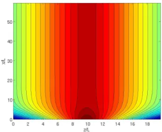
The second initial configuration is based on the work by Wiegelmann et al. (1998) where a magnetic field configu-ration with a current sheet typical of a helmet streamer is computed analytically. The equilibrium is rigourously exact only for infinitely stretched helmet streamers, but it can be used even for realistic aspect ratios as a good approximation. In the coordinate system used here, the current is initially directed alongyand the initial magnetic field is in the(x, z)
plane (see Fig. 1), withx being the direction away from the Sun’s surface.
The initial equilibrium is 2-D and is independent of they
coordinate. The initial configuration is characterised by the
ycomponent of the vector potential:
Ay(x, z)= − 2 clog cosh c r p0
2 (z−z0) +1 clog p0 k (4) wherec,z0andkare constants andp0(x)=s1e−s2x+s3The initial magnetic configuration has a current:
j = p0c
cosh2qp02c(z−z0)
(5)
and is held in pressure equilibrium by a pressure profile:
p= p0
cosh2 q
p0
2c(z−z0)
+pB (6)
The separatrices between open and closed field lines are po-sitioned symmetrically at equal distances from the centrez0:
zsep = 1 c s 2 p0 arctanh s p0−ς
p0 !
(7)
whereς=ke−cAs. In the simulations shown below we choose the parameters as in Wiegelmann et al. (2000, 1998); Lapenta and Knoll (2003):s1=.8,s2=4,s3=.2,c=15,As=.1073 and k=1, z0=1. Following Wiegelmann et al. (2000), a small (20%) background plasma pressurepB is added to simplify the numerical treatment. The initial configuration is assumed to have uniform plasma density and the specific internal en-ergy profile can be derived from Eq. (6):
I = p
ρ(γ −1) (8)
Additionally, we add an initial wake velocity field: u(z)=
1−sech
|z−z0| −zsep
Lv
e−|
z−z0|−zsep
2Lv bb (9)
wherebb is the unit vector in the direction of the magnetic field and Lv is the scale-size of variation of the velocity
Fig. 1. Initial Helmet Streamer equilibrium. Note that the vertical and horizontal axis are not on the same scale, the vertical axis is compressed.
field. The flow is present only outside of the two separatri-ces, where the field lines are open and is zero inside, where the field lines are closed.
At the bottom boundary (x=0), the field lines are tied and the flow and the plasma are continuously resupplied with the same value used for the initial condition to simulate the fast wind ejected from the coronal holes. At all other boundaries, open conditions are applied to allow the outflow of plasma.
Unlike the previous case, no initial perturbation is applied since the error in the approximation of infinite stretching typ-ical of the derivations leading to Eq. (4) is in itself a sufficient initial perturbation.
In the present 2-D equilibrium the equilibrium vary along
zand the typical thickness of the layer downstream of the cusp isL=Lz/20. As in the 1-D case, the velocity is assumed to have the same length scale as the magnetic field:Lv=L.
3 Simulation approach
The simulations for the present work are conducted with the FLIP3D-MHD code (Brackbill, 1991) based on the classic textbook viscous-resistive MHD model (see e.g. Goossens (2003)), comprising a mass continuity equation,
dρ
dt +ρ∇ ·u=0 (10)
Faraday’s and Ampere’s laws,
d dt B ρ
= Bρ · ∇u− 1
ρ[∇ ×ηJ] (11)
Ohm’s law,
E=ηJ−u×B (12)
a momentum equation,
ρdu dt = −∇
" p+ B
2
2µ0 #
+
∇ ·BBµ
0
− ∇ ·νρ5 (13)
and an energy equation,
ρdI
dt = −p∇ ·u+νρ(5·5)+η(J·J) (14)
whereρis the mass density, B is the magnetic field intensity, J is the current density,µ0is the magnetic permeability of vacuum, u is the fluid velocity,I is the specific internal en-ergy, andpis the fluid pressure. The symmetric rate-of-strain tensor,5, is defined in the usual way (Braginskii, 1965),
5= 1
2[∇u+ ∇u T
] (15)
The pressure is given by the equation of state,p=(γ−1)ρI
withγ=5/3. The transport coefficients are the kinematic shear viscosityν and the resistivityη. The solenoidal con-dition on B,
∇ ·B=0 (16)
is imposed throughout the evolution. As noted in the litera-ture, the effect of gravity can be neglected within the scope of the present paper aimed at understanding the magnetic pro-cesses responsible for the origin of blobs in the slow solar wind (Einaudi et al., 2001; Lapenta and Knoll, 2005).
The system under investigation is studied in a two-dimensional plane (x,z) using FLIP-MHD, a resistive MHD code described in Brackbill (1991). The system size in each direction is labelled Lx, Lz and a grid made of 300×600 Lagrangian markers is used in each direction arrayed ini-tially in a 3×3 uniform formation in each cell of a 100×200 grid. The units of the simulations are normalised to the mag-netic (and velocity) scale lengthL and to the Alfv´en time
τA=L/vA. The Lundquist number (Goedbloed and Poedts, 2004) is computed asS=µ0vAL/ηand the Reynolds number as:Rv =u0ρL/ν(using the initial uniform density and the fast solar wind speed). The adimensional numbers are de-fined using average quantities. Viscosity and resistivity are uniform and constant in time in all simulations reported be-low.
4 Non-linear evolution of the 1-D initial equilibrium
The initial state is characterised by both a flow shear and a magnetic shear. In principle, a number of instabilities could be present (Biskamp, 1997; Bettarini et al., 2006). However,
for the choice of parameters considered only two types of instabilities are present.
As shown in previously published results (Einaudi et al., 2001; Lapenta and Knoll, 2005), the resistive tearing insta-bility is present and grows at a rate determined by the re-sistivity of the system. The resistive tearing mode leads to the formation of a magnetic island that mixes outer and inner field lines. In the process, the outer solar wind can transfer its momentum to the inner plasma and produce a net motion of the tearing island. This process is clearly reminiscent of the observed formation of blobs and their subsequent accel-eration away from the Sun.
However, a second instability is present. Even in absence of resistive MHD modes, the viscosity is itself capable of al-tering the initial profile. Indeed, a viscous flow would tend to flatten any flow profile in time by virtue of direct viscous drag alone. The inner layer that is initially motionless would pro-gressively acquire speed (Landau and Lifshitz, 1959). In the corona, the viscosity is very low unless anomalous effects be-come important. However, in any realistically feasible sim-ulation, numerical viscosity has to be present to avoid the formation of small scale structures that cannot be resolved and would lead to numerical instabilities.
One aim of the present work is to elucidate the relative role of this second process relative to the first. The question is: is the slow solar wind acceleration observed in the simulations due to the tearing instability or to the viscous drag? And how does it scale with viscosity and resistivity?
4.1 Formation of the slow solar wind and of plasma blobs To exemplify the typical evolution observed in the simula-tions of the 1-D initial state, we report the results of a simu-lation for the particular case with Lundquist numberS=104 and viscous Reynolds numberRv=104.
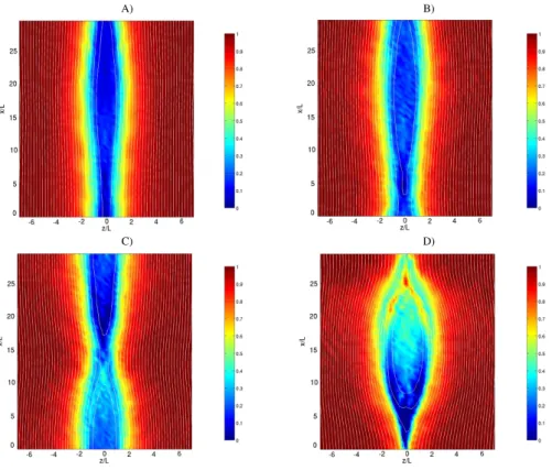
The initial phase of the evolution sees the formation of a magnetic island that perturbs the initial topology of the sys-tem and the initial flow profile. Figure 2 shows the velocity away from the Sun in false colour, superimposed on the mag-netic field lines, at four times showing different phases of is-land formation. The isis-land grows and moves away from its original formation site. Comparing the different times shown in Fig. 2 demonstrates that the island moves along with the flow. Note that in Fig. 2, the frame of reference is chosen stationary with the stagnant plasma, so the motion of the is-land seen in the figure is with respect to the solar frame of reference.
A) B)
C) D)
Fig. 2. Non-linear evolution of the initial force-free reversed field equilibrium. Velocity component (false colour) away from the Sun (in the frame of reference of the Sun) and magnetic field lines (white) are shown at four different times (A:t /τA=143, B:t /τA=215, C:t /τA=229,
D:t /τA=251) in a run withS=104andRv=104.
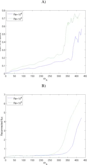
viscosity (Rv=103) but equal resistivity is also reported. The process of acceleration progresses in two steps. After a pro-gressive and continuous phase of acceleration of the initially stagnant plasma, a sudden acceleration develops when the island becomes so big as to feel the effect of the boundary conditions. As shown below, this last phase is only present in the low resistivity cases and it is due to a transition from a X-point reconnection process to a Y-X-point reconnection process with a progressively more elongated leg (Biskamp, 2000) becoming progressively more turbulent and undergoing sec-ondary island formation. These features of the reconnection mechanism are well known and will not be addressed here again, the interested reader is referred to the excellent text-book by Biskamp (2000).
The process of island formation is further shown in Fig. 4b where for the same two simulations, the reconnected flux is shown. The onset of the faster reconnection phase also is similarly due to the boundary conditions.
Figure 4 shows a comparison of two cases with different viscosity and demonstrates that indeed viscosity has a strong impact on both island formation and slow solar wind accel-eration. In the next paragraph this effect is further analysed.
4.2 Role of viscosity and resistivity
The behaviour displayed above is in agreement with previ-ously published results (Einaudi et al., 2001; Lapenta and Knoll, 2005) and it is reproduced primarily to provide the reader with a summary of the typical evolution. Below we investigate the main point of the present effort, namely the causes of the observed behaviour displayed in Fig. 3. Both the tearing instability and viscous stresses can be the cause: to determine which dominates, we change independently vis-cosity and resistivity. The tearing instability is proportional to resistivity, viscous drag is proportional to viscosity. We need to determine whether the momentum transfer is propor-tional to viscosity or resistivity.
Figure 5 shows the summary of the different runs con-ducted varying resistivity and viscosity. Each panel corre-sponds to a different resistivity and reports the time evo-lution of the maximum difference in the averaged profile
<ux(z)>x, corresponding to the differential between the flank velocity (fast solar wind) and the central plasma (slow solar wind). In each panel several runs are displayed, corre-sponding to different viscosities in each run.
A)
B)
Fig. 3. Evolution of the average velocity profile<vx(z)>x
(nor-malised to the asymptotic speedu0) for two runs starting from the
initial force-free reversed field equilibrium with the same resistiv-ity (S=104) but different viscosity (panel A withRv=104, panel B Rv=103).
presence. In some cases at lowRv, the system never reaches this state, at least before the completion of the run. While a quantitative investigation of this boundary effect might be of interest from the general perspective of reconnection physics, it will not be pursued here as boundary conditions are clearly not directly relevant to the real solar case. When the boundary conditions affect the evolution, it simply sig-nals the end of the relevance of the simulation to the practi-cal case of the Sun. Second, observing the progressive ac-celeration phase, one unmistakable conclusion emerges: the speed of acceleration (i.e. the slope of the curve in the fig-ures) is hardly affected by the resistivity but scales mono-tonically and markedly with the viscosity. The conclusion regarding the comparatively lower sensitivity of the accel-eration mechanism to resistivity was already discussed in a previous work (Lapenta and Knoll, 2005). Here the focus
A)
B)
Fig. 4. Evolution of the minimum of the average velocity (normal-ized to the asymptotic speedu0) minz(<ux(z)>x)(A) and of the
reconnected flux (B) for two runs starting from the initial force-free reversed field equilibrium with the same resistivity (S=104) but dif-ferent viscosity (panel A withRv=104, panel BRv=103).
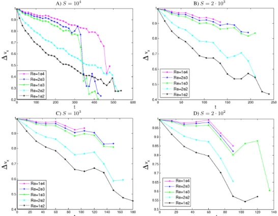
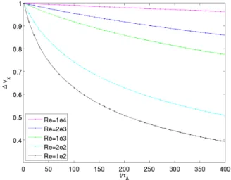
is on the much more apparent sensitivity to viscosity. As viscosity is increased by two orders of magnitude from a Reynolds number ofRv=104toRv=102, the slope increases markedly: for example, the speed at time oft /τA=200 for the runs withS=104drops by 10% in theRv=104case and 55% in theRv=102 case. Clearly the mechanism for slow wind acceleration appears to be more linked to the process of viscous drag than to the processes related to resistivity and island formation.
A)S= 104
B)S= 2·103
C)S= 103
D)S= 2·102
Fig. 5. Evolution of the difference1Vxbetween the maximum (fast solar wind) and minimum (slow solar wind) in the profile of the average
vertical velocity (normalized to the asymptotic speedu0). Several runs are shown starting from the same initial force-free reversed field
equilibrium, each panel corresponds to a different resistivity: (A)S=104, (B)S=2·103, (C)S=103and (D)S=2·102. In each panel 5 viscosities are shown, corresponding in order from the top curve to the bottom curve toRv=104,Rv=2·103,Rv=103,Rv=2·102,Rv=102.
4.3 Role of the electric field
A key aspect of the evolution of the system considered above rests in the role of the electric field. The initial equilibrium is already characterised by an electrostatic field needed to produce the velocity shear imposed initially. The subsequent evolution of the tearing mode leads to the growth also of an electromagnetic field.
In the present MHD treatment, the plasma flow is primar-ily due to the drift motion caused by the presence of electric fields:
vE×B=
E×B
B2 (17)
Once the electric field is written in terms of the vector po-tential A and the scalar popo-tentialϕ, the drift clearly shows the presence of a dual nature:
vE×B= −
1
B2(∇ϕ×B+
∂A
∂t ×B) (18)
The flow can be of two natures: electrostatic and electromag-netic. The initial configuration has only avx(z)component of the flow that is caused by aEzcomponent of the electric field: therefore the electric field has zero curl and it is purely electrostatic.
The tearing mode is a mode primarily involving the evolu-tion of the out of plane component of the vector potential A and it is inductive in nature since it produces an electromag-netic field thanks to the topological variations of B. However, in presence of out of plane components of the field, there is also an electrostatic potential associated with it (Daughton and Karimabadi, 2005).
The viscous effect alone, instead, does not directly affect the magnetic field and causes electrostatic fields. If we con-sider the evolution of the initial state under the action of vis-cosity alone, the full set of equations reduces to just:
∂ux ∂t = −
1
Rv ∂2ux
∂z (19)
governing the only remaining variableux(z). Using Ohm’s law, it follows:
because, similarly, B does not change along the flow lines. The variation of the velocity field generated by viscous drag causes an electric field with zero curl, i.e. it generates an elec-trostatic field.
The effect of viscosity alone can be computed easily by solving directly Eq. (19). As it is well known (Barenblatt, 1996), a linear diffusion equation like Eq. (19) admits a self-similar analytical solution of the form:
ux=u0 1
t1/2e−
Rvz2/4t (21)
that provides a simple scaling law for the time-variation of the differential in the speed of the central initially stagnant plasma and the outer fast solar wind:1Vx∝1/√t.
To illustrate the effect of viscosity alone, we have solved the equation for viscous drag (i.e. Eq. 19) numerically start-ing with the same initial profile considered in the full MHD simulations and for the same ranges of viscosity. Figure 6 shows the evolution in time of the jump in speed between the central plasma and the outer fast solar wind. The results can be compared directly with Fig. 5 for the full MHD simula-tions. As can be observed the additional effect of the pres-ence of the magnetic field evolution is very significant. The general shape of the time evolution is the same in the purely viscous case as in the full MHD case, and in both cases re-sembles the inverse-square-root power law predicted by the self-similar solution. A quantitative comparison reveals that the evolution with full MHD has a very much increased rate of decay. For example, considering the caseRv=103, at time t /τA=200, the full MHD simulation shows a difference in speed of 0.65, while in the purely viscous case this differ-ence is still 0.87. Clearly, the full MHD evolution provides additional drag forces that transcend the direct viscous drag.
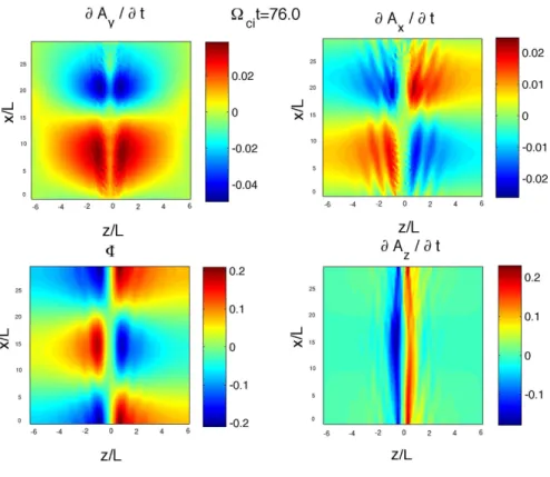
The additional force is coming from the electric field. Figure 7 shows the vector and scalar potential at time
t /τA=76, for the same simulation shown in Fig. 2 above. A significant electrostatic field is present form the beginning and it is caused, as noted above, by the need to support the initial sheared velocity field. The history of the electric field energy is shown in Fig. 8. The partial contribution of the electrostatic field is shown as a dashed line. Except for thez
component that includes the initial strong electrostatic field supporting the sheared flow, the electromagnetic component proper of the tearing mode dominates all components. The electric field perturbation is therefore primarily caused by the tearing growth and not by viscous drag.
The tearing instability developing in the centre of the sys-tem moves with respect to the plasma in the flanks as shown in Fig. 2. The island remain localised in the centre of the plasma and it comoves with the local plasma speed. The di-rect viscous drag is small. However the island’s electric field structure extends far beyond it and well into the flanks, as shown in Fig. 7. These fields move with the island speed and have a relative speed with respect to the fast solar wind in the
Fig. 6. Evolution of the difference in velocity1Vx between the
central plasma (initially at rest) and the outer fast solar wind. The results are from a simple purely viscous simulation that neglects any magnetic field and resistive effect. Five viscosities are shown, from top to bottom: Rv=104,Rv=2·103,Rv=103,Rv=2·102
andRv=102.
flanks. The expanded range of influence of the island deter-mined by the electric fields allows for an enhanced drag that no longer happens only across layers touching each other but extends globally as the electric field of the island feels the drag force over the whole domain.
5 Non-linear evolution of the initial 2-D helmet streamer equilibrium
The 2-D helmet streamer configuration considered is char-acterised by the presence of a cusp region above the helmet streamer where the field lines from converging towards the cusp at lower altitudes become essentially parallel. In this region the field-aligned speed also changes direction from a converging motion at lower altitudes to a parallel motion above. In the 1-D equilibrium considered above, the focus was entirely on the region above the cusp where the flow and filed lines are initially straight and parallel. The 2-D equilib-rium with cusp, instead, allows us to consider also the motion in the lower part where the flow and the field lines are con-verging.
Fig. 7. Scalar potential and the three components of the time derivative of the vector potential are shown in the four panels at timet=76 for a run starting from the initial force-free reversed field equilibrium withS=104andRv=104(same run considered in Fig. 2). The different
components are listed above each panel.
studied here, the flow toward the cusp produced a specific reconnection process. The speed of this reconnection pro-cess is proportional to the incoming flux. It is insensitive to the resistive processes that can break up the frozen-in con-dition (Lapenta and Knoll, 2005). As illustrated by Lapenta and Knoll (2005), the mechanism allowing the decoupling of resistivity and reconnection rate is the flux pile up. Flux piles up in front of the diffusion region to bring the speed of reconnection up to the needed rate (Dorelli and Birn, 2003). Indeed, increasing the magnetic field strength at the inflow side of the diffusion region increases the Alfv´en speed and speeds up the whole process of reconnection.
In the present study, we consider, instead, the role of vis-cosity. As the brief summary of the previous understand-ing implies, the expected outcome is that in driven reconnec-tion viscosity should be a diminishing factor: as viscosity increases, the flows that drive reconnection become impeded by the viscous drag and see their ability to drive reconnection diminished. Therefore, the expectation is that viscosity is not a needed ingredient in the physics leading to blob formation in the region around the cusp.
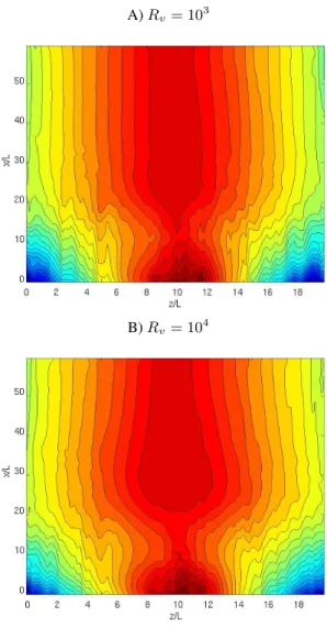
To investigate this point, Fig. 9 shows the magnetic sur-faces after the formation of a magnetic island above the cusp of the helmet streamer. As can be observed, indeed the
Fig. 8. History of the electric field energy for a run with the initial force-free reversed field equilibrium and withS=104andRv=104.
A)Rv= 10
3
B)Rv= 10
4
Fig. 9. Non-linear evolution of the initial 2-D helmet streamer equi-librium. Contours of the vector potentialAy, representing magnetic
surfaces, at timet /τA=200
process happens regardless of viscosity, and, as expected, the more viscous run shows a diminished speed of formation of the island. At a given same time in the two runs, the island is less developed in the higher viscosity case.
This conclusion is further confirmed by Fig. 10 that shows the evolution of the reconnected flux for the two runs with different viscosity (but equal resistivity). The reconnection process is similar but slightly faster for the lower viscosity run.
However, the fundamental difference of the 2-D equilib-rium when compared with the 1-D equilibequilib-rium of the previ-ous section is that also the acceleration of the blob is indepen-dent of viscosity. The mechanism allowing the acceleration is no longer the viscous drag exerted by the outer plasma on the forming island (augmented by the electric field) but rather is directly the converging flow at the cusp.
Fig. 10. Non-linear evolution of the initial 2-D helmet streamer equilibrium. Comparison of the time evolution for the reconnected flux in two runs with different viscosities (Rv=103andRv=104)
but equal resistivityS=104.
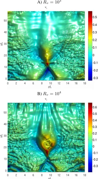
Figure 11 shows the vertical speed in the same two runs with different viscosity considered above. The flow velocity originating from the open field lines converges and focuses at the cusp in the region right below the forming island. The island finds itself in the same situation of a ball sitting atop a jet in a fountain: it is pushed by the jetting plasma. The converging flow focuses at the cusp and pushes the island upward by direct momentum transfer from the plasma to the island field lines. Viscous drag is no longer needed.
This last conclusion is demonstrated by Fig. 12 that shows the acceleration of the initially stagnant plasma above the cusp as a function of time. Clearly, viscosity is not the cause of the acceleration but rather just as it slows down by a small but perceptible amount the process of reconnection, it also slows down the ability of the converging flow to focus at the cusp and push the forming island upward.
6 Conclusions
A)Rv= 10
3
B)Rv= 10
4
Fig. 11. Non-linear evolution of the initial 2-D helmet streamer equilibrium. False colour representation of the vertical speed away from the Sunux (in the frame of reference of the Sun), at time t /τA=200. Two runs are shown with different viscosities (panel A: Rv=103and panel B:Rv=104) but equal resistivityS=104.
In the 1-D initial equilibrium, viscosity is shown to pro-vide the basic mechanism for momentum transfer from the slow solar wind to the forming blob. The viscous drag pro-duces a progressive acceleration of the plasma blob. The rate of increase of the slow solar wind speed (acceleration) is proportional to the viscosity in the simulation. However, an unexpected finding is that viscosity is not acting alone in its usual local drag action across layers of flowing plasma. Rather, the coupling between the accelerating island and the fast solar wind in the flanks is mediated by the global electric fields caused by the tearing instability forming the island. A
Fig. 12. Comparison of the time evolution of the vertical veloc-ity in the central axis in two runs starting from the initial 2-D hel-met streamer equilibrium with different viscosities (Rv=103 and Rv=104) but equal resistivityS=104.
direct numerical comparison of the evolution under pure vis-cous action and the full MHD evolution including the gener-ation of electromagnetic fields due to the tearing instability proves that the drag action is much increased from simple viscous drag.
In the 2-D initial configuration, the momentum transfer action is completely different. The viscous drag is not a de-termining factor in that it does not provide the mechanism for momentum transfer from the fast wind to the forming is-land. In the 2-D case, the flow merges at the cusp and simply pushes the island by direct momentum transfer acting in the same way a ball is pushed up by jetting water in a fountain. The momentum transfer in this case is coming directly by the action of plasma particles directed toward the magnetic filed lines of the island and being deflected by them. The change in momentum of deflected particles provides a direct accelerating force. Viscosity has no role to play and its effect is just to diminish the flows and to reduce the rate of island formation and its subsequent acceleration.
The results presented are relevant to the Sun where vis-cosity and resistivity due to direct collisional transport are extremely low. The ability to explain both in the 1-D and in the 2-D case how momentum transfer is provided by extra effects not directly due to viscosity is crucial. The results ob-tained here, as all other results obtainable within the range of currently achievable simulation cannot properly use the vis-cosity and resistivity of the real corona and cannot account self-consistently for anomalous processes. It is therefore cru-cial to show that the accelerating mechanisms presented here are indeed stronger than purely viscous processes would pro-duce and can sustain the scaling to realistic coronal parame-ters.
are not considered: the expanding geometry around the Sun (Rappazzo et al., 2005), the possible presence of Kelvin-Helmoltz instabilities driven in 3-D systems by differential foot-point motion (Lapenta and Knoll, 2003) and the expan-sion and acceleration of the solar wind away from the Sun. The role of gravity is also an important element in comput-ing correctly the blob acceleration. Future work will consider how the conclusions reached here are modified by these ad-ditional effects.
Acknowledgements. Fruitful discussions with R. Dahlburg and D. Knoll are gratefully acknowledged. The present work is sup-ported by the Onderzoekfonds K.U. Leuven (Research Fund KU Leuven), by the European Commission through the SOLAIRE net-work (MTRN-CT-2006-035484), by the NASA Sun Earth Connec-tion Theory Program and by the LDRD program at the Los Alamos National Laboratory. Work performed in part under the auspices of the National Nuclear Security Administration of the U.S. Depart-ment of Energy by the Los Alamos National Laboratory, operated by Los Alamos National Security LLC under contract DE-AC52-06NA25396. Simulations conducted in part on the HPC cluster VIC of the Katholieke Universiteit Leuven.
Topical Editor R. Forsyth thanks two anonymous referee for their help in evaluating this paper.
References
Barenblatt, G. I.: Scaling, Self-similarity, and Intermediate Asymp-totics, Cambridge University Press, Cambridge, 1996.
Bettarini, L., Landi, S., Rappazzo, F. A., Velli, M., and Opher, M.: Tearing and Kelvin-Helmholtz instabilities in the heliospheric plasma, Astron. Astrophys., 452, 321–330, 2006.
Biskamp, D.: Nonlinear Magnetohydrodynamics, Cambridge Uni-versity Press, Cambridge, UK, 1997.
Biskamp, D.: Magnetic Reconnection in Plasmas, Cambridge Uni-versity Press, Cambridge, UK, 2000.
Brackbill, J. U.: FLIP MHD – A particle-in-cell method for magne-tohydrodynamics, J. Comput. Phys., 96, 163–192, 1991. Braginskii, S. I.: Rev. Plasma Physics (I), p. 205, Consultants
Bu-reau Enterprises, New York, 1965.
Brueckner, G. E., Howard, R. A., Koomen, M. J., Korendyke, C. M., Michels, D. J., Moses, J. D., Socker, D. G., Dere, K. P., Lamy, P. L., Llebaria, A., Bout, M. V., Schwenn, R., Simnett, G. M., Bedford, D. K., and Eyles, C. J.: The Large Angle Spectroscopic Coronagraph (LASCO), Solar Phys., 162, 357–402, 1995. Daughton, W. and Karimabadi, H.: Kinetic theory of
collision-less tearing at the magnetopause, J. Geophys. Res., 110, 3217, doi:10.1029/2004JA010751, 2005.
Dorelli, J. C. and Birn, J.: Whistler-mediated magnetic recon-nection in large systems: Magnetic flux pileup and the for-mation of thin current sheets, J. Geophys. Res., 108, 1133, doi:10.1029/2001JA009180, 2003.
Einaudi, G., Bonicelli, P., Dahlburg, R., and Karpen, J.: Formation of the slow solar wind in a coronal streamer, J. Geophys. Res., 104, 521–534, 1999.
Einaudi, G., Chibbaro, S., Dahlburg, R. B., and Velli, M.: Plasmoid Formation and Acceleration in the Solar Streamer Belt, Astro-phys. J., 547, 1167–1177, 2001.
Endeve, E., Leer, E., and Holzer, T. E.: Two-dimensional Magneto-hydrodynamic Models of the Solar Corona: Mass Loss from the Streamer Belt, Astrophys. J., 589, 1040–1053, 2003.
Fisk, L. A. and Schwadron, N. A.: Origin of the Solar Wind: The-ory, Space Sci. Rev., 97, 21–33, 2001.
Goedbloed, J. P. H. and Poedts, S.: Principles of Magnetohydrody-namics, Cambridge University Press, Cambridge, 2004. Goossens, M.: An introduction to plasma astrophysics and
magne-tohydrodynamics, Kluwer, Dordrecht, The Nederlands, 2003. Knoll, D. A. and Chac´on, L.: Magnetic Reconnection in the
Two-Dimensional Kelvin-Helmholtz Instability, Phys. Rev. Lett., 88, 215003, 2002.
Landau, L. and Lifshitz, E.: Fluid Mechanics, vol. 6 of Course of Theoretical Physics, Pergamon, London, UK, 1959.
Lapenta, G. and Knoll, D. A.: Reconnection in the Solar Corona: Role of the Kelvin-Helmholtz Instability, Solar Phys., 214, 107– 129, 2003.
Lapenta, G. and Knoll, D. A.: Effect of a Converging Flow at the Streamer Cusp on the Genesis of the Slow Solar Wind, Astro-phys. J., 624, 1049–1056, 2005.
Mullan, D.: Source of the solar wind: What are the smallest-scale structures?, Astron. Astrophs., 232, 520–535, 1990.
Rappazzo, A. F., Velli, M., Einaudi, G., and Dahlburg, R. B.: Dia-magnetic and Expansion Effects on the Observable Properties of the Slow Solar Wind in a Coronal Streamer, Astrophys. J., 633, 474–488, 2005.
Schmidt, J. M. and Cargill, P. J.: A model for accelerated density enhancements emerging from coronal streamers in Large-Angle and Spectrometric Coronagraph observations, J. Geophys. Res., 105, 10 455–10 464, 2000.
Sheeley, Jr., N. R., Wang, Y.-M., Hawley, S. H., Brueckner, G. E., Dere, K. P., Howard, R. A., Koomen, M. J., Korendyke, C. M., Michels, D. J., Paswaters, S. E., Socker, D. G., St. Cyr, O. C., Wang, D., Lamy, P. L., Llebaria, A., Schwenn, R., Simnett, G. M., Plunkett, S., and Biesecker, D. A.: Measurements of Flow Speeds in the Corona between 2 and 30 R sub sun, Astrophys. J., 484, 472–478, 1997.
van Aalst, M. K., Martens, P. C. H., and Beli¨en, A. J. C.: Can Streamer Blobs Prevent the Buildup of the Interplanetary Mag-netic Field?, Astrophys. J. Lett., 511, L125–L128, 1999. Wang, Y.-M., Sheeley, Jr., N. R., Walters, J. H., Brueckner, G. E.,
Howard, R. A., Michels, D. J., Lamy, P. L., Schwenn, R., and Simnett, G. M.: Origin of Streamer Material in the Outer Corona, Astrophys. J. Lett., 498, L165, 1998.
Wiegelmann, T., Schindler, K., and Neukirch, T.: Helmet Stream-ers with Triple Structures: Weakly Two-Dimensional Stationary States, Solar Phys., 180, 439–460, 1998.
Wiegelmann, T., Schindler, K., and Neukirch, T.: Helmet Streamers with Triple Structures: Simulations of resistive dynamics, Solar Phys., 191, 391–407, 2000.