Modeling the present and future impact of aviation on climate: an AOGCM approach with online coupled chemistry

(1)

ACPD

13, 3817–3858, 2013

Modeling the climate impact of aviation

P. Huszar et al.

Title Page

Abstract Introduction

Conclusions References

Tables Figures

◭ ◮

Back Close

Full Screen / Esc

Printer-friendly Version Interactive Discussion

Discussion

P

a

per

|

Dis

cussion

P

a

per

|

Discussion

P

a

per

|

Discussio

n

P

a

per

Atmos. Chem. Phys. Discuss., 13, 3817–3858, 2013 www.atmos-chem-phys-discuss.net/13/3817/2013/ doi:10.5194/acpd-13-3817-2013

Atmospheric Chemistry and Physics

Open Access

Discussions

Geoscientiic Geoscientiic

This discussion paper is/has been under review for the journal Atmospheric Chemistry and Physics (ACP). Please refer to the corresponding final paper in ACP if available.

Modeling the present and future impact of

aviation on climate: an AOGCM approach

with online coupled chemistry

P. Huszar1,4, H. Teyss `edre1, D. Cariolle1,2, D. J. L. Olivi ´e1,3, M. Michou1, D. Saint-Martin1, S. Senesi1, A. Voldoire1, D. Salas1, A. Alias1, F. Karcher1,

P. Ricaud1, and T. Halenka4

1

GAME/CNRM, M ´et ´eo France, UMR3589, CNRS, Toulouse, France

2

Centre Europe ´en de Recherche et de Formation Avanc ´ee en Calcul Scientifique, CERFACS/CNRS, Toulouse, France

3

University of Oslo and CICERO, Oslo, Norway

4

Department of Meteorology and Environment Protection, Faculty of Mathematics and Physics, Charles University, Prague, V Hole˘sovi˘ck ´ach 2, Prague 8, 180 00, Czech Republic

Received: 11 January 2013 – Accepted: 1 February 2013 – Published: 11 February 2013

Correspondence to: P. Huszar ([email protected])

(2)

ACPD

13, 3817–3858, 2013

P. Huszar et al.

Title Page

Tables Figures

◭ ◮

Back Close

Full Screen / Esc

Discussion

P

a

per

|

Dis

cussion

P

a

per

|

Discussion

P

a

per

|

Discussio

n

P

a

per

|

Abstract

This work assesses the impact of emissions from global aviation on climate, while focus is given on the temperature response. Our work is among the first that use an Atmo-sphere Ocean General Circulation Model (AOGCM) online coupled with stratospheric chemistry and the chemistry of mid-troposphere relevant for aviation emissions. Com-5

pared to previous studies where either the chemical effects of aviation emissions were investigated using global chemistry transport models or the climate impact of aviation was under focus implementing prescribed perturbation fields or simplified chemistry schemes, our study uses emissions as inputs and provides the climate response as output. The model we use is the M ´et ´eo-France CNRM-CM5.1 earth system model ex-10

tended with the REPROBUS stratospheric scheme. The timehorizon of our interest is 1940–2100 assuming the A1B SRES scenario. We investigate the present and future impact of the most relevant aviation emissions (CO2, NOx, contrail and contrail induced cirrus – CIC) as well as the impact of the non-CO₂ emissions and the “Total” aviation impact. Aviation produced aerosol is not considered in the study.

15

The general conclusion is that the aviation emissions result in a less pronounced climate signal than previous studies suggest. Moreover this signal is more unique at higher altitudes (above the mid-troposphere) than near the surface.

The global averaged near surface CO2 impact reaches around 0.1◦C by the end of the 21st century and can be even negative in the middle of the century. The non-CO₂ 20

impact remains positive during the whole 21st century reaching 0.2◦_{C in its second} half. A similar warming is calculated for the CIC effect. The NOx emissions impact is almost negligible in our simulations, as the aviation induced ozone production was small in the model’s chemical scheme. As a consequence the non-CO2signal is very similar to the CIC signal. The seasonal analysis showed that the strongest warming 25

(3)

ACPD

13, 3817–3858, 2013

P. Huszar et al.

Title Page

Tables Figures

◭ ◮

Back Close

Full Screen / Esc

Discussion

P

a

per

|

Dis

cussion

P

a

per

|

Discussion

P

a

per

|

Discussio

n

P

a

per

the 21st century. A −0.3◦C temperature decrease is modeled when considering all the aviation emissions as well, but no significant signal is coming with CIC and NOx emissions in the stratosphere.

1 Introduction

The environmental stress of global aviation has been a concern since the 60s, early 5

70s (Osmundsen, 1963; Johnston, 1971; Johnston and Quitevis, 1971). Since these pioneering studies, large progress has been achieved in the understanding of aviation impact on the environment that resulted in two major assessments. The first one was undertaken by the Intergovernmental Panel for Climate Change (IPCC, 1999) and, re-cently, Lee et al. (2010) provided a comprehensive report on the issue. They accounted 10

for the impact of the emissions produced by aircraft on the atmospheric chemistry and climate only, however, aircraft produce significant noise, especially around airports, therefore the health e_ffects of aircraft noise is subject to investigation in many studies as well (e.g. Roselund et al., 2001).

Emissions of gases and aerosols from global aviation altering the chemical composi-15

tion of the atmosphere and, consequently, the change of abundances in the radiatively active gases and aerosols, have an impact on the radiative forcing (RF) and lead to temperature changes (Skeie et al., 2009). The condensation trail (contrail) formation from water vapor emissions and the induced cirrus cloud generate further RF from aviation.

20

The RF components from subsonic aviation originate from several processes (Lee et al., 2009). CO₂ (carbon dioxide) emissions increase the CO₂ levels and result in a positive RF. The range of 25.0–28.0 mW m−2_{was provided by the studies of Sausen} et al. (2005) and Lee et al. (2009) for the years 2000 and 2005. Emissions of NOx (nitrogen oxides) trigger through a chain of chemical reactions the formation of O₃ 25

(4)

ACPD

13, 3817–3858, 2013

P. Huszar et al.

Title Page

Tables Figures

◭ ◮

Back Close

Full Screen / Esc

Discussion

P

a

per

|

Dis

cussion

P

a

per

|

Discussion

P

a

per

|

Discussio

n

P

a

per

|

reduction that represents a negative RF (Stevenson et al., 2004). Finally, a long-term small O3 decrease is attributed to this methane reduction resulting in a negative RF (K ¨ohler et al., 2008). The RF estimates of the latter study for these three components are of 30 mW m−2_,

−19 mW m−2and−11 mW m−2, respectively for the 2002 emissions. This gives a zero net forcing. Stevenson et al. (2004) reached the same conclusion 5

indicating an overall low RF due to aviation NOx emissions.

Aircraft emit water vapor (H₂O) that is a greenhouse gas with a positive RF estimated to 2.8 mW m−2_{by Lee et al. (2009) for 2005. The most recent study, Wilcox et al. (2012)} however updates H2O vapor RF to a smaller value of 0.9 mW m−

2 .

An important effect of aircraft H2O emissions routinely observed is the formation of 10

persistent contrails and contrail cirrus (Atlas et al., 2006). Contrails are line-shaped cir-rus that form after the mixing of the hot and moist air from the aircraft engines with the ambient air while the Schmidt-Appelman criterion (Schumann, 1996) has to be fulfilled requiring the air being under a critical temperature. According to the local meteorolog-ical conditions, a contrail can undergo shear, uplift and mixing that results in its areal 15

extent – a contrail cirrus is formed. The contrail ice nuclei can also modify the natural cirrus cloudiness (Boucher, 1999). Hereafter, we will use the term “Contrail Induced Cloudiness” (CIC) that will refer to contrails, contrail cirrus and natural cirrus modifica-tions mentioned later. We have to point out that the term “Aviation Induced Cloudiness” (AIC) is defined as well (Lee et al., 2010) that adds aircraft soot generated cloudiness 20

to CIC.

The detection (measurement), properties, formation, evolution and radiative effects of CIC have been subject to a large number of studies (Zerefos et al., 2003; Schumann, 2005; Stordal et al., 2005; Gao et al., 2006; Hong et al., 2008; Fr ¨omming et al., 2011). The physical mechanism behind its formation is now well understood but due to the 25

(5)

ACPD

13, 3817–3858, 2013

P. Huszar et al.

Title Page

Tables Figures

◭ ◮

Back Close

Full Screen / Esc

Discussion

P

a

per

|

Dis

cussion

P

a

per

|

Discussion

P

a

per

|

Discussio

n

P

a

per

for the year 2005 (Lee et al., 2009). The most up-to-date CIC RF estimate is given by Burkhardt and K ¨archer (2011), 31 mW m−2_{for year 2005.}

Aircraft black carbon (BC) emissions represent a tiny fraction of the total emitted anthropogenic BC mass, but BC particles originating from aircraft engines are much smaller than from other sources. Thus the number concentration of BC is perturbed sig-5

nificantly due to aviation (Hendricks et al., 2004). RF estimates for BC recently given by Balkanski et al. (2010), are of 0.1 or 0.3 mW m−2_{depending on whether BC externally} or internally mixed with sulphate is considered. In contrast, a one order larger negative RF is calculated by the same authors for aviation sulphate aerosols (∼1 mW m−2).

The total RF of aviation was evaluated by Sausen et al. (2005) for 2000, and recently 10

by Lee et al. (2010) for 2005, giving positive RF of 47.8 mW m−2 _{and 55.0 mW m}−2_, respectively. These values included linear contrails (around 10 mW m−2_{) but excluded} the aviation induced cirrus cloudiness that is very uncertain in terms of its related RF. The latter can be however estimated from the latest CIC estimate from Burkhardt and K ¨archer (2011) to be of 21 mW m−2_{. So the total RF from the aviation sector for the} 15

year 2005 is around 70–75 mW m−2_.

The above positive RF represents a considerable contribution to the total anthro-pogenic RF of 1660 mW m−2_{(Lee et al., 2010) and it may be responsible for significant} warming and other changes (e.g. precipitation). Furthermore, this forcing is expected to gradually increase towards the end of the 21th century (Skeie et al., 2009) therefore 20

its impact might rise as well. The response of the climate system to a given radiative forcing is delayed due to its thermal inertia (Hansen et al., 2005). If the land-surface and the ocean mixed layer are only considered, the timescale of the response is of 1 to 5 yr (Olivi ´e and Stuber, 2010). Taking into account the deep ocean response, this timescale changes to several centuries. In terms of intensity, the fast response con-25

(6)

ACPD

13, 3817–3858, 2013

P. Huszar et al.

Title Page

Tables Figures

◭ ◮

Back Close

Full Screen / Esc

Discussion

P

a

per

|

Dis

cussion

P

a

per

|

Discussion

P

a

per

|

Discussio

n

P

a

per

|

simplified model approaches that cannot give answer about the geographic distribution of the impacts.

To investigate the long term response of a varying anthropogenic forcing (such as aviation), including its geographic and vertical distributions, a more sophisticated ap-proach, the use of an AOGCM (AtmospheOcean General Circulation Model) is re-5

quired as it describes the atmosphere, ocean and sea-ice and the interactions between them in detail. This is certainly a computationally demanding task and for the aviation impact, Olivi ´e et al. (2012) is one of the few studies that adopted this approach. They assessed the climate impact of all transport sectors (road, shipping and aviation) for the period 1860–2100. The AOGCM they applied did not contain detailed chemistry of 10

the atmosphere but a simplified O₃scheme (Cariolle and Teyss `edre, 2007). Therefore the forcing agents (like CO2, aerosols etc.) perturbed by the specific transport sector were provided externally as global constants or 3-D fields. For ozone, two approaches were adopted: in the first one, they prescribed 3-D perturbed ozone fields, in the sec-ond one, the simplified ozone scheme was used. The CIC were not calculated online 15

during the simulations, but an external data source served to track its presence in the model atmosphere and was later provided to the radiative code of the AOGCM.

Here we present a novel approach to evaluate the climate-chemistry impact of avi-ation emissions: we use a similar AOGCM to that of Olivi ´e et al. (2012), the novelty being that, in our AOGCM, we consider online coupled chemistry limited to the mid-20

troposphere and stratosphere, regions that encompass the altitudes where the air-traffic and their emissions mostly occur. This allows us to use the aviation emissions as inputs to the model (i.e. not the concentration perturbations) and to account for all the chemical processes triggered by these emissions. Our main focus in this paper will be the 3-D temperature response to these aviation emissions, investigating the 25

1940–2100 period.

(7)

ACPD

13, 3817–3858, 2013

P. Huszar et al.

Title Page

Tables Figures

◭ ◮

Back Close

Full Screen / Esc

Discussion

P

a

per

|

Dis

cussion

P

a

per

|

Discussion

P

a

per

|

Discussio

n

P

a

per

radiative impact negligible as confirmed recently by Wilcox et al. (2012). Previous stud-ies showed (see above) that aerosol originating from the aviation sector has a minor climate impact, so in our study aviation related aerosols (soot and sulphates) will not be considered. As in many transport related impact studies, we will distinguish between CO₂and non-CO₂impacts that represent the climate impact of the CO₂emissions only 5

and that of all other emissions. Further we present the NOx impact, i.e. the impact of the NOx emissions only, and the CIC impact, i.e. the impact of the contrails and the induced cirrus alone. Finally, the total aviation impact will be evaluated as well.

2 Tools and experimental set-up

2.1 Model CNRM-CM

10

In our work, we used the atmospheric-chemistry model coupled with an ocean/sea ice model, denoted as CNRM-CCM model hereafter. It is an extension of the Ocean/Atmosphere General Circulation Model CNRM-CM5.1 that is extensively de-scribed in Voldoire et al. (2012).

In summary, CNRM-CM is a state-of-the-art general circulation model that has been 15

jointly developed by CNRM-GAME (Centre National de Recherches M ét éorologiques – Groupe d’ études de l’Atmosph ère M ét éorologique) and CERFACS (Centre Europ éen de Recherche et de Formation Avanc ée) in order to contribute to phase 5 of the Coupled Model Intercomparison Project (CMIP5, see http://cmip-pcmdi.llnl.gov/cmip5/ experiment design.html). CNRM-CM5.1 includes the atmospheric model ARPEGE-20

Climat (v5.2), the ocean model NEMO (v3.2; Madec, 2008), the land surface scheme ISBA and the sea ice model GELATO (v5; Salas, 2002) coupled through the OASIS (v3; Valcke, 2006) system. Horizontal resolution of the atmosphere is about 1.4◦_{and 1}◦ _for the ocean. The atmospheric component uses the Morcrette et al. (2001) scheme over 6 bands for the solar radiation and the RRTM scheme for the long-wave radiation. Seven 25

(8)

ACPD

13, 3817–3858, 2013

P. Huszar et al.

Title Page

Tables Figures

◭ ◮

Back Close

Full Screen / Esc

Discussion

P

a

per

|

Dis

cussion

P

a

per

|

Discussion

P

a

per

|

Discussio

n

P

a

per

|

O₃is a prognostic variable with photochemical production and loss rates computed off -line by a 2-D zonal chemistry model (MOBIDIC; Cariolle and Teyss `edre, 2007). H2O is a prognostic variable and the other 5 absorbents are prescribed to a uniform value that evolves on a yearly basis. The climatology of tropospheric aerosols from Szopa et al. (2012) is prescribed, while the land surface scheme has been externalised from 5

the atmospheric model through the SURFEX platform. It includes new developments such as a parameterization of sub-grid hydrology, a new soil freezing scheme and the ECUME bulk parameterization for ocean surface fluxes.

2.2 CNRM-CM chemistry version: CNRM-CCM

The atmospheric model embedded in CNRM-CCM is the one used for CNRM-CM5, 10

described in the previous paragraph. The main difference resides in the “online” cou-pling with a stratospheric chemistry which is based on the REPROBUS stratospheric chemistry scheme (Lef `evre et al., 1994). This chemistry is applied on the whole vertical column, except between the surface and the 700 hPa level where long-lived chemical species are relaxed towards global average surface value following the A1B scenario. 15

Convection of species is not considered. In this chemistry version, the 3-D distribution of the seven absorbing gases is then provided by the chemistry module of CNRM-CCM and interacts with the radiative calculations. More details can be found in Michou et al. (2011).

In the CNRM-CM default version, there are only 31 vertical levels of which 5 are in 20

the stratosphere. For stratospheric chemistry studies, the number of vertical levels has been increased to 60 layers (26 of them being in the stratosphere). This increase of vertical resolution requires to reduce the time-step from 30 to 15 min. Additionally, as there are about 50 3-D supplementary species, the horizontal resolution was reduced from 1.4◦_{to 2.8}◦_{to reduce computational costs. As a consequence of the resolution} de-25

(9)

ACPD

13, 3817–3858, 2013

P. Huszar et al.

Title Page

Tables Figures

◭ ◮

Back Close

Full Screen / Esc

Discussion

P

a

per

|

Dis

cussion

P

a

per

|

Discussion

P

a

per

|

Discussio

n

P

a

per

paragraphs. Finally, this version of CNRM-CCM costs about 21 h of elapsed-time to simulate one year on the NEC supercomputers of M ´et ´eo-France.

2.3 Emission data

The emission data we used were developed within the QUANTIFY project, an Inte-grated Project funded through the EU-Framework Programme 6 (Lee et al., 2005)(see 5

http://www.ip-quantify.eu). For aviation, they consist in 3-D data with a horizontal reso-lution of 1◦

×1◦. and a 610 m vertical spacing up to 14 km.

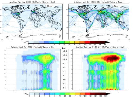
These data contain monthly totals of fuel consumption and emissions for NOx and soot as kg gridbox−1_month−1_{. They are only available for years 2000, 2025, 2050, and} 2100 (see Fig. 1 for the 2000 and 2100 horizontal and zonally averaged fuel consump-10

tion distribution). For the period 1940–2100, time series of global emission estimates are also included (see Fig. 2). In 1940, the emissions are identically zero, since this year is considered as the beginning of significant aviation activities (Sausen and Schu-mann, 2000). Until 2020, FESG forecast values are adopted (FESG, 2008), which as-sumes that the fuel efficiency continues with recent trends and that NO_ximprovements 15

commensurate with insertion of the best of present-day technology. The QUANTIFY dataset does not contain explicitly military aviation emissions, however the civil avia-tion emission patterns are scaled to the IEA aviaavia-tion fuel-burn totals.

To provide 3-D emission data for other years than those available in the emission inventory (i.e. for the whole period 1940–2100), we linearly interpolated the emissions 20

in time and normalized them with their annual totals.

When assessing the role of the NOx aviation emissions, the lightning NOx (LNOx) has to be taken into account since several studies (Bernsten et al., 1999; Grewe, 2003; Schumann and Huntrieser, 2007) have shown that it is another major source of NO_x in the atmosphere. This has important implications for the atmospheric chemistry and 25

(10)

ACPD

13, 3817–3858, 2013

P. Huszar et al.

Title Page

Tables Figures

◭ ◮

Back Close

Full Screen / Esc

Discussion

P

a

per

|

Dis

cussion

P

a

per

|

Discussion

P

a

per

|

Discussio

n

P

a

per

|

taken from the ANCAT lightning NO_xemission monthly climatology defined for the year 1992. For other years, we applied a scaling on the global mean surface temperature as suggested by Schumann and Huntrieser (2007) who estimate a 10% increase of lightning activity and emitted LNO_x by each 1 K of global mean surface temperature increase.

5

Emissions from aviation and lightning had to be implemented into CNRM-OACCM that originally did consider neither 2-D nor 3-D emissions. They are read in by the model at the beginning of each simulated month, interpolated to the model grid and converted to emissions densities that the model uses in the continuity equations to calculate the temporal evolution of the chemical species. We also adopted the temporal 10

disaggregation of the monthly emission values given by Wilkerson et al. (2010). They provide weekly and hourly global profiles, so profiles are the same for every geographic region and reflect the evolution of the global emission value and not the actual local variation of the emissions.

2.4 Parameterizations

15

The small-scale processes during the dilution of the aircraft emission plume cannot be explicitly resolved in our experimental set-up due to our coarse model resolution. How-ever, these processes can imply changes at the model resolved scale, e.g. can lead to modified chemical species concentrations and/or can consequently have radiative impacts.

20

One of these subgrid scale processes is the chemical evolution of the NO_xemissions in the aircraft engine plume and the subsequent ozone formation. It was shown by many authors (e.g. Kraabøl et al., 2002; Cariolle et al., 2009, and references therein) that disregarding the chemical non-linearities in the NO_x-plumes behind the aircraft by applying instantaneous dilution at the model scale (as it is usually done in chemistry 25

(11)

ACPD

13, 3817–3858, 2013

P. Huszar et al.

Title Page

Tables Figures

◭ ◮

Back Close

Full Screen / Esc

Discussion

P

a

per

|

Dis

cussion

P

a

per

|

Discussion

P

a

per

|

Discussio

n

P

a

per

well (Huszar et al., 2010), introduces a “fuel” tracer with a certain lifetime that traces the amount of material in the plume. The large scale NO_xand O₃concentrations are then modified according to the concentration of this tracer using an effective reaction rate for the ozone formation. The method of Cariolle et al. (2009) has been implemented into CNRM-CCM.

5

Another aspect of the subgrid scale processes occurring in the aircraft plume is the condensation of water vapor emitted, and the subsequent formation of contrails and contrail cirrus (depending on the meteorological conditions). We have not considered a parameterization of the formation and evolution of the contrails, however as the ra-diative effects of the CIC are of great importance and cannot be neglected, we have 10

developed a simplified treatment of these processes and their related radiative e_ffects. Our method, similar to that of Olivi ´e et al. (2012) is summarized below.

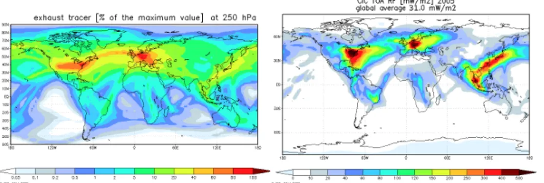
First we introduce a contrail tracer (in a similar way as the “fuel” tracer mentioned above) with a certain lifetime (15 h). The modeled distribution of this tracer on the 250 hPa level, representing the main flight level, is plotted in Fig. 3 (left). CIC is ex-15

pected to form where temperature is less than −40◦C and the relative humidity ex-ceeds 80 %. In model grid points fulfilling these conditions, we add the contrail tracer concentration, multiplied by a given factor, to the large scale cloud ice mixing ratio. The value of this multiplicative factor is tuned to obtain an appropriate annual global value of the top-of-the-atmosphere radiative forcing for the contrail and contrail induced cirrus 20

for 2005. This target value is taken from Burkhardt and K ¨archer (2011), 31 mW m−2_, representing the most recent estimate. This factor is held constant between 1940 and 2100. The distribution of the TOA radiative forcing due to CIC for the year 2005 is seen in Fig. 3.

As pointed out in the model description, the chemistry is resolved in the strato-25

(12)

ACPD

13, 3817–3858, 2013

P. Huszar et al.

Title Page

Tables Figures

◭ ◮

Back Close

Full Screen / Esc

Discussion

P

a

per

|

Dis

cussion

P

a

per

|

Discussion

P

a

per

|

Discussio

n

P

a

per

|

further below), these lower boundary conditions have to reflect the situation that would occur if the whole troposphere was treated by explicit chemistry. In the case of CO₂, an increase occurs due to aircraft emissions, while in the case of methane, aircraft NOx enhance OH concentrations which accelerate methane reduction through a chemical reaction with OH. Therefore we have prescribed the aviation CO₂ contribution and 5

methane reduction in the tropospheric relaxation values.

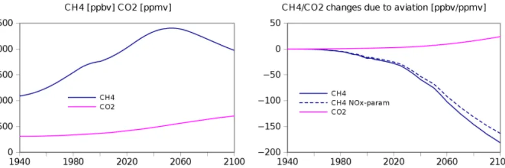
For CO2, Skeie et al. (2009), who uses the same emission inventory as in this study, provide the aviation CO₂contribution until the end of the 21th century. The evolution of this contribution in ppmv is plotted in Fig. 4 (right, pink line).

The magnitude of the methane reduction due to aviation NOx emissions has been 10

calculated following Olivi ´e et al. (2012). They used the hydroxyl radical perturbation due to aviation for present as well as for 2025 and 2050 conditions in 3 different CTMs (Hodnebrog et al., 2011) to calculate the methane lifetime reduction and its consequent reduction of concentration. For intermediate years from 1940 to 2100 we inter- and extrapolated the OH enhancement and therefore the methane changes.

15

We have to point out that these results did not consider the in-plume chemical non-linearities that we have mentioned earlier and which result in a lower OH enhancement and subsequently in a smaller methane reduction. Kraabøl et al. (2002) calculated that the change of the methane lifetime becomes∼9 % smaller when plume processes are considered. We used this correction in our methane lifetime reduction. The 1940–2100 20

evolution of the CO2and methane absolute concentrations as well as of the perturba-tions due to the aviation NOxemissions with/without the NOx-plume parameterization, for the A1B scenario, can be seen in Fig. 4 (right, blue line).

2.5 Model simulations

The goal of the study is to evaluate the aviation impact on chemistry and climate for the 25

(13)

ACPD

13, 3817–3858, 2013

P. Huszar et al.

Title Page

Tables Figures

◭ ◮

Back Close

Full Screen / Esc

Discussion

P

a

per

|

Dis

cussion

P

a

per

|

Discussion

P

a

per

|

Discussio

n

P

a

per

for the year 1940, both for the atmospheric part of the model including its chemical composition as well as for the ocean and the sea ice.

Another task before starting the “impact-simulations”, i.e. the experiments over the period 1940–2100 considering the aviation emissions, is to ensure that the chosen model configuration is able to simulate the climate system reasonably without signifi-5

cant biases and trends when the forcings are set constant.

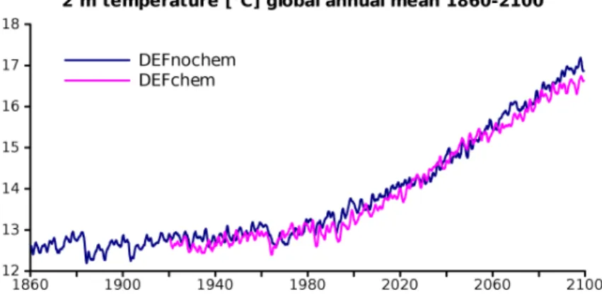
To meet these requirements, a 100-yr spinup was integrated under the 1860 condi-tions (i.e. greenhouse gas concentracondi-tions – GHG and solar constant). In this spinup, the online chemistry was turned off. After this spinup, the model was run further to-wards the end of the 21st century with forcings according to the A1B scenario. This 10

experiment is denoted DEFnochem, as this simulation applied the default model that used standard GHG evolutions while no 3-D aviation emissions were explicitly sup-plied, which however means that the aviation impact was included implicitly through the prescribed GHG concentrations.

A simulation called DEFchem in which the chemistry scheme is activated has been 15

started from year 1920 of DEFnochem. Years 1920–1940 are then considered as spin-up years to allow the chemical composition of the atmosphere to be in equilibrium with the mean climate of the model. We have checked that 20 yr is enough to initialize the chemistry in order to have consistent initial conditions for 1940.

For the period 1940–2100 we performed several experiments with aviation forcings 20

(CO2, NOx, CIC) turned off/on (i.e. whether the related emissions or the contrails are considered or not). These (as well as the default simulations) are summarized in Ta-ble 1.

All the effects are accounted for in the experiment denoted “ALL”. In the noCIC ex-periment, the effect of contrails and contrail induced cirrus is removed. In the “noCI-25

(14)

ACPD

13, 3817–3858, 2013

P. Huszar et al.

Title Page

Tables Figures

◭ ◮

Back Close

Full Screen / Esc

Discussion

P

a

per

|

Dis

cussion

P

a

per

|

Discussion

P

a

per

|

Discussio

n

P

a

per

|

In order to identify the climate signal caused by these effects, we have to account for the e_ffect of the variability of the modeled climate. We achieved this by performing ensembles of 3 members for all “impact simulations” (1–5 in Table 1). A larger ensem-ble was impossiensem-ble due to the computational costs of the experiments due to online coupled chemistry. These ensembles were performed over the 2000–2100 period, as 5

we expect negligible impact of aviation for the 1940–1999 period following Olivi ´e et al. (2012). The year 2000 perturbation required for the 2nd and the 3rd members of the mini-ensemble was obtained by restarting from 1 January 1999 and 2001 instead of 2000 as done in the 1st (original) member. Hereafter, results shown for the 2000–2100 period will by default represent ensemble means from these three simulations, unless 10

explicitly stated otherwise.

The impact of an individual emission or all aviation emissions has been evaluated as a difference of appropriate experiments, in particular:

– CO₂-impact: noCIC experiment – noCICnoCO2 experiment

– NOx-impact: noCIC experiment – noCICnoNOx experiment 15

– CIC impact: ALL experiment – noCIC experiment

– non-CO2-impact: ALL experiment – noCICnoNOx experiment

– Total impact: ALL experiment – noAVIATION experiment

3 Results

3.1 Overall climate change since the preindustrial times

20

(15)

ACPD

13, 3817–3858, 2013

P. Huszar et al.

Title Page

Tables Figures

◭ ◮

Back Close

Full Screen / Esc

Discussion

P

a

per

|

Dis

cussion

P

a

per

|

Discussion

P

a

per

|

Discussio

n

P

a

per

chemistry with respect to 1860 is about 1.0, 2.5 and 4.5◦_{C for the years 2000, 2050 and} 2100, respectively. This holds for the warming simulated by the DEFchem experiment as well, although by the end of the century this warming tends to be less than that of the experiment without online coupled chemistry (DEFnochem) by around 0.3–0.5◦_C.

In the DEFnochem simulation, the Arctic sea-ice extent is generally over-estimated, 5

especially over the Northern Atlantic. We attributed this bias to the large difference between the resolution of the atmospheric model (2.8◦

×2.8◦) and that of the sea ice model (1◦

×1◦). To prove this affirmation we performed a sensitivity run with 1.4◦×1.4◦ resolution for the atmospheric model and we found that this run does not exhibit this sea ice bias over the Arctics. As the atmospheric model calculates mean fluxes over 10

grid boxes that may be only partially covered with sea-ice, this may not be appropriate for the grid cells of the sea ice model. This high sea-ice extent bias persisted in the model simulations throughout the 20th and 21st centuries.

3.2 The mean global impact of different aviation emissions

In this section we present the global mean temperature response due to different avi-15

ation emissions as the difference in the corresponding experiments (see previous sec-tion). Figure 6 shows these di_fferences in the corresponding ensemble members (thin lines) and in the 11-yr running mean of the ensemble means (thick lines) for the tem-perature at the surface (2 m) and at selected pressure levels, i.e. 850, 500, 250, 100 and 10 hPa, between 2000 and 2100.

20

Aviation emissions represent a positive RF causing warming in the troposphere. In the 20th century this effect is considered rather negligible but, with increasing emis-sions and related RF, it is expected to reach significant levels towards the end of the 21th century (Skeie et al., 2009; Olivi ´e et al., 2012). As seen in Fig. 6, in our simula-tions the modeled impact on the 11-yr running mean temperature exhibits large vari-25

(16)

ACPD

13, 3817–3858, 2013

P. Huszar et al.

Title Page

Tables Figures

◭ ◮

Back Close

Full Screen / Esc

Discussion

P

a

per

|

Dis

cussion

P

a

per

|

Discussion

P

a

per

|

Discussio

n

P

a

per

|

However, the variability in the temperature response is still very large, especially for the 2 m temperature.

In general, the increase of temperature due to aviation emissions is visible when considering the CIC effect, the non-CO2 effect and all aviation related emissions (the “Total” impact). The temperature response is evident especially at higher levels of the 5

troposphere, i.e. at 500 and 250 hPa. A warming of up to 0.1◦_{C is predicted for the} last two decades of the 21st century due to CIC impact (blue line) or non-CO2impact (brown line).

The expected warming due to aviation CO2 is visible only at the end of the 21st century, reaching about 0.1◦_{C at the surface and at higher levels in the troposphere.} 10

However, in the upper stratosphere (at 10 hPa), CO₂ emissions from aviation lead to significant cooling that reaches−0.25◦C.

Our modeling system does not simulate a significant change of global mean temper-ature due to aviation NO_x emissions. In the next section we show that this is probably connected to limiting the chemistry to the upper troposphere and the stratosphere and 15

the fact that the tropospheric species, including methane, were prescribed. This im-posed a large negative forcing due to methane reduction and, with the reduced ozone production, leaded to small radiative forcing due to aviation NOx emissions and thus negligible temperature response. As a consequence, the non-CO2impact goes in line with the CIC impact reflecting that its major component – the NO_xemission impact – is 20

small in our simulations.

Finally, the largest temperature response is simulated when considering all the avi-ation emissions (green line), up to a 0.2◦_{C warming at higher levels in the mid} tropo-sphere towards the end of the century, with a warming present during the entire period. Above the main flight levels, aviation emissions cause a slight cooling at 100 hPa 25

(17)

ACPD

13, 3817–3858, 2013

P. Huszar et al.

Title Page

Tables Figures

◭ ◮

Back Close

Full Screen / Esc

Discussion

P

a

per

|

Dis

cussion

P

a

per

|

Discussion

P

a

per

|

Discussio

n

P

a

per

3.3 The three-dimensional structure of the aviation impact on the temperature

of the atmosphere

The globally averaged impact of aviation does not provide a detailed picture of the spatial distribution of its magnitude and of the statistical significance of the changes. Here we choose three 20-yr periods: 1991–2010, 2031–2050 and 2080–2099 repre-5

senting the present-day, near future and far future conditions. We examine the change of temperature averaged over these 20 yr due to aviation emissions. The analysis is performed for the near surface temperature and for the zonal means. In order to draw a picture of the seasonality of the impacts, we calculate the monthly variation of the temperature changes as well.

10

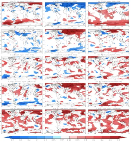
3.3.1 Spatial patterns of the near surface temperature changes

In Fig. 7, the change in the global near surface temperature due to different aviation emissions is presented for the three periods, corresponding to the three columns from left to right.

The figure shows that the CO2-impact (first row) is very small in the present day 15

decades with small areas of statistically significant changes. It becomes stronger in the near future resulting in a decrease in temperature. The strongest impact is simulated during the far future period: statistically significant warming occurs over large areas at low latitudes and the Antarctic (up to 0.2◦_{C), with an even higher warming around the} South Pole, up to 0.4◦_{C. Cooling is limited to the Arctics.}

20

The impact of aviation NOxemissions (second row) on near surface temperature is small in general and statistically significant over small areas with both warmings and coolings, in the−0.3–0.3◦C range. The largest temperature changes (warmings) are modeled over the Arctic, especially in the near future.

The CIC impact of on the near surface temperature suggests warming, although it 25

(18)

ACPD

13, 3817–3858, 2013

P. Huszar et al.

Title Page

Tables Figures

◭ ◮

Back Close

Full Screen / Esc

Discussion

P

a

per

|

Dis

cussion

P

a

per

|

Discussion

P

a

per

|

Discussio

n

P

a

per

|

The non-CO₂impact (Fig. 7, fourth row) resembles the CIC effect, reflecting the low NOx-impact modeled in our study. This impact is however stronger than the CIC one, with warming often exceeding 0.6◦_{C over the Arctic. Over other regions, the non-CO}

2 emissions are responsible for a warming around 0.1–0.2◦_{C in the far future, although} the areas with significant changes are limited.

5

More significant impacts are obtained when considering the combined effects of the emissions (Fig. 7, bottom row). The warming near the surface is significant during each examined time-slice. It can be as high as 0.6◦_{C over some regions in each period, but} the area of statistical significance increases towards the end of the century.

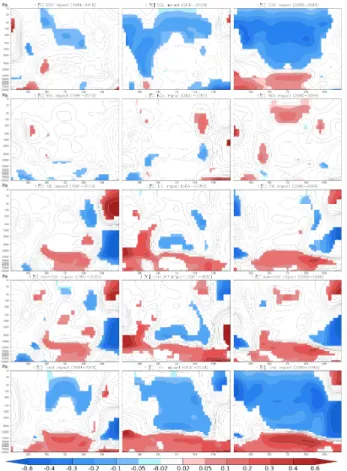
3.3.2 Zonal mean temperature changes due to aviation emissions

10

This section provides results on the zonally averaged temperature response over the three periods analyzed in the previous section. The results are presented in Fig. 8 where each row corresponds again to a particular emissions or their combinations (from top to bottom: CO₂, NO_x, CIC, non-CO₂ and Total impact). The figure suggests that aviation emissions are, in general, responsible for warming in the troposphere and 15

cooling in the stratosphere. The main cause of the stratospheric cooling are the CO2 emissions, and this is why this cooling is well expressed in the “Total” impact as well. It remains negligible in present day conditions, reaches−0.1 to−0.2◦C in the middle of the century, and becomes the strongest towards the end of the century (−0.3 to −0.4◦C). Taking into account all the aviation emissions, the stratospheric cooling is 20

even more pronounced, reaching−0.6◦C in zonal average in the far future.

Statistically significant zonally averaged tropospheric warming is computed for the CO2-impact only in 2080–2099, from 90◦S to 40◦N. This warming reaches 0.1◦C over the equatorial belt and becomes even stronger over the Antarctic.

The zonal temperature changes due to NOxemissions are not significant, except for 25

a warming over the Equator in the upper stratosphere (around 20–100 Pa).

(19)

ACPD

13, 3817–3858, 2013

P. Huszar et al.

Title Page

Tables Figures

◭ ◮

Back Close

Full Screen / Esc

Discussion

P

a

per

|

Dis

cussion

P

a

per

|

Discussion

P

a

per

|

Discussio

n

P

a

per

this warming becomes larger and significant at almost all latitudes, with higher values over the Northern Hemisphere (up to 0.3◦_{C). In the far future, the temperature increase} due to CIC is well emphasized between 60◦_{S and 60}◦_{N, encountering maxima (of 0.3–} 0.4◦_{C) over 40–50}◦_{N corresponding to the denser aviation routes (see Fig. 3).}

The aviation non-CO₂emission induced temperature changes are again very similar 5

to the CIC impact in magnitude. Highest values of warming in the troposphere are modeled over the Northern Hemisphere with maxima over the Arctic in the near future, and around the main flight corridors in the far future where temperature increases up to 0.3–0.4◦_C.

Apart from the well expressed decrease in the stratosphere, an intensive tempera-10

ture increase due to all aviation emissions is encountered in the troposphere in each period. In near and far future it covers almost all latitudes, and it reaches maximal values over the Northern Hemisphere (0.4–0.6◦_{C) in the far future.}

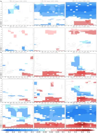
3.3.3 Seasonal dependence of the aviation impacts on temperature

Aviation emissions are not uniformly distributed along the year but show a monthly vari-15

ation peaking in July-August and being lowest in January (Olsen et al., 2013) and this seasonal variation is represented in the emission data we use as well. Furthermore, the environmental conditions under which these emissions trigger further e_ffects, like tem-perature, prevailing winds, humidity etc. vary by season as well. Therefore, we might also expect a seasonal dependence of the impacts of the aviation emissions as well. 20

To evaluate this dependence, we plotted the change of the monthly variation of tem-perature (see Fig. 9) providing information about the seasonal variation of the impact at all altitudes.

The main features of the impacts seen in the previous paragraphs appear also in Fig. 9, i.e. (1) during 1991–2010 the low, statistically not significant impact for the CO2 25

(20)

ACPD

13, 3817–3858, 2013

P. Huszar et al.

Title Page

Tables Figures

◭ ◮

Back Close

Full Screen / Esc

Discussion

P

a

per

|

Dis

cussion

P

a

per

|

Discussion

P

a

per

|

Discussio

n

P

a

per

|

Figure 9 further shows that the CO₂ tropospheric impact is significant during late spring until autumn with a maximum around September. The CO2induced cooling in the stratosphere is significant in both the near and far future in all seasons.

For the NO_x impact, only a small area of significant warming in the stratosphere above 100 Pa is simulated, throughout most of the year.

5

The CIC impact is the largest during early autumn in the present day period and is increasing in the middle and far future, with a shift of the maximum values to June and July. A small but statistically significant temperature decrease during late spring and early summer appears in the stratosphere.

The seasonal dependence of the non-CO₂ impact is similar to the CIC impact with 10

a maximum tropospheric warming in September, a second local maximum for the near future in June and a stronger warming in 2080–2099 peaking in the summer months. The stratospheric cooling is present as well.

The impact of all the emissions (total impact) is significant in every season, in both the troposphere and the stratosphere and practically in each examined period. The 15

largest tropospheric warming occurs during October 1991–2010 and during the sum-mer in the two future periods.

3.4 Impact on atmospheric chemistry

This section presents the changes in the amount and 3-dimensional distribution of relevant air pollutants due to aviation emissions. Focus is given to the CO2 and NOx 20

emissions and the triggered ozone change.

Previous studies dealing with the aviation CO2impact considered it as uniformly dis-tributed over the globe (e.g. Olivi ´e et al., 2012) given its long lifetime. However, to some extent the aviation contribution to the CO₂distribution is not uniform and its maximum is concentrated in the Northern Hemisphere. Figure 10 presents the zonally averaged 25

(21)

ACPD

13, 3817–3858, 2013

P. Huszar et al.

Title Page

Tables Figures

◭ ◮

Back Close

Full Screen / Esc

Discussion

P

a

per

|

Dis

cussion

P

a

per

|

Discussion

P

a

per

|

Discussio

n

P

a

per

periods. In the troposphere, the contribution goes down to 1.4, 5.3 and 19.5 ppmv, while in the stratosphere it decreases to 1.1, 4.6 and 17.8 ppmv, respectively.

The zonally averaged impact of aircraft NOx emissions on the NOx and ozone con-centrations is presented in Fig. 11. For NOx, significant changes occur at the main flight levels over the Northern Hemisphere, becoming important in the Southern Hemisphere 5

as well in 2080–2099. The contribution reaches 50, 100 and 150 pptv for the three pe-riods, respectively. Regions of significant changes occur in the stratosphere as well, with a decrease up to−30 pptv in the near future and an increase over 100 pptv in the far future.

The aviation induced, zonally averaged ozone changes (Fig. 11, bottom row) are 10

very small in the 1991–2010 period reaching 0.5 ppbv and being significant only at the main flight corridors in the Northern Hemisphere. A more pronounced contribution is modeled for 2031–2050 with statistically significant contributions over 20 ppbv. In 2080–2099 the aviation ozone contribution reaches only 10 ppbv over the Northern Hemisphere, but a strong ozone increase is modeled in the stratosphere above 100 Pa 15

reaching a similar value around 10 ppbv.

4 Discussion and conclusions

The presented work assesses the impact of the global aviation on climate, focusing on the atmospheric temperature changes, and using an AOGCM with online cou-pled chemistry. Previous studies used either simplified climate models or uniformly 20

distributed GHGs in AOGCMs to examine this impact.

The total anthropogenic impact expressed in terms of changes in near surface tem-peratures corresponds well with IPCC (2007) values. Olivi ´e et al. (2012) with an earlier version of our AOGCM simulated slightly higher global mean near surface temperature values (around 13.5–14◦_{C in 1860) as we have a larger sea ice extent in our} experi-25

(22)

ACPD

13, 3817–3858, 2013

P. Huszar et al.

Title Page

Tables Figures

◭ ◮

Back Close

Full Screen / Esc

Discussion

P

a

per

|

Dis

cussion

P

a

per

|

Discussion

P

a

per

|

Discussio

n

P

a

per

|

The globally averaged impact of aviation on temperatures shows high variability and the signal is clearer over higher altitudes. We did not obtain such a unique warming for aviation CO2 and non-CO2 effects as in Olivi ´e et al. (2012), however our impact is usually of the same magnitude as in their study. With online chemistry our model has more degrees of freedom thus the climate response to a “small” forcing may be less 5

pronounced because of the increased variability of the system.

For the CO2 effects, a significant warming near the surface is modeled only in the 2080–2099 period, while a cooling appears in the middle of the century, especially over the Arctic. This confirms a result of Olivi ´e et al. (2012) and may be connected to some complex feedback mechanism. The warming is pronounced especially over the Antarc-10

tics and the tropics at altitudes corresponding to the main flight levels, reaching 0.1◦_C in zonal mean. The cooling in the stratosphere can be attributed to trapping the long-wave radiation by the additional CO2. Another finding is that the tropospheric warming is most significant during late Northern Hemisphere summer, probably because here, most of the emissions occur and often clear sky conditions govern during this time 15

making the radiative effects of CO2stronger.

The impact of aviation NO_xemissions is very small, smaller than in previous studies. This holds also for the consequent O3 changes. We imposed tropospheric methane relaxation values using the information from other global chemistry transport models that calculate the whole tropospheric chemistry, in contrary with our case where the 20

chemical calculations are limited to mid-troposphere and stratosphere only. This pre-scribed methane changes are probably too large countering the aviation NOx induced ozone formation. Consequently the radiative effects of too high methane reduction and small ozone production lead to non-significant NOx impact on temperature.

The impact of contrails and contrail induced cloudiness (CIC) is clear in our sim-25

(23)

ACPD

13, 3817–3858, 2013

P. Huszar et al.

Title Page

Tables Figures

◭ ◮

Back Close

Full Screen / Esc

Discussion

P

a

per

|

Dis

cussion

P

a

per

|

Discussion

P

a

per

|

Discussio

n

P

a

per

induced stratospheric cooling, no CIC stratospheric cooling was detected. This can be explained by the different mechanism that lead to the CIC’s radiative effect. The high-est impact of CIC is simulated for the northern hemispheric summer, again probably because of more frequent clear sky conditions and peaking aviation transport.

The non-CO2 impact is very similar to the CIC impact in our simulations, reflecting 5

the low NOx impact, as the non-CO2 effects are made by CIC and NOx emissions in our experiments and we do not consider aviation aerosol emissions.

The total impact of aviation emissions are represented by a well pronounced warm-ing in the troposphere which is statistically significant in both present and future decades. Near the surface, the warming reaches around 0.2◦_{C by the end of the} cen-10

tury, which is a lower value than given by the corresponding scenario in Skeie et al. (2009) (0.3◦_{C) who used a simple climate model for their calculations. The} strato-spheric cooling is also well expressed and resembles the cooling seen in case of the CO₂impact. This cooling reaches−0.3◦C by the end of the century.

Our experiments indicate that the temperature response due to a radiative forcing 15

may have in general a different geographical pattern than that of the radiative forcing itself. This is especially the case for the CO₂impact where the maximum aviation CO₂ contribution is seen over the Northern Hemisphere but the larger warming is modeled over the southern one. Boer and Yu (2003) arrived to similar conclusions finding the structure of the temperature response to long lived green-house gases di_fferent from 20

the structure of the forcing.

The aviation NOx impact was probably underestimated in our experiments due to incomplete chemistry which excluded the lower tropospheric chemical reactions. To improve this study, a full tropospheric-stratospheric chemistry has to be considered when assessing the aviation climate-chemistry impact.

25

(24)

ACPD

13, 3817–3858, 2013

P. Huszar et al.

Title Page

Tables Figures

◭ ◮

Back Close

Full Screen / Esc

Discussion

P

a

per

|

Dis

cussion

P

a

per

|

Discussion

P

a

per

|

Discussio

n

P

a

per

|

Finally, a more accurate treatment of contrail and contrail induced cloudiness is nec-essary for future assessments of the aviation impact.

Acknowledgements. This work has been performed within the “Impact du Transport A érien sur l’Atmos-ph ère et le Climat” (ITAAC) project with support from the “R éseau Th ématique de Recherche Avanc ée Science et Technologie pour l’A éronautique et l’Espace” fundation. 5

We further acknowledge the funding from the Ministry of Education of the Czech Republic (Research Plan No. MSM 0021620860) as well as the program PRVOUK – Environmental Reasearch of the Charles University in Prague. Authors wish to thank for the work of Activity 1 in the QUANTIFY project for creating aviation emission estimates.

10

The publication of this article is financed by CNRS-INSU.

References

Atlas, D., Wang, Z., and Duda, D. P.: Contrails to cirrus morphology, microphysics, and radiative properties, J. Appl. Meteor. Climatol., 45, 5–19, 2006. 3820

15

Balkanski, Y., Myhre, G., Gauss, M., R ¨adel, G., Highwood, E. J., and Shine, K. P.: Direct

radia-tive effect of aerosols emitted by transport: from road, shipping and aviation, Atmos. Chem.

Phys., 10, 4477–4489, doi:10.5194/acp-10-4477-2010, 2010. 3821

Berntsen, T. K. and Isaksen, I. S. A.: Effects of lightning and convection on changes in upper

tropospheric ozone due to aircraft, Tellus B, 51, 766–788, 1999. 3825 20

Boer, G. J. and Yu, B.: Climate sensitivity and response, Clim. Dynam., 20, 415–429, doi:10.1007/s00382-002-0283-3, 2003. 3839

(25)

ACPD

13, 3817–3858, 2013

P. Huszar et al.

Title Page

Tables Figures

◭ ◮

Back Close

Full Screen / Esc

Discussion

P

a

per

|

Dis

cussion

P

a

per

|

Discussion

P

a

per

|

Discussio

n

P

a

per

Burkhardt, U. and K ¨archer, B.: Global radiative forcing from contrail cirrus, Nature Clim. Change, 1, 54–58, doi:10.1038/NCLIMATE1086, 2011. 3821, 3827

Cariolle, D. and Teyss `edre, H.: A revised linear ozone photochemistry parameterization for use in transport and general circulation models: multi-annual simulations, Atmos. Chem. Phys., 7, 2183–2196, doi:10.5194/acp-7-2183-2007, 2007. 3822, 3824

5

Cariolle, D., Caro, D. Paoli, R., Hauglustaine, D. A., Cu ´enot, B., Cozic, A., and Paugam, R.: Parameterization of plume chemistry into large-scale atmospheric models: application to

aircraft NO_x emissions, J. Geophys. Res., 114, D19302, doi:10.1029/2009JD011873, 2009.

3826, 3827

FESG: ICAO/CAEP Forecasting and Economic Sub-Group (FESG) CAEP/8 Traffic and fleet

10

forecasts Paper presented to CAEP Steering Group 19/08/08. ref. CAEP-SG/20082-IP/02, 2008. 3825

Fr ¨omming, C., Ponater, M., Burkhardt, U., Stenke, A., Pechtl, S., and Sausen, R.: Sensitivity of contrail coverage and contrail radiative forcing to selected key parameters, Atmos. Environ., 45, 1483–1490, 2011. 3820

15

Gao, R. S., Fahey, D. W., Popp, P. J., Marcy, T. P., Herman, R. L., Weinstock, E. M., Smith, J. B., Sayres, D. S., Pittman, J. V., Rosenlof, K. H., Thompson, T. L., Bui, P. T., Baumgardner, D. G., Anderson, B. E., Kok, G., and Weinheiner, A. J.: Measurements of relative humidity in a per-sistent contrail, Atmos. Env., 40, 1590–1600, 2006. 3820

Grewe, V.: Lightning NO_xemissions and the impact on the effect of aircraft emissions – Results

20

from the EU-Project TRADEOFF. Proceedings of the AAC-Conference, 30 June to 3 July, Friedrichshafen, Germany, 2003. 3825

Grewe, V., Dameris, M., Fichter, C., and Sausen, R.: Impact of aircraft NO_x emissions. Part

1: interactively coupled climate-chemistry simulations and sensitivities to climate-chemistry feedback, lightning and model resolution, Meteorol. Z., 11, 177–186, 2002a. 3819

25

Grewe, V., Dameris, M., Fichter, C., and Lee, D. S.: Impact of aircraft NO_x emissions. Part 2:

effects of lowering the flight altitude, Meteorol. Z., 11, 197–205, 2002b. 3819

Grewe, V., Shindell, D. T., and Eyring, V.: The impact of horizontal transport on the chemical

composition in the tropopause region: lightning NO_x and streamers, Adv. Space Res., 33,

1058–1061, 2004. 30

(26)

ACPD

13, 3817–3858, 2013

P. Huszar et al.

Title Page

Tables Figures

◭ ◮

Back Close

Full Screen / Esc

Discussion

P

a

per

|

Dis

cussion

P

a

per

|

Discussion

P

a

per

|

Discussio

n

P

a

per

|

Earth’s Energy Imbalance: Confirmation and Implications, Science, 308, 1431–1435, doi:10.1126/science.1110252, 2005. 3821

Hendricks, J., K ¨archer, B., D ¨opelheuer, A., Feichter, J., Lohmann, U., and Baumgardner, D.: Simulating the global atmospheric black carbon cycle: a revisit to the contribution of aircraft emissions, Atmos. Chem. Phys., 4, 2521–2541, doi:10.5194/acp-4-2521-2004, 2004. 3821 5

Hodnebrog, Ø., Berntsen, T. K., Dessens, O., Gauss, M., Grewe, V., Isaksen, I. S. A.,

Koffi, B., Myhre, G., Olivi ´e, D., Prather, M. J., Pyle, J. A., Stordal, F., Szopa, S., Tang, Q.,

van Velthoven, P., Williams, J. E., and Ødemark, K.: Future impact of non-land based traf-fic emissions on atmospheric ozone and OH – an optimistic scenario and a possible mit-igation strategy, Atmos. Chem. Phys., 11, 11293–11317, doi:10.5194/acp-11-11293-2011, 10

2011. 3828

Hong, G., Yang, P., Minnis, P., Hu, Y. X., and North, G.: Do contrails significantly reduce daily temperature range?, Geophys. Res. Letter., 35, L23815, doi:10.1029/2008GL036108, 2008. 3820

Huszar, P., Cariolle, D., Paoli, R., Halenka, T., Belda, M., Schlager, H., Miksovsky, J., and 15

Pisoft, P.: Modeling the regional impact of ship emissions on NO_x and ozone levels over

the Eastern Atlantic and Western Europe using ship plume parameterization, Atmos. Chem. Phys., 10, 6645–6660, doi:10.5194/acp-10-6645-2010, 2010. 3827

IPCC: Aviation and the global atmosphere, in: Intergovernmental Panel on Climate Change, edited by: Penner, E., Lister, J., Griggs, D. H., Griggs, D. J., Dokken, D. J., and McFarland, M., 20

Cambridge University Press, Cambridge, UK, 1999. 3819

IPCC: Climate change 2007: the physical science basis. Contribution of working group I to the fourth assessment report of the intergovernmental panel on climate change, Cambridge 15 University Press, Cambridge, UK and New York, NY, USA, 2007. 3837

Johnston, H.: Reduction of stratospheric ozone by nitrogen oxide catalysts from supersonic 25

transport exhaust, Science, 173, 3996, doi:10.1126/science.173.3996.517, 1971. 3819 Johnston, H. S. and Quitevis, E.: The Oxides of Nitrogen with Respect to Urban Smog,

Su-personic Transports, and Global Methane. International Congress of Radiation Research, US Department of Transportation and US Atomic Energy Committee, Seattle, Washington, 14–20 July 1974. 3819

30

(27)

ACPD

13, 3817–3858, 2013

P. Huszar et al.

Title Page

Tables Figures

◭ ◮

Back Close

Full Screen / Esc

Discussion

P

a

per

|

Dis

cussion

P

a

per

|

Discussion

P

a

per

|

Discussio

n

P

a

per

K ¨ohler, M. O., R ¨adel, G., Dessens, O., Shine, K. P., Rogers, H. L., Wild, O., and Pyle, J. A.: Impact of perturbations to nitrogen oxide emissions from global aviation, J. Geophys. Res., 113, D11305, doi:10.1029/2007JD009140, 2008. 3819, 3820

Kraabøl, A. G., Berntsen, T. K., Sundet, J. K., and Stordal, F.: Impacts of NO_xemissions from

subsonic aircraft in a global three-dimensional chemistry transport model including plume 5

processes, J. Geophys. Res., 107, 4655, doi:10.1029/2001JD001019, 2002. 3826, 3828 Lee, D. S., Owen, B., Graham, A., Fichter, C., Lim, L. L., and Dimitriu, D.: Allocation of

Inter-national Aviation Emissions from Scheduled Air Traffic – Present Day and Historical (Report

2 of 3), Manchester Metropolitan University, Centre for Air Transport and the Environment, Manchester, UK, 2005. 3825, 3848

10

Lee, D. S., Fahey, D. W., Forster, P. M., Newtone, P. J., Wit, R. C. N., Lim, L. L., Owen, B., and Sausen, R.: Aviation and global climate change in the 21st century, Atmos. Environ. 43, 3520–3537, 2009. 3819, 3820, 3821

Lee, D. S., Pitari, G., Grewe, V., Gierens, K., Penner, J. E., Petzold, A., Prather, M. J., Schu-mann, U., Bai, A., Berntsen, T., Iachetti, D., Lim, L. L., and Sausen, R.: Transport impacts on 15

atmosphere and climate: aviation, Atmos. Environ., 44, 4678–4734, 2010. 3819, 3820, 3821 Lef `evre, F., Brasseur, G. P., Folkins, I., Smith, A. K., and Simon, P.: Chemistry of the 1991– 1992 stratospheric winter: three-dimensional model simulations, J. Geophys. Res., 99, 8183– 8195, 1994. 3824

Lim, L., Lee, D. S., Sausen, R., and Ponater, M.: Quantifying the effects of aviation on radiative

20

forcing and temperature with a climate response model, in: Proceedings of an international conference on transport, atmosphere and climate (TAC), edited by: Sausen, R., Blum, A., Lee, D. S., and Br ¨uning, C., 202–207, http://www.pa.op.dlr.de/tac/proceedings.html, 2007. 3821

Madec, G.: NEMO ocean engine. Note du Pole de modelisation, Institut Pierre-Simon Laplace 25

(IPSL), France, No 27 ISSN No 1288–1619, 2008. 3823

Michou, M., Saint-Martin, D., Teyss èdre, H., Alias, A., Karcher, F., Olivi é, D., Voldoire, A., Josse, B., Peuch, V.-H., Clark, H., Lee, J. N., and Ch éroux, F.: A new version of the CNRM Chemistry-Climate Model, CNRM-CCM: description and improvements from the CCMVal-2 simulations, Geosci. Model Dev., 4, 873–900, doi:10.5194/gmd-4-873-2011, 2011. 3824 30