Modeling and computation of effective emissions: a position paper

(1)

GMDD

4, 137–196, 2011

Modeling and computation of effective emissions

R. Paoli et al.

Title Page

Abstract Introduction

Conclusions References

Tables Figures

◭ ◮

Back Close

Full Screen / Esc

Printer-friendly Version

Interactive Discussion

Discussion

P

a

per

|

Dis

cussion

P

a

per

|

Discussion

P

a

per

|

Discussio

n

P

a

per

|

Geosci. Model Dev. Discuss., 4, 137–196, 2011 www.geosci-model-dev-discuss.net/4/137/2011/ doi:10.5194/gmdd-4-137-2011

Geoscientific Model Development Discussions

This discussion paper is/has been under review for the journal Geoscientific Model Development (GMD). Please refer to the corresponding final paper in GMD if available.

Modeling and computation of e

_ff

ective

emissions: a position paper

R. Paoli1, D. Cariolle1,2, and R. Sausen3

1

Sciences de l’Univers au CERFACS, CERFACS/CNRS, URA 1875, Toulouse, France

2

M ´et ´eo France, Toulouse, France

3

Deutsches Zentrum f ür Luft- und Raumfahrt (DLR), Institut f ür Physik der Atmosph äre, Oberpfaffenhofen, Germany

Received: 7 December 2010 – Accepted: 17 December 2010 – Published: 19 January 2011 Correspondence to: R. Paoli (roberto.paoli@cerfacs.fr)

Published by Copernicus Publications on behalf of the European Geosciences Union.

(2)

GMDD

4, 137–196, 2011

R. Paoli et al.

Title Page

Tables Figures

◭ ◮

Back Close

Full Screen / Esc

Discussion

P

a

per

|

Dis

cussion

P

a

per

|

Discussion

P

a

per

|

Discussio

n

P

a

per

|

Abstract

An important issue in the evaluation of the environmental impact of emissions from concentrated sources such as transport modes, is to understand how processes occurring at the scales of exhaust plumes can influence the physical and chemical state of the atmosphere at regional and global scales. Indeed, three-dimensional global 5

circulation models or chemistry transport models generally assume that emissions are instantaneously diluted into large-scale grid boxes, which may lead, for example, to overpredict the efficiency of NOx to produce ozone. In recent times, various methods

have been developed to incorporate parameterizations of plume processes into global models that are based either on the correction of the original emissions or on the 10

introduction of subgrid reaction rates in the models. This paper provides a review of the techniques proposed so far in the literature to account for local conversion of emissions in the plume, as well as the implementation of these techniques into atmospheric codes.

1 Introduction

15

In order to study the impact of anthropogenic emissions of trace gases on the global-scale atmospheric composition, global chemistry transport models (CTMs) or global climate-chemistry models (CCMs) are usually applied, e.g., Cess et al. (1990), Roeckner et al. (1996), Kraaøbl et al. (1999), Zeng and Pyle (2003), Hauglustaine et al. (2004). Depending on model resolution the grid boxes have sizes of few degrees in 20

latitudinal and longitudinal directions, and of several hundred metres to few kilometres in vertical direction. The emissions are usually provided by emission inventories on a 2-D latitude-longitude grid, e.g., on a regular 1◦×1◦grid, in the case of surface emissions (Lawrence and Crutzen, 1999; Eyring et al., 2007) and on a 3-D latitude-longitude-altitude grid in the case of emissions in the free atmosphere such as emissions from 25

aviation or from lightning (Velders et al., 1994; Brasseur et al., 1998; Meijer et al., 2000). When doing this, one implicitly makes the assumption that the emissions are

(3)

GMDD

4, 137–196, 2011

R. Paoli et al.

Title Page

Tables Figures

◭ ◮

Back Close

Full Screen / Esc

Discussion

P

a

per

|

Dis

cussion

P

a

per

|

Discussion

P

a

per

|

Discussio

n

P

a

per

|

not subject to chemical or physical processes apart from dilution and that they are instantaneously homogeneously distributed into model grid boxes; at least these e_ffects are assumed negligible.

However, in many cases large line-shaped source, e.g., aircraft, ships or motorways, and large point sources, such as big factories of power plants, the emissions result 5

in local concentrations significantly (up to several orders of magnitude) larger than the background concentrations (Schlager et al., 1997, 2006). Most of the chemical transformations processes and some of the physical processes non-linearly depend on the concentrations of the species involved (Danilin et al., 1994; Brasseur et al., 1996; Lin et al., 1998; Jaegl ´e et al., 1998; von Glasow et al., 2003; Song et al., 2003). 10

Therefore, we can expect an impact of the processes occurring while the species are diluted into areas of the size of global model grid boxes. For instance, aircraft NOx

emissions may result in a higher production of ozone when they get instantaneously mixed with background, since this does not account for the e_ffect that the e_fficiency of NOx to produce O3decreases with increasing NOx concentration (Meijer et al., 1997;

15

Kasibhatla et al., 2003).

In recent times different approaches have been made to tackle the problem, in particular in the context of studying the impact of aviation on the global-scale atmospheric composition, e.g., Meijer et al. (1997), Petry et al. (1998), Kraabøl et al. (2002), Cariolle et al. (2009), but also when considering ship emissions (Franke et al., 20

2008; Huszar et al., 2010). All of them are parameterizations, i.e., they do not explicitly model the processes occurring during the initial dilution and dispersion of the emissions, they rather mimic the effect of the emissions on the large-scale variables such as mean box concentrations of chemical species. The various approaches differ in the theoretical concepts how to mimic the large-scale effects of local emissions. 25

Basically, three different concepts have been published so far: Effective Emissions Indexes (EEI), Emission Conversion Factors (ECF) and Effective Reaction Rates (ERR). In these approaches either the emissions themselves are modified or the relevant reactions rates in the chemical formulae.

(4)

GMDD

4, 137–196, 2011

R. Paoli et al.

Title Page

Tables Figures

◭ ◮

Back Close

Full Screen / Esc

Discussion

P

a

per

|

Dis

cussion

P

a

per

|

Discussion

P

a

per

|

Discussio

n

P

a

per

|

This study is organized as follows: the general conservation equations for global models in the presence of emissions from concentrated sources are briefly presented in Sect. 2. Section 3 gives an overview of the various models currently used to represent the plume chemical processes. Section 4 presents the main principles of plume parameterizations for use in global models, while Sect. 5 reviews the results 5

of their implementation into either GCM/CTM or regional models. Finally, a synthetic comparison among the different methods is presented and conclusions are drawn in Sect. 6.

2 General formulation of large-scale models in the presence of exhaust plumes

In order to analyze the different techniques developed to integrate the parameterization 10

of reactive plumes into global models, it can be useful to examine the global mass balance equations starting from the basic mass conservation laws for a mixture of reacting species in a fluid:

∂Ck

∂t +∇·(Cku)+∇·(Dk∇Ck)=Ek+ωk, k=1,...,Ns (1) whereNs is the number of species, uis the fluid velocity, while Ck, Dk, Ek and ωk

15

are, respectively, the concentration, the molecular di_ffusion coe_fficient, the emission rate and chemical sources of speciesk. The chemical sources account for all reaction, j=1,...,Nr, contributing to the production/removal of speciesk:

ωk= N_r

X

j=1

∆νk_jKjC ν_kj

1

kj₁ C

ν_kj

2

kj₂ ≡ωk

C1,...,CN_s

(2)

where K_j is the rate of reaction j, ∆ν_k_j is the difference between the forward and 20

backward stoichiometric coefficients of speciesk in reactionj, andk_j

1 and kj2 denote the two species involved in reactionj, with νk_j₁ and νk_j₂ the corresponding (forward)

stoichiometric coe_fficients.

(5)

GMDD

4, 137–196, 2011

R. Paoli et al.

Title Page

Tables Figures

◭ ◮

Back Close

Full Screen / Esc

Discussion

P

a

per

|

Dis

cussion

P

a

per

|

Discussion

P

a

per

|

Discussio

n

P

a

per

|

Large-scale atmospheric models do not directly solve Eq. (1) but an “average” form of these equations, where average can be interpreted either in a statistical sense as an ensemble mean (Reynolds average), or as a grid average over a large computational cell (Galmarini et al., 2008). In the latter case, one can define a grid-average for any variableϕas:

5

ϕ(x,t)=1

V

Z

V

ϕ(y,t)dy (3)

where V and x are the volume and the center of the cell, respectively, and

a perturbation around the mean as

ϕ′(x,t)=ϕ(x,t)−ϕ(x,t). (4)

Using Eq. (4), Eq. (1) become 10

∂Ck

∂t +∇·

C_ku

+∇·D_t∇C_k=E_k+ω_k (5)

where the classical Boussinesq approximation has been made for the unclosed turbulent or sub-grid scale diffusion: C′_ku′=−D_turb∇C_k andD_t≡D_k+D_turb(in practice

Dt≃Dturbin the atmosphere). Introducing the total derivative operator:

Dϕ

Dt ≡

∂ϕ

∂t +∇· uϕ

+∇·(D_tϕ) (6)

15

for any variableϕ, Eq. (5) can be recast as

DC_k

Dt =Ek+ωk. (7)

The grid-averaged emission rate E_k in the right-hand side of Eq. (7) can be reconstructed using inventories of aircraft or ship emissions along prescribed air or see corridors:

20

Ek=EIkSf (8)

(6)

GMDD

4, 137–196, 2011

R. Paoli et al.

Title Page Abstract Introduction Conclusions References Tables Figures ◭ ◮ ◭ ◮ Back Close

Full Screen / Esc

Printer-friendly Version Interactive Discussion Discussion P a per | Dis cussion P a per | Discussion P a per | Discussio n P a per |

with EI_k the species emission index andSfthe fuel consumption per unit volume. The

grid-averaged chemical source ωk contains various non-linear sub-grid scale terms

involving C_k and K_j. The sub-grid contribution due to the reaction rates can be neglected because of their weak dependence on temperature, i.e.,Kjϕ≃ϕKj for any

variableϕ. Hence, averaging Eq. (2) and using Eqs. (3) and (4) yields 5

ω_k=

Nr′ X

j=1

∆ν_k_jK_jC_k_j 1+

Nr′′ X

j=1

∆ν_k_jK_jC_k_j 1Ckj2+

N′′r X

j=1

∆ν_k_jK_jC′ k_j 1 C′ k_j 2 (9)

whereNr′ and Nr′′ (with Nr≡Nr′+Nr′′) indicate the number of uni-molecular reactions

(ν_k_j

1=1, νkj2=0) and bi-molecular reactions (νkj1 =νkj2 =1), respectively. (Chemical reactions with higher molecularity are not common in the atmosphere and will not be considered here). The first two summations in the right-hand side of Eq. (9) contain 10

grid-averaged variables that are directly transported by the global model. On the other hand, the last summation contains non-linear sub-grid scale fluctuations of species concentrations C′

k_j

1 C′

k_j

2

which are in general unknown. If chemical species are not well mixed within a computational cell (as in the case of emissions from concentrated sources) these terms cannot be neglected and have to be modeled or parameterized. 15

Two main strategies can then be developed. The first strategy consists in modifying the emissions to take into account the sub-grid plume transformations that cannot be resolved by the global model. Denoting by

ω_kC₁,...,C_N s

≡

N′r X

j=1

∆ν_k_jK_jC_k_j 1+

N′′r X

j=1

∆ν_k_jK_jC_k_j

1Ckj2 (10)

the contributions of chemical sources that depend exclusively on transported grid-20

averaged quantities and using Eq. (9), Eq. (7) can be formally recast as

DCk

Dt =E

eff

k +ωk

C1,...,CNs

(7)

GMDD

4, 137–196, 2011

R. Paoli et al.

Title Page

Tables Figures

◭ ◮

Back Close

Full Screen / Esc

Discussion

P

a

per

|

Dis

cussion

P

a

per

|

Discussion

P

a

per

|

Discussio

n

P

a

per

|

where Ee_kff are modified or “effective” emissions. The second strategy consists in parameterizing the sub-grid chemical sources such that Eq. (7) becomes

DC_k

Dt =Ek+ωk

C1,...,CN_s

+

N_r′′

X

j=1

∆νk_jK

eff

j Ck_j

1Ckj2 (12)

whereKejffare “effective” reaction rates. Whatever strategy is chosen, Eqs. (11) or (12)

now contain averaged (“bar”) quantities that are known at run time by the global model, 5

all the external modeling effort is condensed into eitherEekfforK

eff

j .

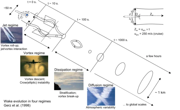
It is worth observing that these parameterizations are not meant to reproduce the actual evolution of exhaust plumes. In fact, the resolution used in large-scale models (a few hundred kilometers) does not allow to resolve the dynamical and physico-chemical processes occurring at the scales of the plume (which range from meters 10

to a few kilometers once trace gases get mixed with background). This is shown for example in Fig. 1 which sketches the dispersion of exhausts in aircraft plumes according to the representation proposed by Gerz et al. (1998). The process is initially driven by the dynamics of the wake vortices generated by the airplane (primary vortex pair). During the first few seconds after emission, the exhaust material is trapped 15

around the wake vortices (jet regime), which later start to sink by the mutually induced downward velocity (vortex regime). Part of the exhausts is detrained into a secondary vortex pair that forms due to the buoyancy force induced by atmospheric stratification while the majority of exhausts undergoes a complex instability process that leads to the vortex break-up, turbulence production and release of exhausts in the atmosphere 20

(dissipation regime). In the final diffusion regime the exhausts get diluted to background level via atmospheric processes (turbulence, radiation transport, etc.) usually within 2 to 12 h.

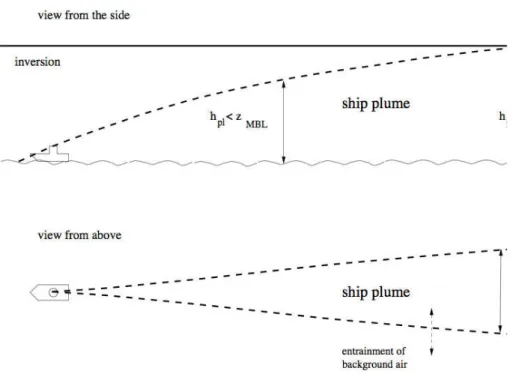
Ship plumes are another example of plumes from concentrated sources (see the sketch in Fig. 2). In this case the exhausts are released at the ship stack and initially 25

(8)

GMDD

4, 137–196, 2011

R. Paoli et al.

Title Page

Tables Figures

◭ ◮

Back Close

Full Screen / Esc

Discussion

P

a

per

|

Dis

cussion

P

a

per

|

Discussion

P

a

per

|

Discussio

n

P

a

per

|

disperse in the vertical direction before reaching the top of the marine boundary layer. Afterwards, the dispersion takes place mostly in the horizontal direction until complete dilution. This process can strongly depend on the background conditions and in particular on the typology of the boundary layer as well as the initial buoyancy flux at the stack of the ship (Chosson et al., 2008).

5

The most accurate way to model the evolution of reactive species in such complex scenarios is to rely on three-dimensional large-eddy simulations (LES) that cover the entire lifetime of the plume. However, although feasible, these simulations are still extremely demanding of computational resources – CPU power, memory and data storage – especially if several cases have to be run for a number of different conditions. 10

High-resolution LES of reactive wakes may require up to several million grid-points for tens of seconds to minutes plume age simulations (Lewellen and Lewellen, 2001a,b; Paoli et al., 2004; Chosson et al., 2008; Paugam et al., 2010). As detailed in the following sections, the alternative to such expensive three-dimensional simulations is

to rely on plume parameterizations that provide surrogates forEekff orK

e_ff

j . Then, data

15

from detailed LES or from experiments can be used to calibrate these parameters.

3 Representation of plume processes

This section examines the different models that have been developed in the literature to parameterize the processes occurring in plumes like those sketched in Figs. 1 and 2. The common feature of these models is that they use a finite (generally small) number 20

of parameters to represent the structure of the plume and the distribution of exhausts within it. These parameters evolve in time and obey ordinary differential equations (i.e., they do not explicitly depend on space), so in this sense all these models are zero-dimensional. Examples of key parameters are the mean concentration within the plume in Gaussian plume models, or the mean concentration within radial sectors of 25

the plume in Multilayered Plume models that will be described below. An important aspect that di_fferentiate these models is the way of representing the mixing in the

(9)

GMDD

4, 137–196, 2011

R. Paoli et al.

Title Page

Tables Figures

◭ ◮

Back Close

Full Screen / Esc

Discussion

P

a

per

|

Dis

cussion

P

a

per

|

Discussion

P

a

per

|

Discussio

n

P

a

per

|

interior of the plume and the entrainment of ambient air. To avoid confusion with the symbolsCk defined in Sect. 2 that pertain to large-scale Chemical Transport Models,

the concentrations obtained from small-scale plume models will be denoted by low-case symbolsc_k.

3.1 Instantaneous Dispersion (ID)

5

This simple parameterization represents the way emissions are usually handled in global models: the emissions are instantaneously diluted to the scales of a large control volume (e.g., the computational cell of a global model). Since this parameterization does not require any plume specification, only one set of ordinary di_fferential equations for the mean concentrationscID_k within the control volume is then sufficient to represent 10

the process:

d cID_k

d t =Ek,t0+ωk

cID₁ ,...,cID_N s

(13)

where the first term in the right-hand side means that emissions are non-zero only at timet=t0while the chemical sourcesωk obey the same law as in Eq. (2).

3.2 Single plumes

15

In the Single Gaussian Plume model, two sets of ordinary differential equations are solved: one for the mean concentration inside the plumecp_kand one for the background concentrationca_k:

d cp_k

d t =Ek,t0+ωk

cp₁,...,cp_N s

+cp_k−ca_k 1 Vp

d Vp

d t (14)

d ca_k

d t =ωk c

a 1,...,c

a

n

(15) 20

(10)

GMDD

4, 137–196, 2011

R. Paoli et al.

Title Page

Tables Figures

◭ ◮

Back Close

Full Screen / Esc

Discussion

P

a

per

|

Dis

cussion

P

a

per

|

Discussion

P

a

per

|

Discussio

n

P

a

per

|

whereVpdenotes the volume of the plume. In the case of aircraft emissions, plume is

asymmetric and anisotropic at cruise altitude because of atmospheric stratification and wind shear. A classical way of defining the dispersion of the plume is using a matrix of variances that follow a Gaussian distribution in the plane perpendicular to the flight path:σhandσvfor the horizontal and vertical variances, andσsthe diagonal term of the

5

matrix accounting for the deformation of the plume by vertical wind shear. Analytical solutions for these variances were obtained by Konopka (1995):

σ_h2=σ_h2_,₀+2sσ_s2_,₀+Dh

t+2sDs+s2+σv2,0

t2+2 3s

2_D

vt3 (16)

σv2=σ_v2_,₀+2Dvt (17)

σ_s2=σ_s2_,₀+sσ_v2_,₀+2Ds

t+sDvt2 (18)

10

whereD_v, D_h and D_s denote the vertical, horizontal, and shear diffusion coefficients, respectively, whiles denotes the wind shear. The subscript 0 in the above equations refer to a plume age t0 when the expansion of the plume can be approximated by

a pure diffusion process (typically the beginning of the diffusion regime as discussed in the previous section). The emissions in Eq. (14) should also be interpreted as already 15

diluted at the spatial scale of the plume corresponding tot0. Table 1 summarizes the

values of coefficients in Eqs. (16)–(18) obtained from in situ measurements (Schumann et al., 1995). The volume of the plume and the cross-sectional areaApcan be obtained

from Eqs. (16)–(17) as (Konopka, 1995):

Ap(t)=n2π

σ_h2σv2−σs4 1/2

(19) 20

Vp(t)=Ap(t)Lpath (20)

whereLpath denotes a reference length along flight direction, e.g., the distance flown

by the aircraft per second,Lpath=250 m at cruise speed (Kraabøl et al., 2000b), while

(11)

GMDD

4, 137–196, 2011

R. Paoli et al.

Title Page

Tables Figures

◭ ◮

Back Close

Full Screen / Esc

Discussion

P

a

per

|

Dis

cussion

P

a

per

|

Discussion

P

a

per

|

Discussio

n

P

a

per

|

the width of the plume. For example, choosingn=2 corresponds to incorporate 98% of exhaust (Petry et al., 1998).

In the case of ship emissions, the vertical and horizontal variances of the plume (with respect to the ship direction) can be derived by matching Gaussian solutions to empirical dispersion parameters (Seinfeld and Pandis, 2006). For example, Hanna 5

et al. (1985) and Song et al. (2003) determinedσh andσv by the standard deviations

of turbulent velocity fluctuations and the integral time scales of turbulence whereas von Glasow et al. (2003) proposed the simpler expressions

σh=σh,0 _t

t0 α

(21)

σv=σv,0 _t

t0 β

(22) 10

where subscript 0 identifies a reference time, for examplet0=1 s after emission, while

α and β are are the plume expansion rates that depend on the specific atmospheric conditions. von Glasow et al. (2003) also provided “best guest values” of 0.75 and 0.6 for α and β, respectively, based on the work by Durkee et al. (2000) (see also Table 2). Once the variances are specified, the ship plume area can be reconstructed 15

using Eq. (19) (with σs≡0), in particular taking n=1/ √

8, gives Ap=π/8σhσv which

corresponds to a semi-elliptical cross-section (von Glasow et al., 2003).

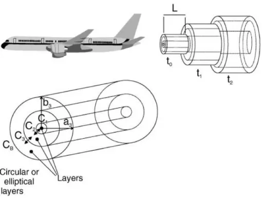
The Multilayered Plume model was first developed by Melo et al. (1978) and Vil `a-Guerau de Arellano et al. (1990) as a generalization of the single plume model for aircraft emissions. The plume is indeed divided into Nl concentric rings or layers

20

in order to represent the concentration distributions (see Fig. 3). A number of rings 4<N_l<16 has been typically used in the literature (Melo et al., 1978; Meijer, 2001; Kraabøl et al., 2000b; Vohralik et al., 2008). In this model, Eqs. (14)–(15) are replaced by the following set of equations for the mean concentrationcl_k inside each ringl of the

(12)

GMDD

4, 137–196, 2011

R. Paoli et al.

Title Page Abstract Introduction Conclusions References Tables Figures ◭ ◮ ◭ ◮ Back Close

Full Screen / Esc

Printer-friendly Version Interactive Discussion Discussion P a per | Dis cussion P a per | Discussion P a per | Discussio n P a per | plume:

d cl_k

d t =Ek,t0+ωk

cl₁,...,cl_N s

+fc1_k,...,cNl

k ;A1,...,ANl

1

Vp

d Vp

d t (23)

where A_l and V_l≡A_lLpath are, respectively, the area and the volume of the ring;

Vp= PNl

l=1Vl, while f is a function that parameterizes the mixing of species across

di_fferent layers of the plume (Meijer, 2001; Kraabøl et al., 2000b). The concentration 5

in the outermost layer corresponds to the ambient concentration, cNl

k ≡c

a

k, while the

overall mean concentration in the plume is given by

cp_k=

PNl

l=1c

l kVl

PNl

l=1Vl ≡

PNl

l=1c

l kVl

Vp

. (24)

It is interesting to rewrite the last term in the right-hand side of Eqs. (14) or (23) in terms of the entrainment rateωEor its inverse, the entrainment timeτE:

10

ωE≡

1 τE

= 1 Vp

d Vp

d t (25)

which represents the instantaneous expansion rate of the plume whose evolution can be computed analytically using Eqs. (16)–(20). The above equation suggests that in the limitτE→0, the plume concentration c

p

k relaxes instantaneously towards the ambient

concentrationca_k (see Eq. 15 or 23): in this case the single plume models degenerate 15

into the instantaneous dispersion model and Eq. (13) is recovered. It is worth remarking thatτE is a measure of the instantaneous dilution of the plume and, as such, it does

not provide any indication about thelifetime of the plume, which is a measure of the timescale over which exhausts can be considered diluted to background level. As discussed in the next section, this point is particularly relevant to the parameterization 20

of plume processes into global models whose spatial and temporal resolutions do not allow to reproduce the entire evolution of the plume.

(13)

GMDD

4, 137–196, 2011

R. Paoli et al.

Title Page

Tables Figures

◭ ◮

Back Close

Full Screen / Esc

Discussion

P

a

per

|

Dis

cussion

P

a

per

|

Discussion

P

a

per

|

Discussio

n

P

a

per

|

3.2.1 Choice of the plume lifetime

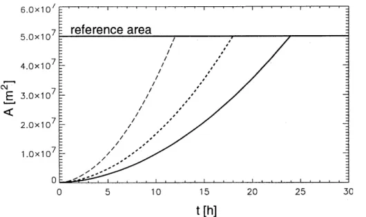
In the literature, various definitions have been proposed for the plume lifetimetp. Petry

et al. (1998) suggested to take

tp≡tref (26)

wheretrefis the “dispersion” time, i.e., the time when the plume reaches the dimensions

5

of a reference area Aref, for example the 2-D latitude-longitude grid box of a global

model (see Fig. 4). For typical grid resolutions employed in CTM,Aref≃5×10 7

m2 and tref≃18 h although this value strongly depends on the actual resolution of the global

model and on the dispersion parameters of the atmosphere. Meijer (2001), Karol et al. (2000) and Kraabøl et al. (2000b) defined the plume lifetime as

10

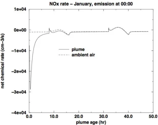
tp≡tmix (27)

where tmix represents the “mixing” time, i.e., the time when the NOx chemical

conversion rate in the plume and in the ambient air are sufficiently close (in practice, when the difference falls below a small threshold value, see Fig. 5). As shown by Karol et al. (2000), this time can vary significantly with the background conditions, the 15

characteristics of the atmospheric turbulence and the location of the plume, e.g., if it is inside or outside a flight corridor. Kraabøl et al. (2002) chose the life time as the minimum between the dispersion and the mixing times:

t_p_≡MIN(t_ref,t_mix). (28)

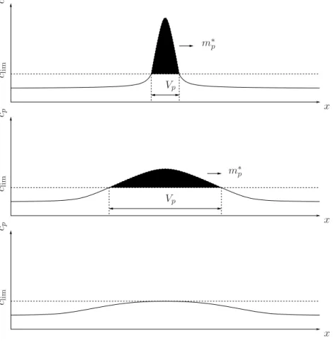
A rather di_fferent approach has been developed by Cariolle et al. (2009) to represent 20

plume dilution. This is based on the fact that the non-linear chemical processes within the plume are efficient up to a threshold value of exhaust concentrationclim. The plume

is then constituted by the air masses with concentration in excess with respect toclim:

Vp=V :c−clim>0, (29)

(14)

GMDD

4, 137–196, 2011

R. Paoli et al.

Title Page

Tables Figures

◭ ◮

Back Close

Full Screen / Esc

Discussion

P

a

per

|

Dis

cussion

P

a

per

|

Discussion

P

a

per

|

Discussio

n

P

a

per

|

m∗

p= Z

V_p

(c−clim)d Vp (30)

wherecindicates the concentration of a conserved species in the plume (e.g., NOx)

andV is a control volume. The excess of exhaust massm∗p decreases monotonically

in time until it gets to zero att=tlimas sketched in Fig. 6. This time is then taken as the

plume lifetime: 5

tp=tlim. (31)

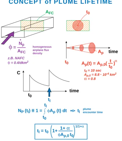
All the definitions of plume lifetime introduced above, Eqs. (26)–(31), implicitly assume that plumes do not overlap. However, in regions of dense traffic individual plumes can merge and the air masses with high exhaust concentration can have longer lifetime. Meilinger et al. (2005) determined the average plume encounter timetenchours for the

10

North Atlantic Flight Corridor (NAFC), which is an “objective” definition of plume lifetime in the sense that it does not depend on a specific plume or global model but only on the average aircraft flux density (see Fig. 7). The Single Plume or the Multilayered Plume models should be strictly valid only if the diffusion process is efficient enough fortrefortmixto be lower than the average plume encounter timetenc. This is generally

15

satisfied: for example, Petry et al. (1998) and Meijer (2001) found tref∼18 h and

tmix∼15 h, respectively, whereas tenc∼48 h (Meilinger et al., 2005). Similarly, in the

approach proposed by Cariolle et al. (2009), the plume size and lifetime depend on the mixing properties of the atmosphere and on the threshold valueclimchosen for exhaust

concentration. In the case of NOx, this threshold is clim∼1 ppb and the corresponding

20

tlim∼15 h, which, again, is much lower thantenc.

4 Parameterizations of emissions into global models

The plume models described above and 3-D large-eddy simulations can represent the evolution of the plume at the di_fferent levels of sophistication. However, because of the

(15)

GMDD

4, 137–196, 2011

R. Paoli et al.

Title Page

Tables Figures

◭ ◮

Back Close

Full Screen / Esc

Discussion

P

a

per

|

Dis

cussion

P

a

per

|

Discussion

P

a

per

|

Discussio

n

P

a

per

|

difference of scales and representation of physical processes, it would be unrealistic to integrate all the information carried by these small-scale models into large-scale CTM. For these reasons, a number of simpler parameterizations have been developed in the literature that attempt to reconstruct a limited number of parameters from small-scale models that can be e_fficiently used in CTM.

5

4.1 Effective Emission Indexes (EEI)

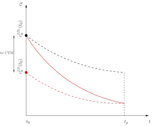
The concept of Effective Emission Indexes (EEI) was introduced by Petry et al. (1998) to provide corrections to instantaneous dispersion (ID) models where the emitted species are distributed instantaneously and homogeneously over the grid-box of large-scale models. Effective emissions are determined by varying the emissions obtained 10

with ID models and by comparing the corresponding results obtained with a Single Plume model (or Multilayered plume model) at the plume lifetimetp≡tref (see Eq. 26)

as sketched in Fig. (8). This procedure provides the variation∆c∗_k(t0) that has to be

added to the initial excess of concentration over background,

c∗ID

k (t0)≡c

p

k(t0)−ca_k, (32)

15

to retrieve the correct value at=tp. Once this variation is known, the initial excess of

concentrationc∗_kID(t0) is replaced by the corrected excessc

∗ID_corr

k (t0) defined as:

c∗IDcorr

k (t0)=c∗_kID(t0)+ ∆c∗_k(t0). (33)

To guarantee the conservation of the modified nitrogen mass of emitted species like NOx, an effective emission index of non-emitted or secondary species like ozone has

20

to be introduced. Then, to obtain maximum agreement with plume model results, a minimization procedure is applied to the root mean square deviationF:

F=

v u u u t

n

X

i=1 



c∗IDcorr

k (tp)−c∗_k(tp)

c∗_k(tp)



 2

. (34)

(16)

GMDD

4, 137–196, 2011

R. Paoli et al.

Title Page

Tables Figures

◭ ◮

Back Close

Full Screen / Esc

Discussion

P

a

per

|

Dis

cussion

P

a

per

|

Discussion

P

a

per

|

Discussio

n

P

a

per

|

For emitted species ke like NOx, the Effective Emission Index is obtained by simply

rescaling the standard Emission Index so as to take into account the correction in Eq. (33):

EEI_k_e(t0)=

1+δrel(ke)

EI_k_e (35)

where 5

δrel(ke)≡

∆c∗_k e(t0) c∗ID

k_e (t0)

(36)

is the relative correction of exhaust species concentrations. For secondary or non-emitted speciesknelike ozone, Effective Emission Indices are defined by rescaling the

NO_xEmission Index as

EEI_k

ne(t0)=δrel(kne)EINOx (37)

10

where

δrel(kne)=

W_k_ne WNO_x

∆c∗_k ne(t0) c∗ID

NO_x(t0)

(38)

is the relative correction of secondary species concentrations with respect to NO_x, while Wk denotes the molecular weight of species k. Petry et al. (1998) computed

the EEI by means of their Single Plume model that employs the Chemistry Module for 15

the Lower Stratosphere and the Troposphere (CHEST). This chemical mechanism is based on the EURAD model system (Hass, 1991) and considers the transformations of 160 species by 160 homogeneous gas phase collision reactions and 26 photolysis reactions (Stockwell, 1986; Stockwell et al., 1990). Figure 9 shows a good agreement between the c∗IDcorr

k (tp) and c∗k(tp) for the absolute changes of some key species,

20

meaning that that Eq. (33) allows the concentrations of the instantaneous dispersion model to recover the correct plume model concentrations at the end of the plume

(17)

GMDD

4, 137–196, 2011

R. Paoli et al.

Title Page

Tables Figures

◭ ◮

Back Close

Full Screen / Esc

Discussion

P

a

per

|

Dis

cussion

P

a

per

|

Discussion

P

a

per

|

Discussio

n

P

a

per

|

lifetime. Figure 10 reports the time evolution of∆c∗_kfor different background conditions. As a general remark, Petry et al. (1998) found that the corrections to the concentration obtained with the standard ID method can vary significantly, depending on release time and the degree pollution of the background environment. In particular, negative NOy

and ozone effective emission indexes were obtained for some specific release times. 5

Franke et al. (2008) recently applied the EEI method to ship emissions using the plume dispersion formulation by Song et al. (2003) and the photochemical box model MECCA (Sander et al., 2005), which includes 160 gas-phase reactions in addition to 116 aqueous, 61 heterogeneous and 42 equilibrium reactions for sulfur and sea-salt aerosols. Both primary emissions and secondary emissions for ozone and H₂O₂ and 10

the corrections of NOx were balanced by effective emissions of HNO3, PAN and

sea-salt aerosol nitrate. They observed that the original NOx emissions were reduced by

about 3%, while ozone and H₂O₂were, respectively, reduced by 700% and increased by 5% the amount of emitted NOx (see Fig. 11). As expected, the relative emission

indexes are always negative due to the fact that they correct the ozone overestimation 15

of the ID model box. The e_ffective emissions of O₃are largest for release times during day and smallest during night.

Once the EEI are computed, the “effective” emissions in the CTM mass balance equations are reconstructed as

Ee_kff=EEI_k(t₀)S_f (39)

20

which formally replaces Eq. (8).

4.2 Emission Conversion Factors (ECF)

The method of Emission Conversion Factor (ECF) proposed by Meijer et al. (1997), Meijer (2001) attempts to determine the local conversions of the emitted species on the same plume, rather than forcing emissions from ID model to follow those of SP 25

models, as sketched in Fig. 12. For emitted species, Meijer (2001) introduced the

(18)

GMDD

4, 137–196, 2011

R. Paoli et al.

Title Page

Tables Figures

◭ ◮

Back Close

Full Screen / Esc

Discussion

P

a

per

|

Dis

cussion

P

a

per

|

Discussion

P

a

per

|

Discussio

n

P

a

per

|

excess of mass over background as the difference between the number of molecules in the control volume with and without the aircraft plume:

m∗_k

e(t)=Vp(t)

cp_k e(t)−c

a

ke(t)

(40)

while, for non-emitted species the excess of mass is given by

m∗

k_ne(t)=Vp(t)c p

k_ne(t). (41)

5

The ECF is then defined as the ratio between the emissions of specieskand that of all nitrogen oxides NO_y(which is constant in time since NO_yare chemically conserved):

ECF_k(t)= m

∗ k(t)

m∗_NO y(t)

= c

p

k(t)−c

a

k(t)

cp_NO y(t)−c

a NO_y(t)

. (42)

The Multilayered Plume model used to compute the ECF is described in detail in Meijer (2001). The photochemical mechanism for the troposphere contains 44 species and 10

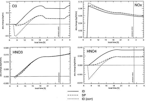
103 reactions, and is adapted from Strand and Hov (1994), with gas-phase reaction rates taken from De More et al. (1997) and microphysics from K ¨archer (1997). The background conditions correspond to typical values encountered along the NAFC at an altitude of about 10.5 km (250 hPa), at different times (respectively 8 a.m. and 12 a.m.) and different seasons (January and July). The ECF are reported in Fig. 13: 15

as expected, ECFNO_x decreases while ECFO₃ increases as NOx is converted in the

plume. For all cases, the net chemical rates of NO_x and O₃ in the plume shows large destruction rate during the first hours, whereafter the net rate slowly converges to the net rate in the ambient air (around 10 h). A value oftp≡tmix=15 h (see Eq. 27) was then

suggested as a conservative choice for the plume lifetime. 20

A similar approach was used by Kraabøl et al. (2000b) and Kraabøl and Stordal (2000). One difference is that their chemistry scheme, taken from Kraaøbl et al. (1999), contains 66 species and 170 reactions, providing a complete description of the free-atmosphere. In addition, their analysis showed that the NO_x conversion rates

(19)

GMDD

4, 137–196, 2011

R. Paoli et al.

Title Page

Tables Figures

◭ ◮

Back Close

Full Screen / Esc

Discussion

P

a

per

|

Dis

cussion

P

a

per

|

Discussion

P

a

per

|

Discussio

n

P

a

per

|

were most sensitive to the diurnal, seasonal and latitudinal variations of background conditions (see e.g., Fig. 14), and then suggested that such variations should be taken into account for the integration in global models. Vohralik et al. (2008) recently tested the ECF technique and confirmed the strong dependence of NOxconversion into NOy

on altitude, latitude and seasonal variations (see Fig. 15). 5

The “effective” emissionsEekffin the CTM mass balance equations are reconstructed

by rescaling the emissions by the ECF evaluated at the plume lifetimetp:

Ee_kff=ECF_k(tp)Ek. (43)

4.3 Plume Transformation Indices (PTI) and Effective Perturbation Indices (EPI)

In the methodology proposed by Karol et al. (2000) the effective emission index is 10

decomposed in two factors: the usual emission index that quantifies the in-engine processes (EI) and the dimensionless Plume Transformation Index (PTI):

EEIk=EIk×PTIk (44)

This method follows the idea of Petry et al. (1998) of modifying the emission indices but it represents the variation of the total mass (or the number of molecules) of species 15

by an integration over the entire plume lifetime rather than an evaluation attpas in the

ECF method by Meijer (2001). Subtracting Eq. (15) from Eq. (14) and integrating over t_pyields after some algebra to:

∆m∗ k(tp)=

tp Z

t₀

Vp(t) h

ωp_k(t)₋ωa_k(t)id t=m∗

k(tp)−m∗_k(t0) (45)

where Eq. (40) has been used. For emitted specieskethe PTI is defined as

20

PTI_k

e(t0,tp)=

Vp(t0)c p

k_e(t0)+ ∆m∗k_e(tp)

V_p(t₀)cp_k e(t0)

(46)

(20)

GMDD

4, 137–196, 2011

R. Paoli et al.

Title Page

Tables Figures

◭ ◮

Back Close

Full Screen / Esc

Discussion

P

a

per

|

Dis

cussion

P

a

per

|

Discussion

P

a

per

|

Discussio

n

P

a

per

|

while for speciesknenot emitted by the aircraft and originating in plume from interaction

with the emitted specieske, the PTI is given by

PTI_k

ne(t0,tp)= m∗_k

ne(tp) Vp(t0)c

p

k_ne(t0)

. (47)

The plume model developed by Karol et al. (1997) was used to get the PTIk. The

chemistry scheme included 85 gas phase reactions and 33 compounds without 5

heterogeneous chemistry. The plume simulations took place in the 9–12-km layer at 50◦and 30◦N in the upper troposphere and lower stratosphere inside and outside the NAFC, in January and July. The calculations of PTI confirmed the conclusions given by Meijer et al. (1997) and Petry et al. (1998) that a significant part of NO_xcomponents emitted by subsonic aircraft may be transformed into the NOycomponents in the plume

10

stage, and that these transformations are mostly sensitive to ambient air composition (see for example Fig. 16). In particular, Karol et al. (2000) observed that flying in the warm stratosphere and out of flight corridor should reduce the released NOx entering

into large-scale and the global reservoir of the aircraft NOy.

Meilinger et al. (2005) developed a detailed plume model to analyze the 15

microphysical processes and heterogeneous chemistry in aircraft plumes, including the formation of persitent contrails. For emitted species, they used the definition of PTI in Eq. (46) while for non emitted species, they introduced a slightly different definition, named E_ffective Perturbation Index:

EPI_k ne=

cp_k

ne(tenc)−c

a

k_ne(tenc)

ca_k ne(tenc)

(48) 20

where tenc is the average plume encounter time in the NAFC (see Sect. 3.2.1).

The simulations confirmed the high sensitivity of NO_x conversion and ozone formation/depletion on meteorological conditions, including relative humidity which affects the persistence of contrails (see Fig. 17).

(21)

GMDD

4, 137–196, 2011

R. Paoli et al.

Title Page

Tables Figures

◭ ◮

Back Close

Full Screen / Esc

Discussion

P

a

per

|

Dis

cussion

P

a

per

|

Discussion

P

a

per

|

Discussio

n

P

a

per

|

The “effective” emissionsEe_kffin the CTM mass balance equations are reconstructed using Eqs. (8), (44) and (46)–(47)

Ee_kff=EI_kPTI_k t0,tp

Sf. (49)

4.4 Effective Reaction Rates (ERR)

The method of effective reaction rates (ERR) was introduced by Cariolle et al. (2009) 5

to study the impact of NOxemissions on the atmospheric ozone. The basic idea of the

method is that the chemical transformations in the plume proceed with different rates than in the background atmosphere because of the high concentrations of exhausts within the plume. It is then possible to define “effective” reaction rate constants working on the fraction of the emissions within the plume (undiluted fraction). To discriminate 10

between diluted and undiluted fractions of emissions, an additional transport equation for a fuel tracer is solved by the CTM:

DCf

Dt =Sf− Cf

τ (50)

where the last term in the right-hand side is a model for the (large-scale) fuel dilution. The decay timeτis obtained by approximating the evolution of excess of exhaust mass 15

m∗pin Eq. (30) by an exponential fit: m∗p(t)=m∗p(t0)exp(−(t−t0)/τ) so that

τ≡

+∞

Z

t₀

e−(t−t0)/τ_{d t}₌ 1 m∗p(t0)

tp Z

t₀

m∗p(t)d t (51)

where tp=tlim is defined according to the threshold value clim as explained in

Sect. 3.2.1. The (grid-averaged) undiluted fraction of NO_x (exhaust NO_x) is reconstructed usingCfas

20

CpNO_x=αNO_xEINO_xCf (52)

(22)

GMDD

4, 137–196, 2011

R. Paoli et al.

Title Page

Tables Figures

◭ ◮

Back Close

Full Screen / Esc

Discussion

P

a

per

|

Dis

cussion

P

a

per

|

Discussion

P

a

per

|

Discussio

n

P

a

per

|

where αNO_x=10− 3

Wair/WNO_x is a scaling factor with Wair and WNO_x the molecular

weights of air and NOx, respectively.

To account for the e_ffects of highly concentrated exhaust NO_x on ozone concentration, an “effective” reaction rate is introduced as:

KeNOff _xO₃=

t_p

R

t₀

R

Vp

KNO_xO₃cNO_xcO₃d Vp !

d t

ca_O 3

t_p

R

t0 R

V_p

cNO_xd Vp !

d t

(53) 5

where the plume concentrations can be obtained using any of the plume models introduced in Sect. 3 or explicit three-dimensional LES. The ozone balance equation in the CTM is modified by adding a term which represents the destruction of ozone by

NOxat the scale of the grid-box and proceeds at the rateK eff

NO_xO₃:

DCO₃

Dt =ωO3(C1,...,CNs)−K

eff

NO_xO₃C p

NO_xCO₃. (54)

10

This approach is slightly different from the general formulation of effective reactions

introduced in Eq. (12) in the sense thatKeNOff_xO₃ is constructed in such a way that the

grid-averaged undiluted fractionCpNO_x rather than the total grid-averaged concentration

CNO_x appear explicitly in the ozone balance equation. The EER method gives

a framework that is fully conservative for the injected species, and that relaxes to 15

ID model when τ→0. It was found that the NOx-ozone chemistry inside the plume

is characterized by a first regime during which NO and NO₂ get to equilibrium while ozone decreases by titration of NO2, and by a following slower decrease of odd oxygen

NO2+O3species (see Fig. 18). Cariolle et al. (2009) further discuss the determination

(23)

GMDD

4, 137–196, 2011

R. Paoli et al.

Title Page

Tables Figures

◭ ◮

Back Close

Full Screen / Esc

Discussion

P

a

per

|

Dis

cussion

P

a

per

|

Discussion

P

a

per

|

Discussio

n

P

a

per

|

of KeNOff _xO₃ for ozone and the values of tp and τ, and introduce additional terms to

account for O₃titration and the formation of nitric acid during the plume dilution.

5 Integration of emission parameterizations into global models

This section describes the results of the implementation of the different parameteriza-tions presented in Sect. 4 into global and regional models. In order to evaluate the 5

effects of plume processes, three baseline computations can be designed:

– run A: with the unmodified emission inventories for NO_x and other exhaust species

– runB: with the modified emissionsEekffor reaction ratesK

eff

j

– runC: without emissions 10

The perturbations due to the chemical conversions are then quantified in absolute numbers:

εk=Ck(runA)−Ck(runB) (55)

and relative numbers:

ε_k_%=Ck(runA)−Ck(runB) C_k(runB)−C_k(runC)×

100. (56)

15

5.1 Application of ECF and EEI

The ECF were first implemented by Meijer et al. (1997) in the Chemistry Transport Model CTMK (Velders et al., 1994; Wauben et al., 1997) and successively by Meijer (2001) in the TM3 model (Meijer et al., 2000). The original engine exit emissions from

(24)

GMDD

4, 137–196, 2011

R. Paoli et al.

Title Page

Tables Figures

◭ ◮

Back Close

Full Screen / Esc

Discussion

P

a

per

|

Dis

cussion

P

a

per

|

Discussion

P

a

per

|

Discussio

n

P

a

per

|

the DLR/ANCAT 2 NO_xemissions (Gardner et al., 1997) were transformed into aircraft plume emissions using the ECF in Eq. (43) at each computational cell. The plume lifetime was takentp=15 h (Meijer, 2001).

Figure 19 shows the monthly mean of absolute and relative NO_x and O₃ perturbations. As expected, the main NOx perturbations were along the main aircraft

5

routes, with mean values of 50–100 pptv in January, and 50–110 pptv in July in the case of unmodified ANCAT emissions. The O₃ perturbations around and in the main flight corridors were in the range of 1.8–2.1 ppbv for January and 2–3.8 ppbv for July. When the ECF parameterization was included NOxperturbations were reduced by 15–30 pptv

in January, and by 10–35 pptv in July (in relative numbers, these reductions amount to 10

20–30% and 20–40%, respectively). Generally, the ozone perturbation is reduced due to the efficient conversion of NOx in the aircraft plumes, leading to a diminished O3

production on the global scale. On the other hand, the photochemistry in the aircraft exhaust plumes generally produces additional ozone emissions. If photochemical activity is sufficiently high, net ozone production in the aircraft plumes can be large 15

enough to enhance the aircraft-induced ozone perturbation. This explains the increase (negative reduction) of the local perturbation of ozone in the NAFC for July. The maximal enhancement was 8% (note that the results presented by Meijer (2001) are slightly different from those of Meijer et al. (1997) because the net ozone production and the time of emission had not been taken into account).

20

Kraabøl et al. (2000a) implemented the ECF methodology into NILU-CTM, a three-dimensional chemistry transport meso-scale model covering Europe, North America, and the North Atlantic (Flatøy et al., 1995; Simpson, 1992; Strand and Hov, 1994). The spatial distribution of aircraft NOx emissions were taken from the DLR/ANCAT 2

(Gardner et al., 1997). The plume lifetime for the implementation of ECF was taken 25

tp=15 h, which, in this case, also corresponds to a plume width of approximately the

size of the computational cell. Without plume modifications, the monthly averaged increases for July for NOx and ozone were up to 70 ppt and 2.7 ppb, respectively. On

the other hand, with plume modifications, the corresponding NO_xand ozone increases

(25)

GMDD

4, 137–196, 2011

R. Paoli et al.

Title Page

Tables Figures

◭ ◮

Back Close

Full Screen / Esc

Discussion

P

a

per

|

Dis

cussion

P

a

per

|

Discussion

P

a

per

|

Discussio

n

P

a

per

|

were reduced by 30 ppt (_∼40%) and 0.5 ppb (_∼20%), respectively (see Fig. 20). The ozone increase within the North Atlantic Flight Corridor (NAFC) was also reduced by up to 0.5 ppb (∼30%).

Kraabøl et al. (2002) implemented the plume model into the OSLO-CTM2 (Sundet, 1997), which is based on the chemical scheme described by Hesstvedt et al. (1978) 5

and Berntsen and Isaksen (1999). The implementation of ECF is very similar to that used by Kraabøl et al. (2000a), expect that the variations in the turbulent conditions of the atmosphere were taken into account: following D ürbeck and Gerz (1996), the diffusivities needed by the plume model, Eqs. (16)–(18), where reconstructed in each computational cell using the probability density function of Brunt-V äis äl ä frequencyN 10

and vertical wind shearsfrom the ECMWF forecast data in the Northern Hemisphere between 8 and 12 km. Furthermore, the plume was followed until either the size was considered large enough to be representative for the grid resolution of OSLO-CTM2 or the NO_xemissions were homogeneously mixed with the surrounding air, i.e. tp=MIN(tref,tmix), see Eq. (28) (a value of 48 h was taken as an upper limit).

15

When plume modifications with variable turbulence are included in the global model, the aircraft-induced NO_x and ozone increases in the NAFC and over Europe were reduced (see Fig. 21). The absolute (relative) reductions were strongest in April/May, where NOx and ozone decreased by 15 to 25 pptv (25–35%) and 0.8 to 1 ppbv

(15–18%) at northern midlatitudes, respectively. The corresponding numbers were 20

estimated to 8 to 22 ppt (20%) for NOx and 0.4 to 0.6 ppb (15–20%) for ozone in

January. Kraabøl et al. (2002) finally pointed out a few issues on the modeling of ECF of NO_x that deserve further investigation. The first issue concerns the assumption of stationary turbulence during the plume lifetime: for certain (weak) values ofN and s from ECMWF data, this may overestimate the dispersion time of the plume to reach the 25

resolved scale of the global model. In real atmosphere, the plume is likely to encounter conditions that favor much higher dispersion over that period. In this case the ozone production efficiency will be higher than that predicted by the simulations. The second issue is that the emissions were represented as a single plume, whereas in reality, the

(26)

GMDD

4, 137–196, 2011

R. Paoli et al.

Title Page

Tables Figures

◭ ◮

Back Close

Full Screen / Esc

Discussion

P

a

per

|

Dis

cussion

P

a

per

|

Discussion

P

a

per

|

Discussio

n

P

a

per

|

emissions within a computational cell of a CTM consist of multiple plumes. Mixing of multiple plumes causes a lower fraction of the emitted NOxto be converted into NOyin

the plume (Kraabøl et al., 2002). Thus, more NOxwill remain as NOxwhen the plume

reaches the resolved scale of the CTM. This will lead to a higher ozone production efficiency of emissions.

5

The EEI and ECF techniques were recently tested by Vohralik et al. (2008) using the same plume model and the CSIRO two-dimensional chemical transport model (Randeniya et al., 2002). The comparison between the two techniques showed significant differences in the predicted NOx increase although the aircraft-induced

ozone perturbations were found relatively small. In general, the predicted effects 10

on the global impact of ozone were comparable in magnitude to those found by Meijer (2001) but considerably smaller than those obtained by Kraabøl et al. (2002).

5.2 Application of ERR

The ERR method (Cariolle et al., 2009) has been implemented in the 3-D model LMDz-INCA (Hauglustaine et al., 2004; Folberth et al., 2006) coupled to the AERO2K 15

emission database (Eyers et al., 2004). Figure 22 shows that the large-scale NO_x content decreases significantly over the main flight corridors due to their storage in high-concentration plume form and to the conversion of a fraction of the NOx into

HNO₃. This large scale NO_x decrease reduces the background O₃ production that adds to the direct local O3destruction found within the plume air masses. The result is

20

a reduction of the global aircraft induced O3production by about 15% in the Northern

Hemisphere when the plume e_ffects are taken into account. This result is consistent with the evaluations made using the EEI and ECF methods.

The ERR method has been recently adapted by Huszar et al. (2010) to treat the case of NO_x emissions by ships within the near Atlantic European Corridor. The 25

simulations were carried out using the CAMX, an Eulerian photochemical dispersion model developed by ENVIRON Int. Corp. (http://www.camx.com) coupled to the