Implicit particle filtering for models with partial noise, and an application to geomagnetic data assimilation

www.nonlin-processes-geophys.net/19/365/2012/ doi:10.5194/npg-19-365-2012

© Author(s) 2012. CC Attribution 3.0 License.

Nonlinear Processes

in Geophysics

Implicit particle filtering for models with partial noise, and an

application to geomagnetic data assimilation

M. Morzfeld1and A. J. Chorin1,2

1_{Lawrence Berkeley National Laboratory, Berkeley, CA, USA}

2_{Department of Mathematics, University of California, Berkeley, CA, USA}

Correspondence to:M. Morzfeld (mmo@math.lbl.gov)

Received: 27 September 2011 – Revised: 22 May 2012 – Accepted: 22 May 2012 – Published: 19 June 2012

Abstract. Implicit particle filtering is a sequential Monte Carlo method for data assimilation, designed to keep the number of particles manageable by focussing attention on regions of large probability. These regions are found by min-imizing, for each particle, a scalar functionF of the state variables. Some previous implementations of the implicit fil-ter rely on finding the Hessians of these functions. The cal-culation of the Hessians can be cumbersome if the state di-mension is large or if the underlying physics are such that derivatives ofF are difficult to calculate, as happens in many geophysical applications, in particular in models with partial noise, i.e. with a singular state covariance matrix. Examples of models with partial noise include models where uncertain dynamic equations are supplemented by conservation laws with zero uncertainty, or with higher order (in time) stochas-tic partial differential equations (PDE) or with PDEs driven by spatially smooth noise processes. We make the implicit particle filter applicable to such situations by combining gra-dient descent minimization with random maps and show that the filter is efficient, accurate and reliable because it operates in a subspace of the state space. As an example, we consider a system of nonlinear stochastic PDEs that is of importance in geomagnetic data assimilation.

1 Introduction

The task in data assimilation is to use available data to update the forecast of a numerical model. The numerical model is typically given by a discretization of a stochastic differential equation (SDE)

xn+1=R(xn, tn)₊G(xn, tn)1Wn+1, (1) where x is an m-dimensional vector, called the state, tn, n₌0,1,2, . . ., is a sequence of times,Ris anm-dimensional vector function, Gis an m_×m matrix and1W is an m-dimensional vector, whose elements are independent stan-dard normal variates. The random vectorsG(xn, tn)1Wn+1

represent the uncertainty in the system, however even for G₌0 the state xn may be random for any n because the initial statex0can be random. The data

zl=h(xq(l), tq(l))₊Q(xq(l), tq(l))Vl (2) are collected at times tq(l),l₌1,2, . . .; for simplicity, we assume that the data are collected at a subset of the model steps, i.e.q(l)₌rl, withr_≥1 being a constant. In the above equation, z is a k-dimensional vector (k≤m), h is a k-dimensional vector function, V is a k-dimensional vector whose components are independent standard normal vari-ates, andQis ak_×kmatrix. Throughout this paper, we will writex0:n_{for the sequence of vectorsx}0_{, . . . ,x}n_.

Data assimilation is necessary in many areas of science and engineering and is essential in geophysics, for exam-ple in oceanography, meteorology, geomagnetism or atmo-spheric chemistry (see e.g. the reviews Miller et al., 1994; Ide et al., 1997; Miller et al., 1999; van Leeuwen, 2009; Bocquet et al., 2010; Fournier et al., 2010). The assimilation of data in geophysics is often difficult because of the complicated un-derlying dynamics, which lead to a large state dimensionm and a nonlinear functionRin Eq. (1).

and can be characterized in full by its mean and covariance. The Kalman filter (KF) sequentially computes the mean of the model (1), conditioned on the observations and, thus, pro-vides the best linear unbiased estimate of the state (Kalman, 1960; Kalman and Bucy, 1961; Gelb, 1974; Stengel, 1994). The ensemble Kalman filter (EnKF) is a Monte Carlo ap-proximation of the Kalman filter, and can be obtained by replacing the state covariance matrix by the sample covari-ance matrix in the Kalman formalism (see Evensen, 2007). The state covariance is the covariance matrix of the pdf of the current state conditioned on the previous state which we calculate from the model (1) to be

p(xn+1|xn)_∼N(R(xn, tn),G(xn, tn)G(xn, tn)T), (3) whereN(µ, 6)denotes a Gaussian with meanµand covari-ance matrix6. To streamline the notation we write for the state covariance:

6_xn₌G(xn, tn)G(xn, tn)T, (4) whereT denotes a transpose. In the EnKF, the sample covari-ance matrix is computed from an “ensemble”, by running the model (1) for different realizations of the noise process1W. The Monte Carlo approach avoids the computationally ex-pensive step of updating the state covariance in the Kalman formalism. Both KF and EnKF have extensions to nonlin-ear, non-Gaussian models, however they rely on linearity and Gaussianity approximations (Julier and Uhlmann, 1997).

Variational methods (Zupanski, 1997; Tremolet, 2006; Ta-lagrand, 1997; Courtier, 1997; Courtier et al., 1994; Bennet et al., 1993; Talagrand and Courtier, 1987) aim at assimilat-ing the observations within a given time window by comput-ing the state trajectory of maximum probability. This state trajectory is computed by minimizing a suitable cost func-tion. In particular, 3-D-Var methods assimilate one obser-vation at a time (Talagrand, 1997). Strong constraint 4-D-Var determines the most likely initial statex0given the data

z1,z2, . . . ,zl, a “perfect” model, i.e.G=0, and a Gaussian initial uncertainty, i.e. x0_∼N(µ0, 60) (Talagrand, 1997; Courtier, 1997; Courtier et al., 1994; Talagrand and Courtier, 1987). Uncertain models with G₆₌0 are tackled with a weak constraint 4-D-Var approach (Zupanski, 1997; Tremo-let, 2006; Bennet et al., 1993). Many variational methods use an adjoint minimization method and are very efficient. To further speed up the computations, many practical implemen-tations of variational methods, e.g. incremental 4-D-Var, use linearizations and Gaussian approximations.

For the remainder of this paper, we focus on sequential Monte Carlo (SMC) methods for data assimilation, called particle filters (Doucet et al., 2001; Weare, 2009; Moral, 1998; van Leeuwen, 2010; Moral, 2004; Arulampalam et al., 2002; Doucet et al., 2000; Chorin and Tu, 2009; Chorin et al., 2010; Gordon et al., 1993; Morzfeld et al., 2012). Particle filters do not rely upon linearity or Gaussianity assumptions and approximate the pdf of the state given the observations,

p(x0:q(l)_|z1:l), by SMC. The state estimate is a statistic (e.g. the mean, median, mode etc.) of this pdf. Most particle filters rely on the recursive relation

p(x0:q(l+1)|z1:l+1)_∝p(x0:q(l)|z1:l)

×p(zl+1_|xq(l+1))p(xq(l)+1:q(l+1)_|xq(l)). (5) In the above equationp(x0:q(l+1)_|z1:l+1)is the pdf of the state trajectory up to timetq(l+1), given all available obser-vations up to time tq(l+1) and is called the target density; p(zl+1|xq(l+1))is the probability density of the current ob-servation given the current state and can be obtained from Eq. (2)

p(zl+1|xq(l+1))_∼N(h(xq(l), tq(l)), 6_zn), (6) with

6_zn₌Q(xn, tn)Q(xn, tn)T. (7) The pdfp(xq(l)+1:q(l+1)|xq(l))is the density of the state trajectory from the previous assimilation step to the current observation, conditioned on the state at the previous assimi-lation step, and is determined by the model (1).

A standard version of the sequential importance sampling with resampling (SIR) particle filter (also called bootstrap filter, see e.g. Doucet et al., 2001) generates, at each step, samples fromp(xq(l)+1:q(l+1)_|xq(l)_{)(the prior density) by} running the model. These samples (particles) are weighted by the observations with weights w_∝p(zl+1_|xq(l+1)_{), to} yield a posterior density that approximates the target den-sityp(x0:q(l+1)_|z1:l+1). One then removes particles with a small weight by “resampling” (see e.g. Arulampalam et al., 2002 for resampling algorithms) and repeats the procedure when the next observation becomes available. This SIR fil-ter is straightforward to implement, however the catch is that many particles have small weights because the particles are generated without using information from the data. If many particles have a small weight, the approximation of the tar-get density is poor and the number of particles required for a good approximation of the target density can grow catas-trophically with the dimension of the state (Snyder et al., 2008; Bickel et al., 2008). Various methods, e.g. different prior densities and weighting schemes (see e.g. Doucet et al., 2001; van Leeuwen, 2010, 2009; Weare, 2009), have been in-vented to ameliorate this problem, but a rigorous analysis of how the number of particles scales with the dimension of the state space has not been reported for any of these methods.

the regions of high probability through a particle-by-particle minimization and then setting up an underdetermined alge-braic equation that depends on the model (1) as well as on the data (2), and whose solution generates a high probability sample of the target density. We review the implicit filter in the next section, and it will become evident that the construc-tion assumes that the state covariance6_xnin Eq. (4) is non-singular. This condition is often not satisfied. If, for example, one wants to assimilate data into a stochastic partial differen-tial equation (SPDE) driven by spadifferen-tially smooth noise, then the continuous-time noise process can be represented by a series with rapidly decaying coefficients, leading to a sin-gular or ill-conditioned state covariance6n_x in discrete time and space (see Sects. 3.1 and 4, as well as Lord and Rouge-mont, 2004; Chueshov, 2000; Jentzen and Kloeden, 2009). A second important class of models with partial noise are uncertain dynamic equations supplemented by conservation laws (e.g. conservation of mass) with zero uncertainty. Such models often appear in data assimilation for fluid dynamics problems (Kurapov et al., 2007). A similar situation occurs when second-order (in time) equations are formulated as sys-tems of first-order equations, e.g. in robotics.

The purpose of the present paper is two-fold. First, in Sect. 2, we present a new implementation of the implicit par-ticle filter. Most previous implementations of the implicit fil-ter (Chorin et al., 2010; Morzfeld et al., 2012) rely in one way or another on finding the Hessians of scalar functions of the state variables. For systems with very large state vectors and considerable gaps between observations, memory constraints may forbid a computation of these Hessians. Our new imple-mentation combines gradient descent minimization with ran-dom maps (Morzfeld et al., 2012) to avoid the calculation of Hessians, and thus reduces the memory requirements.

The second objective is to consider models with a singular or ill-conditioned state covariance6n_xwhere previous imple-mentations of the implicit filter, as described in Chorin and Tu (2009); Chorin et al. (2010); Morzfeld et al. (2012), are not applicable. In Sect. 3, we make the implicit filter applica-ble to models with partial noise and show that our approach is then particularly efficient, because the filter operates in a space whose dimension is determined by the rank of6n_x, rather than by the model dimension. We compare the new implicit filter to SIR, EnKF and variational methods.

In Sect. 4, we illustrate the theory with an application in geomagnetic data assimilation and consider two coupled nonlinear SPDEs with partial noise. We observe that the im-plicit filter gives good results with very few (4–10) particles, while EnKF and SIR require hundreds to thousands of parti-cles for similar accuracy.

2 Implicit sampling with random maps

We first follow Morzfeld et al. (2012) closely to review im-plicit sampling with random maps. Suppose we are given a

collection ofMparticlesXq(l)_j ,j ₌1,2, . . . , M, whose em-pirical distribution approximates the target density at time tq(l), whereq(l)₌rl, and suppose that an observationzl+1is available afterrsteps at timetq(l+1)₌tr(l+1). From Eq. (5) we find, by repeatedly using Bayes’ theorem, that, for each particle,

p(X_j0:q(l+1)_|z1:l+1)_∝p(X_j0:q(l)_|z1:l)p(zl+1_|Xq(l_j +1))

×p(Xq(l_j +1)|X_jq(l+1)−1)p(X_jq(l+1)−1|X_jq(l+1)−2) ..

.

×p(Xq(l)_j +1|Xq(l)_j ). (8) Implicit sampling is a recipe for computing high-probability samples from the above pdf. To draw a sample we define, for each particle, a functionFj by

exp(₋F (Xj))=p(Xq(lj +1)|X q(l+1)−1

j )···p(X

q(l)+1

j |X

q(l)

j )

×p(zl+1_|Xq(l_j +1)) (9)

whereXjis shorthand for the state trajectoryXq(l)_j +1:q(l+1). Specifically, we have

Fj(Xj)=1 2

Xq(l)_j +1₋Rq(l)_j T6q(l)_x,j

−1

Xq(l)_j +1₋Rq(l)_j

+₂1Xq(l)_j +2₋R_jq(l)+1T6_x,jq(l)+1

−1

Xq(l)_j +2₋Rq(l)_j +1

.. .

+1₂

X_jq(l+1)−R_jq(l+1)−1T6_x,jq(l+1)−1−1X_jq(l+1)−Rq(l+_j 1)−1

+1₂hX_jq(l+1)₋zl+1T6_z,jl+1−1hX_jq(l+1)₋zl+1

+Zj, (10)

whereRn_j is shorthand notation forR(Xn_j, tn)and whereZj is a positive number that can be computed from the normal-ization constants of the various pdfs in the definition ofFj in Eq. (9). Note that the variables of the functions Fj are Xj=Xq(l)_j +1:q(l+1), i.e. the state trajectory of thej-th parti-cle from timetq(l)+1totq(l+1). The previous position of the j-th particle at timetq(l),Xq(l)_j , is merely a parameter (which varies form particle to particle). The observationzl+1_{is the}

same for all particles. The functionsFj are thus similar to one another. Moreover, eachFj is similar to the cost func-tion of weak constraint 4-D-Var, however, the state at time tq(l)is “fixed” for eachFj, while it is a variable of the weak constraint 4-D-Var cost function.

reference variableξ_∼N_{(0,I), this can be done by solving}

the algebraic equation Fj(Xj)−φj=

1 2ξ

T

jξj, (11)

whereξjis a realization of the reference variable and where

φj =minFj. (12)

Note that a Gaussian reference variable does not imply lin-earity or Gaussianity assumptions and other choices are pos-sible. What is important here is to realize that a likely sample

ξj leads to a likely Xj, because a smallξj leads to a Xj which is in the neighborhood of the minimum of Fj and, thus, in the high probability region of the target pdf.

We find solutions of Eq. (11) by using the random map

Xj=µj+λjLjηj, (13)

whereλj is a scalar,µj is anrm-dimensional column vec-tor which represents the location of the minimum ofFj, i.e. µj=argminFj,Ljis a deterministicrm×rmmatrix we can choose, andηj=ξj/

q

ξT_jξj, is uniformly distributed on the unitrm-sphere. Upon substitution of Eq. (13) into Eq. (11), we can find a solution of Eq. (11) by solving a single alge-braic equation in the variableλj. The weight of the particle can be shown to be

w_jq(l+1)∝w_jq(l)exp(−φj)

detL_j

ρ1−rm/2

j

λrm_j −1∂λj ∂ρj

, (14)

whereρj=ξTjξj and detLj denotes the determinant of the matrixLj (see Morzfeld et al. (2012) for details of the calcu-lation). An expression for the scalar derivative∂λj/∂ρj can be obtained by implicit differentiation of Eq. (11):

∂λj ∂ρj =

1 2 _∇FjLT_jηj

, (15)

where∇Fj denotes the gradient ofFj (anrm-dimensional row vector).

The weights are normalized so that their sum equals one. The weighted positionsXj of the particles approximate the target pdf. We compute the mean ofXj with weightswj as the state estimate, and then proceed to assimilate the next observation.

2.1 Implementation of an implicit particle filter with gradient descent minimization and random maps

An algorithm for data assimilation with implicit sampling and random maps was presented in Morzfeld et al. (2012). This algorithm relies on the calculation of the Hessians of the Fj’s because these Hessians are used for minimizing theFj’s with Newton’s method and for setting up the random map. The calculation of the Hessians, however, may not be easy

in some applications because of a very large state dimension, or because the second derivatives are hard to calculate, as is the case for models with partial noise (see Sect. 3). To avoid the calculation of Hessians, we propose to use a gradient de-scent algorithm with line-search to minimize the Fj’s (see e.g. Nocedal and Wright, 2006), along with simple random maps. Of course other minimization techniques, in particular quasi-Newton methods (see e.g. Nocedal and Wright, 2006; Fletcher, 1987), can also be applied here. However, we de-cided to use gradient descent to keep the minimization as simple as possible.

For simplicity, we assume thatGandQin Eqs. (1)–(2) are constant matrices and calculate the gradient ofFj from Eq. (10):

∇F₌

∂F ∂Xq(l)+1,

∂F ∂Xq(l)+2, . . . ,

∂F ∂Xq(l+1)−1,

∂F ∂Xq(l+1)

, (16) with

_∂F

∂Xk

T

=6−_x1Xk₋Rk−1

−(∂R ∂x |x=Xk)

T₆−1 x

Xk+1−Rk, (17) fork₌q(l)₊1, q(l)₊2, . . . , q(l₊1)₋1, whereRn_is short-hand forR(Xn, tn), and where

_∂F

∂Xq(l+1)

T

=6_x−1

Xq(l+1)−Rq(l+1)−1

+ _∂h

∂x|x=Xq(l+1) T

6z−1

h(Xq(l+1))−zl+1

. (18) Here, we dropped the indexj for the particles for nota-tional convenience. We initialize the minimization using the result of a simplified implicit particle filter (see next subsec-tion). Once the minimum is obtained, we substitute the ran-dom map (13) withLj=I, whereIis the identity matrix, into Eq. (11) and solve the resulting scalar equation by ton’s method. The scalar derivative we need for the New-ton steps is computed numerically. We initialize this itera-tion withλj=0. Finally, we compute the weights according to Eq. (14). If some weights are small, as indicated by a small effective sample size (Arulampalam et al., 2002)

MEff=1/ M

X

j=1

w_jq(l+1)2

!

, (19)

we resample using algorithm 2 in Arulampalam et al. (2002). The implicit filtering algorithm with gradient descent mini-mization and random maps is summarized in pseudo-code in algorithm 1.

Algorithm 1Implicit Particle Filter with Random Maps and Gradient Descent Minimization

{Initialization,t=0} forj=1, . . . , Mdo

•sampleX0_j∼po(X) end for

{Assimilate observationzl} forj=1, . . . , Mdo

•Set up and minimizeFj using gradient descent to compute

φjandµj

•Sample reference densityξj∼N(0,I) •Computeρj=ξT_jξjandηj=ξj/√ρj

•Solve (11) using the random map (13) withLj=I

•Compute weight of the particle using (14)

•Save particleXjand weightwj

end for

•Normalize the weights so that their sum equals 1

•Compute state estimate fromXj weighted withwj (e.g. the

mean)

•Resample ifMEff< c •Assimilatezl+1

not update the state sequentially, but the implicit particle fil-ter does and, thus, reduces memory requirements; (ii) weak constraint 4-D-Var computes the most likely state, and this state estimate can be biased; the implicit particle filter ap-proximates the target density and, thus, can compute other statistics as state estimates, in particular the conditional ex-pectation which is, under wide conditions, the optimal state estimate (see e.g. Chorin and Hald, 2009). A more detailed exposition of the implicit filter and its connection to vari-ational data assimilation is currently under review (Atkins et al., 2012).

2.2 A simplified implicit particle filtering algorithm with random maps and gradient descent minimization

We wish to simplify the implicit particle filtering algorithm by reducing the dimension of the functionFj. The idea is to do an implicit sampling step only at times tq(l+1), i.e. when an observation becomes available. The state trajectory of each particle from timetq(l)(the last time an observation became available) totq(l+1)−1is generated using the model Eq. (1). This approach reduces the dimension ofFj fromrm tom(the state dimension). The simplification is thus very attractive if the number of steps between observations,r, is large. However, difficulties can also be expected for larger: the state trajectories up to timetq(l+1)−1 are generated by the model alone and, thus, may not have a high probability with respect to the observations at timetq(l+1). The focussing effect of implicit sampling can be expected to be less empha-sized and the number of particles required may grow as the

gap between observations becomes larger. Whether or not the simplification we describe here can reduce the computational cost is problem dependent and we will illustrate advantages and disadvantages in the examples in Sect. 4.

Suppose we are given a collection of M particlesXq(l)_j , j₌1,2, . . . , M, whose empirical distribution approximates the target density at time tq(l) and the next observa-tion, zl+1, is available after r steps at time tq(l+1). For each particle, we run the model for r₋1 steps to obtain

Xq(l)_j +1, . . . ,Xq(l_j +1)−1. We then define, for each particle, a functionFj by

Fj(Xj)= 1 2

Xq(l_j +1)−R_jq(l+1)−1T6_x,jq(l+1)−1−1

×Xq(l_j +1)−R_jq(l+1)−1

+1

2

hXq(l_j +1)₋zl+1T6q(l_z,j+1)−1

hXq(l_j +1)−zl+1

+Zj, (20)

whose gradient is given by Eq. (18). The algorithm then pro-ceeds as algorithm 1 in the previous section: we find the min-imum ofFj using gradient descent and solve Eq. (11) with the random map (13) withLj=I. The weights are calculated by Eq. (14) withr₌1 and the mean ofXj weighted bywj is the state estimate at timetq(l+1).

This simplified implicit filter simplifies further if the ob-servation function is linear, i.e. h(x)₌Hx, where H is a k_×mmatrix. One can show (see Morzfeld et al., 2012) that the minimim ofFj is

φj=

1 2(z

l+1

−HRq(l_j +1)−1)TK−_j1(zl+1₋HRq(l_j +1)−1), (21) with

Kj=H6_x,jq(l+1)−1HT+6l_z,j+1. (22) The location of the minimum is

µj=6j

6_x,jq(l+1)−1−1R_jq(l+1)−1₊HT(6_z,jq(l+1))−1zl+1

,(23) with

6_j−1₌6_x,jq(l+1)−1−1₊HT(6_z,jl+1)−1H. (24) A numerical approximation of the minimum is thus not required (one can use the above formula), however an itera-tive minimization may be necessary if the dimension of the state space is so large that storage of the matrices involved in Eqs. (21)–(24) causes difficulties.

To obtain a sample, we can solve Eq. (11) by computing the Cholesky factorLj of 6j, and usingXj=µj+Ljξj. The weights in Eq. (14) then simplify to

wn_j+1_∝wn_jexp(−φj)

detLj

For the special case of a linear observation function and observations available at every model step (r₌1), the sim-plified implicit filter is the full implicit filter and reduces to a version of optimal importance sampling (Arulampalam et al., 2002; Bocquet et al., 2010; Morzfeld et al., 2012; Chorin et al., 2010).

3 Implicit particle filtering for equations with partial noise

We consider the case of a singular state covariance matrix6x in the context of implicit particle filtering. We start with an example taken from Jentzen and Kloeden (2009), to demon-strate how a singular state covariance appears naturally in the context of SPDEs driven by spatially smooth noise. The ex-ample serves as a motivation for more general developments in later sections.

Another class of models with partial noise consists of dy-namical equations supplemented by conservation laws. The dynamics are often uncertain and thus driven by noise pro-cesses, however there is typically zero uncertainty in the con-servation laws (e.g. concon-servation of mass), so that the full model (dynamics and conservation laws) is subject to par-tial noise (Kurapov et al., 2007). This situation is similar to that of handling second-order (in time) SDEs, for exam-ple in robotics. The second-order equation is often converted into a set of first-order equations, for which the additional equations are trivial (e.g. du/dt=du/dt). It is unphysical to inject noise into these augmenting equations, so that the second-order model in a first-order formulation is subject to partial noise.

3.1 Example of a model with partial noise: the semi-linear heat equation driven by spatially smooth noise

We consider the stochastic semi-linear heat equation on the one-dimensional domainx_∈[0,1] over the time intervalt_∈ [0,1]

∂u ∂t =

∂2u

∂x2+Ŵ(u)+

∂Wt

∂t , (26)

whereŴ is a continuous function, and Wt is a cylindrical Brownian motion (BM) (Jentzen and Kloeden, 2009). The derivative ∂Wt/∂t in Eq. (26) is formal only (it does not exist in the usual sense). Equation (26) is supplemented by homogeneous Dirichlet boundary conditions and the initial valueu(x,0)₌uo(x). We expand the cylindrical BMWt in the eigenfunctions of the Laplace operator

Wt=

∞

X

k=1

p

2qksin(kπ x)βtk, (27)

where β_tk denote independent BMs and where the coeffi-cientsqk≥0 must be chosen such that, forγ∈(0,1),

∞

X

k=1

λ2_kγ−1qk<∞, (28)

whereλkare the eigenvalues of the Laplace operator (Jentzen and Kloeden, 2009). If the coefficientsqkdecay fast enough, then, by Eq. (27) and basic properties of Fourier series, the noise is smooth in space and, in addition, the sum (28) re-mains finite as is required. For example one may be inter-ested in problems where

qk=

e−2k,if k_≤c,

0, if k > c, (29) for somec >0.

The continuous equation must be discretized for compu-tations and here we consider the Galerkin projection of the SPDE into an m-dimensional space spanned by the first m eigenfunctionsekof the Laplace operator

dUmt =(AmUmt +Ŵm(Umt ))dt+dWmt , (30) whereUm

t , Ŵm and Wmt are m-dimensional truncations of the solution, the functionŴand the cylindrical BMWt, re-spectively, and whereAmis a discretization of the Laplace operator. Specifically, from Eqs. (27) and (29), we obtain:

dWm_{t =} c

X

k=1 √

2e−ksin(kπ x)dβk_t. (31)

After multiplying Eq. (30) with the basis functions and inte-grating over the spatial domain, we are left with a set ofm stochastic ordinary differential equations

dx₌f(x)dt₊gdW, (32) wherex is an m-dimensional state vector,f is a nonlinear vector function,W is a BM. In particular, we calculate from (31):

g_=√1 2diag

e−1, e−2, . . . , e−c,0,0, . . . ,0, c < m, (33) where diag(a)is a diagonal matrix whose diagonal elements are the components of the vectora. Upon time discretization using, for example, a stochastic version of forward Euler with time stepδ(Kloeden and Platen, 1999), we arrive at Eq. (1) with

It is now clear that the state covariance matrix6x=GGT is singular forc < m.

A singular state covariance causes no problems for run-ning the discrete time model (1) forward in time. However problems do arise if we want to know the pdf of the cur-rent state given the previous one. For example, the functions Fj in the implicit particle filter algorithms (either those in Sect. 2, or those in Chorin and Tu, 2009; Chorin et al., 2010; Morzfeld et al., 2012) are not defined for singular 6x. If c_≥m, then 6x is ill-conditioned and causes a number of numerical issues in the implementation of these implicit par-ticle filtering algorithms and, ultimately, the algorithms fail. 3.2 Implicit particle filtering of models with partial

noise, supplemented by densely available data

We start with deriving the implicit filter for models with par-tial noise by considering the special case in which obser-vations are available at every model step (r₌1). For sim-plicity, we assume that the noise is additive, i.e.G(xn, tn)in Eq. (1) is constant and thatQin Eq. (2) is also a constant ma-trix. Under these assumptions, we can use a linear coordinate transformation to diagonalize the state covariance matrix and rewrite the model (1) and the observations (2) as

xn+1=f(xn,yn, tn)₊1Wn+1, 1Wn+1∼N_(0,6ˆx),(35)

yn+1₌g(xn,yn, tn), (36)

zn+1₌h(xn+1y,n+1)₊QVn+1, (37) wherexis ap-dimensional column vector,p < mis the rank of the state covariance matrix Eq. (4), and wheref is a p-dimensional vector function,6ˆx is a non-singular, diagonal p_×pmatrix,yis a(m₋p)-dimensional vector, andgis a (m₋p)-dimensional vector function. For ease of notation, we drop the hat above the “new” state covariance matrix6ˆx in Eq. (35) and, for convenience, we refer to the set of vari-ablesx andy as the “forced” and “unforced variables” re-spectively.

The key to filtering this system is observing that the un-forced variables at timetn+1, given the state at timetn, are not random. To be sure,yn is random for any ndue to the nonlinear couplingf(x,y)andg(x,y), but the conditional pdfp(yn+1_|xn_,yn_{)is the delta-distribution. For a given} ini-tial statex0_,y0_{, the target density is}

p(x0:n+1,y0:n+1_|z1:n+1)_∝p(x0:n,y0:n_|z1:n)

×p(zn+1|xn+1,yn+1)

p(xn+1|xn,yn). (38) Suppose we are given a collection ofMparticles,Xn_j,Yn_j, j₌1,2, . . . , M, whose empirical distribution approximates the target densityp(x0:n,y0:n|z1:n)at timetn. The pdf for each particle at timetn+1is thus given by Eq. (38) with the substitution ofXjforxandYj fory. In agreement with the definition ofFj in previous implementations of the implicit

filter, we defineFjfor models with partial noise by

exp(₋Fj(Xnj+1))=p(z n+1

|Xn_j+1,Yn_j+1)p(X_jn+1_|Xn_j,Yn_j).(39) More specifically,

Fj(Xn_j+1)= 1 2

X_jn+1₋fn_jT6_x−1Xn_j+1₋fn_j

+1

2

hXn_j+1,Y_jn+1₋zn+1T

×6_z−1hXn_j+1,Yj

−zn+1

+Zj, (40)

wherefn_j is shorthand notation forf(Xn_j,Yn_j, tn). With this Fj, we can use algorithm 1 to construct the implicit filter. For this algorithm we need the gradient ofFj:

(_∇Fj)T =6−x1

Xn_j+1₋fn_j

+

_∂

h

∂x |x=Xnj+1

T

×6−_z1h(Xn_j+1,Yn_j+1)₋zn+1. (41) Note thatYn_j+1 is fixed for each particle, if the previous state,(Xn_j,Yn_j), is known, so that the filter only updatesXn_j+1

when the observationszn+1_{become available. The unforced}

variables of the particles,Yn_j+1, are moved forward in time using the model, as they should be, since there is no uncer-tainty inyn+1 _givenxn_,yn_{. The data are used in the state} estimation ofy indirectly through the weights and through the nonlinear coupling between the forced and unforced ables of the model. If one observes only the unforced vari-ables, i.e.h(x,y)₌h(y), then the data is not used directly when generating the forced variables,Xn_j+1, because the sec-ond term in Eq. (40) is merely a constant. In this case, the im-plicit filter is equivalent to a standard SIR filter, with weights wn_j+1₌w_jnexp(−φj).

The implicit filter is numerically effective for filtering sys-tems with partial noise, because the filter operates in a space of dimension p (the rank of the state covariance matrix), which is less than the state dimension (see the example in Sect. 4). The use of a gradient descent algorithm and ran-dom maps further makes the often costly computation of the Hessian ofFjunnecessary.

3.3 Implicit particle filtering for models with partial noise, supplemented by sparsely available data

We extend the results of Sect. 3.2 to the more general case of observations that are sparse in time. Again, the key is to real-ize thatyn+1_{is fixed givenx}n_,yn_{. For simplicity, we assume} additive noise and a constantQin Eq. (2). The target density is

p(x0:q(l+1),y0:q(l+1)|z1:l+1)∝p(x0:q(l),y0:q(l)|z1:l)

×p(zl+1|xq(l+1),yq(l+1))

×p(xq(l+1)|xq(l+1)−1,yq(l+1)−1)

×p(xq(l+1)−1

|xq(l+1)−2_,yq(l+1)−2₎ ..

.

×p(xq(l)+1|xq(l),yq(l)).

Given a collection of M particles, Xn_j,Yn_j, j₌ 1,2, . . . , M, whose empirical distribution approximates the target densityp(x0:q(l),y0:q(l)_|z1:l)at timetq(l), we define, for each particle, the functionFj by

exp(−Fj(Xj))=p(zl+1|Xq(l_j +1),Yq(l_j +1)) ×p(Xq(l_j +1)|X_jq(l+1)−1,Yq(l_j +1)−1)

.. .

×p(Xq(l)_j +1|Xq(l)_j ,Yq(l)_j ), (42) whereXj is shorthand forXq(l)_j +1,...,q(l+1), so that

Fj(Xj) = 1 2

Xq(l)_j +1₋fq(l)_j T6_x−1

Xq(l)_j +1₋fq(l)_j (43)

+1₂X_jq(l)+2₋fq(l)_j +1T6_x−1Xq(l)_j +2₋fq(l)_j +1

.. .

+1₂Xq(l_j +1)₋fq(l_j +1)−1T6_x−1Xq(l_j +1)₋fq(l_j +1)−1

+₂1hXq(l_j +1),Y_jq(l+1)₋zl+1T6−_z1

×hXq(l_j +1),Y_jq(l+1)₋zl+1₊Zj. (44)

At each model step, the unforced variables of each parti-cle depend on the forced and unforced variables of the par-ticle at the previous time step, so thatYq(l_j +1) is a function ofXq(l)_j ,Xq(l)_j +1, . . . ,X_jq(l+1)−1andfq(l_j +1)is a function of

Xq(l)_j +1,Xq(l)_j +2, . . . ,Xq(l_j +1). The functionFjthus depends on the forced variables only. However, the appearances of the unforced variables inFj make it rather difficult to compute derivatives. The implicit filter with gradient descent mini-mization and random maps (see algorithm 1) is thus a good filter for this problem, because it only requires computation of the first derivatives ofFj, while previous implementations

(see Chorin et al., 2010; Morzfeld et al., 2012) require second derivatives as well.

The gradient ofFj is given by therp-dimensional row vector

∇Fj=





∂Fj

∂Xq(l)_j +1

, ∂Fj ∂Xq(l)_j +2

, . . . , ∂Fj ∂Xq(l_j +1)



. (45)

with ∂Fj

∂Xk_j T

=6_x−1Xk_j−fk_j−1

+

∂f

∂x |k

T

6−_x1Xk_j+1₋fk_j

+ ∂f

∂y |k+1

∂yk+1 ∂Xk_j

!T

6−_x1

Xk_j+2₋fk_j+1

+ ∂f

∂y |k+2

∂yk+2 ∂Xk_j

!T

6−_x1

Xk_j+3₋fk_j+2

.. .

+ ∂_∂f_y |q(l)−1

∂yq(l)−1 ∂Xk

j

!T

6_x−1X_jq(l+1)₋fq(l)_j −1

+ ∂_∂h_y|k

∂yq(l)

∂Xk j

|k−1

!T

×6_z−1hXq(l_j +1),Yq(l_j +1)−zl+1 (46) for k₌q(l)₊1, . . . , q(l+1)−1 and where (_·)_|k denotes “evaluate at time tk.” The derivatives ∂yi/∂Xk_j, i₌k₊ 1, . . . , q(l), can be computed recursively while constructing the sum, starting with

∂yk+1

∂Xk_j =

∂

∂Xk_j

g(Xk_j,Yk_j)₌∂g

∂x |k, (47)

and then using ∂yk+i

∂Xk_j =

∂g

∂x |i−1

∂yi−1

∂Xk_j |i−1 , i=k+2, . . . , q(l). (48)

We do this for all particles, and compute the weights from Eq. (14) withm₌p, then normalize the weights so that their sum equals one and thereby obtain an approximation of the target density. We resample if the effective sample sizeMEff

is below a threshold and move on to assimilate the next obser-vation. The implicit filtering algorithm is summarized with pseudo code in algorithm 2.

Algorithm 2 Implicit Particle Filter with Random Maps and Gradient Descent Minimization for Models with Partial Noise

{Initialization,t=0} forj=1, . . . , Mdo

•sampleX0_j∼po(X) end for

{Assimilate observationzl} forj=1, . . . , Mdo

•Set up and minimizeFjusing gradient descent:

Initialize minimization with a free model run

whileConvergence criteria not satisfieddo

Compute gradient by (45) Do a line search

Compute next iterate by gradient descent step

Use results to update unforced variables using the model Check if convergence criteria are satisfied

end while

•Sample reference densityξj∼N(0,I) •Computeρj=ξT_jξjandηj=ξj/√ρj

•Solve (11) using random map (13) withLj=Ito compute

X_j

•Use thisXj and the model to compute correspondingYj

•Compute weight of the particle using (14)

•Save particle(Xj,Yj)and weightwj end for

•Normalize the weights so that their sum equals 1

•Compute state estimate fromX_j weighted withwj (e.g. the

mean)

•Resample ifM_Eff< c •Assimilatezl+1

Note that all state variables are computed by using both the data and the model, regardless of which set of variables (the forced or unforced ones) is observed. The reason is that, for sparse observations, theFj’s depend on the observed and un-observed variables due to the nonlinear couplingf andgin Eqs. (35)–(37). It should also be noted that the functionFjis a function ofrpvariables (rather thanrm), because the filter operates in the subspace of the forced variables. If the min-imization is computationally too expensive, becausep orr is extremely large, then one can easily adapt the “simplified” implicit particle filter of Sect. 2.2 to the situation of partial noise using the methods we have just described. The simpli-fied filter then requires a minimization of ap-dimensional function for each particle.

3.4 Discussion

We wish to point out similarities and differences between the implicit filter and three other data assimilation methods. In particular, we discuss how data are used in the computation of the state estimates.

It is clear that the implicit filter uses the available data as well as the model to generate the state trajectories for each particle, i.e. it makes use of the nonlinear coupling between forced and unforced variables. The SIR and EnKF make less direct use of the data. In SIR, the particle trajectories are gen-erated using the model alone and only later weighted by the observations. Data thus propagate to the SIR state estimates indirectly through the weights. In EnKF, the state trajectories are generated by the model and the states at timestq(l)(when data are available) are updated by data. Thus, EnKF uses the data only to update its state estimates at times for which data are actually available.

A weak constraint 4-D-Var method is perhaps closest in spirit to the implicit filter. In weak constraint 4-D-Var, a cost function similar to Fj is minimized (typically by gradient descent) to find the state trajectory with maximum probabil-ity given data and model. This cost function depends on the model as well as the data, so that weak constraint 4-D-Var makes use of the model and the data to generate the state tra-jectories. In this sense, weak constraint 4-D-Var is similar to the implicit filter (see Atkins et al., 2012 for more details).

4 Application to geomagnetism

Data assimilation has been recently applied to geomagnetic applications and there is a need to find out which data assimi-lation technique is most suitable (Fournier et al., 2010). Thus far, a strong constraint 4-D-Var approach (Fournier et al., 2007) and a Kalman filter approach (Sun et al., 2007; Aubert and Fournier, 2011) have been considered. Here, we apply the implicit particle filter to a test problem very similar to the one first introduced by Fournier and his colleagues in Fournier et al. (2007). The model is given by two SPDEs ∂tu+u∂xu=b∂xb+ν∂x2u+gu∂tWu(x, t ), (49) ∂tb+u∂xb=b∂xu+∂x2b+gb∂tWb(x, t ), (50) where,ν,gu, gb are scalars, and where Wu andWb are in-dependent stochastic processes (the derivative here is formal and may not exist in the usual sense). Physically,urepresents the velocity field andbrepresents the magnetic field. We con-sider the above equations on the strip 0_≤t_≤T,₋1_≤x_≤1 and with boundary conditions

u(x, t )=0,ifx= ±1, u(x,0)=sin(π x)+2/5 sin(5π x), (51)

The stochastic processes in Eqs. (49) and (50) are given by

Wu(x, t )=

∞

X

k=0

α_kusin(kπ x)w1_k(t )₊β_kucos(kπ/2x)w_k2(t ), (53)

Wb(x, t )=

∞

X

k=0

α_kbsin(kπ x)w3_k(t )₊β_kbcos(kπ/2x)w_k4(t ). (54)

wherew1_k, w_k2, w3_k, w_k4are independent BMs and where

α_ku₌β_ku₌αb_k=β_kb₌

1,ifk_≤10,

0,ifk >10, (55) i.e. the noise processes are independent, identically dis-tributed, but differ in magnitude (on average) due to the fac-torsguandgbin Eqs. (49) and (50) (see below). The stochas-tic process represents a spatially smooth noise which is zero at the boundaries. Information about the spatial distribution of the uncertainty can be incorporated by picking suitable coefficientsαkandβk.

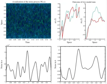
We study the above equations with ν₌10−3 as in Fournier et al. (2007), and withgu=0.01,gb=1. With this choice of parameters, we observe that the random distur-bance to the velocity field u is on the order of 10−5, and that the disturbance to the magnetic fieldb is on the order of 10−1. While the absolute value of the noise onuis quite small, its effect is dramatic because the governing equation is sensitive to perturbations, becauseνis small. An illustration of the noise process and its effect on the solution is given in Fig. 1. The upper left figure shows a realization of the noise processW and illustrates that the noise is smooth in space. The upper right part of Fig. 1 shows two realizations of the solution and, since the two realizations are very different, il-lustrates the need for data assimilation. The lower two panels of Fig. 1 show a typical snapshot of the noise onu(right) and b(left).

We chose the parametersguandgbas large as possible and the parameterνas small as possible without causing instabil-ities in our discretization (see below). For larger values ofgu and smaller values ofν, a more sophisticated discretization is necessary. However, the model itself (independent of the choice of parameters) is a dramatic simplification of more realistic three-dimensional dynamo models, so that the value of studying Eqs. (49) and (50) for larger gb, gu or smaller ν is limited. Our results should be interpreted as “proof of concept,” that implicit sampling can be used to improve the forecast and analysis of the hidden velocity fielduby assim-ilating observations of the magnetic fieldb.

4.1 Discretization of the dynamical equations

We follow Fournier et al. (2007) in the discretization of the dynamical equations, however we present details here to ex-plain how the noise processW comes into play.

For both fields, we use Legendre spectral elements of order N(see e.g. Canuto et al., 2006; Deville et al., 2006), so that

Space Space Space Time Noise in u Noise in b u ( x , T ) b ( x , T ) Space Space

Outcome of two model runs A realization of the noise process W(x,t)

Fig. 1.The noise processW (x, t )and its effects on the solutionu

andb. Upper left: the noise processW (x, t )is plotted as a function ofxandt. Upper right: two realizations of the solution att₌T ₌

0.2. Lower left: a snapshot of the noise onu. Lower right: a snapshot of the noise onb.

u(x, t )₌ N

X

j=0 ˆ

uj(t )ψj(x)= N₋1

X

j=1 ˆ

uj(t )ψj(x),

b(x, t )₌ N

X

j₌0 ˆ

bj(t )ψj(x)= −ψ0(x)+ψN(x)

+ N−1

X

j=1 ˆ

bj(t )ψj(x),

W (x, t )₌ N

X

j=0 ˆ

Wj(t )ψj(x)= N₋1

X

j=1 ˆ

Wj(t )ψj(x),

whereψj are the characteristic Lagrange polynomials of or-derN, centered at thej-th Gauss-Lobatto-Legendre (GLL) nodeξj. We consider the weak form of Eqs. (49) and (50) without integration by parts because the solutions are smooth enough to do so. This weak form requires computation of the second derivatives of the characteristic Lagrange polynomi-als at the nodes, which can be done stably and accurately us-ing recursion formulas. We substitute the series expansions into the weak form of Eqs. (49) and (50) and evaluate the integrals by Gauss-Lobatto-Legendre quadrature

1 Z −1 p(x)dx_∼ N X

j=0

p(ξj)wj,

the set of SDEs M∂tuˆ=M

ˆ

b◦Dbˆ−uˆ◦Duˆ+νD2uˆ+9_xBbˆ+gu∂tWˆ

,

M∂tbˆ=M

ˆ

b_◦Duˆ₋uˆ_◦Dbˆ₊D2bˆ₋9_xBuˆ₊9_xxB ₊gb∂tWˆ

,

where _◦ denotes the Hadamard product ((uˆ_◦bˆ)k= ˆ

ukbˆk), uˆ,bˆ,Wˆ are (N−2)-dimensional column vec-tors whose components are the coefficients in the se-ries expansions of u, b, Wu and Wb, respectively, and where9_xB₌diag (∂xψj(ξ1), . . . , ∂xψj(ξN−1))and9xxB =

(∂xxψ2(ξ1), . . . , ∂xxψN−1(ξN−1))T is a diagonal(N−2)×

(N₋2)matrix and an(N₋2)-dimensional column vector, respectively, which make sure that our approximation sat-isfies the boundary conditions. In the above equations, the (N₋2)×(N₋2)matricesM,DandD2are given by M₌diag((w1, . . . , wN−1)) , Dj,k=∂xψj(ξk),

D2j,k=∂xxψj(ξk).

We apply a first-order implicit-explicit method with time step δ for time discretization and obtain the discrete-time and discrete-space equations

(M₋δνMD2)un+1=

Mun₊δbn_◦Dbn₋un_◦Dun₊9_xBbn₊1Wn_u, (M₋δMD2)bn+1₌

Mbn+δbn◦Dun−un◦Dbn−9_xBun+9xxB

+1Wn_b,

where

1Wu∼N(0, 6u), 1Wb∼N(0, 6b), (56) and

6u=gu2δM

FsCCTFsT +FcCCTFcT

MT, (57)

6b=gb2δM

FsCCTFsT +FcCCTFcT

MT, (58)

C₌diag((α1, . . . , αn)), (59)

Fs =(sin(π ),sin(2π ), . . . ,sin(mπ ))(ξ1, ξ2, . . . , ξm)T, (60) Fc=(cos(π/2),cos(3π/2), . . . ,

cos(mπ/2))(ξ1, ξ2, . . . , ξm)T. (61) For our choice ofαk, βk in Eq. (55), the state covariance matrices 6u and 6b are singular if N >12. To diagonal-ize the state covariances we solve the symmetric eigenvalue problems Parlett (1998)

(M₋δνMD2)vu=6uvuλu, (M₋δMD2)vb=6bvbλb,

and define the linear coordinate transformations

u=Vu(xu,yu)T, b=Vb(xb,yb)T, (62) where the columns of the (N₋2)×(N₋2)-matrices Vu andVbare the eigenvectors ofvu,vb, respectively. The dis-cretization using Legendre spectral elements works in our

200 400 600 800 1000 0.04

0.14 0.2

Number of gridpoints

Logarithm of mean of errors

102 ₁₀3 0.06

0.11 0.16

Logarithm of 1/timestep

Logarithm of mean of errors

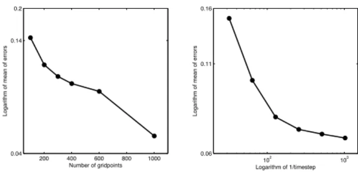
Fig. 2.Convergence of discretization scheme for geomagnetic equa-tions. Left: Convergence in the number of spatial grid-points (log-linear scale). Right: Convergence in the time step (log-log scale).

favor here, because the matrices MandD2 are symmetric so that we can diagonalize the left hand side simultaneously with the state covariance matrix to obtain

xnu+1=fu(xun,ynu,xnb,y n b)+1Wˆ

n u, yn_u+1₌gu(xnu,ynu,xnb,ynb),

xn_b+1₌fb(xnu,ynu,xnb,ynb)+1Wˆnb,

yn_b+1₌gb(xun,ynu,xnb,y n b),

wherefu,fb are 10-dimensional vector functions, gu,gb are((N₋2)−10)-dimensional vector functions and where

ˆ

Wn_{u ∼}N _{0,diag λ}u 1, λ

u 2, . . . , λ

u 10

,

ˆ

Wn_b ∼N0,diagλb₁, λb₂, . . . , λb₁₀.

We test the convergence of our approximation as follows. To assess the convergence in the number of grid-points in space, we define a reference solution usingN₌2000 grid-points and a time step ofδ₌0.002. We compute another ap-proximation of the solution, using the same (discrete) BM as in the reference solution, but with another number of grid-points, sayN₌500. We compute the error att₌T ₌0.2,

ex= ||(u500(x, T )T,b500(x, T )T)−(uRef(x, T )T,bRef(x, T )T)||,

where|| · ||denotes the Euclidean norm, and store it. We re-peat this procedure 500 times and compute the mean of the error norms and scale the result by the mean of the norm of the solution. The results are shown in the left panel of Fig. 2. We observe a straight line, indicating super algebraic con-vergence of the scheme (as is expected from a spectral method).

Similarly, we check the convergence of the ap-proximation in the time step by computing a refer-ence solution with NRef=1000 and δRef=2−12. Using

−1 ₋0.5 0 0.5 1 −1.5

−1 −0.5 0 0.5 1 1.5

−1 ₋0.5 0 0.5 1

−1 −0.5 0 0.5 1 1.5 2 2.5 3

u

(

x,

0) (unobs

e

rve

d va

ri

a

bl

e

s)

b

(

x,

0) (obs

e

rve

d va

ri

a

bl

e

s)

x x

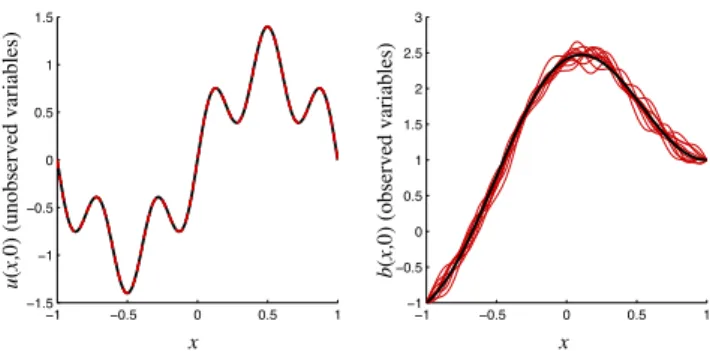
Fig. 3.Uncertainty in the initial state. Left:u(x,0)(unobserved).

Right:b(x,0)(observed). Black: mean. Red: 10 realizations of the

initial state.

(uRef(x, T )T,bRef(x, T )T)_||, and store it. We repeat this procedure 500 times and then compute the mean of these er-ror norms, divided by the mean of the norm of the solution. The results are shown in the right panel of Fig. 2. We ob-serve a first order decay in the error for time steps larger than δ₌0.02 as is expected. The error has converged for time steps smaller thanδ₌0.002, so that a higher resolution in time does not improve the accuracy of the approximation.

Here we are satisfied with an approximation with δ₌ 0.002 andN₌300 grid-points in space as in Fournier et al. (2007). The relatively small number of spatial grid-points is sufficient because the noise is very smooth in space and because the Legendre spectral elements accumulate nodes close to the boundaries and, thus, represent the steep bound-ary layer, characteristic of Eqs. (49)–(50), well even ifN is small (see also Fournier et al., 2007).

4.2 Filtering results

We apply the implicit particle filter with gradient descent minimization and random maps (see algorithm 2 in Sect. 3), the simplified implicit particle filter (see Sect. 2.2) adapted to models with partial noise, a standard EnKF (without lo-calization or inflation), as well as a standard SIR filter to the test problem Eqs. (49)–(50). The numerical model is given by the discretization described in the previous section with a random initial state. The distribution of the initial state is Gaussian with meanu(x,0), b(x,0)as in Eqs. (51)–(52) and with a covariance6u, 6bgiven by Eqs. (57)–(58). In Fig. 3, we illustrate the uncertainty in the initial state and plot 10 re-alizations of the initial state (grey lines) along with its mean (black lines). We observe that the uncertainty inu0is small

compared to the uncertainty inb0.

The data are the values of the magnetic fieldb, measured at kequally spaced locations in [−1,1] and corrupted by noise:

zl=Hbq(l)+sVl, (63)

−1 −0.5 0 0.5 1

−1.2 −1 −0.8 −0.6 −0.4 −0.2 0 0.2 0.4 0.6

−1 −0.5 0 0.5 1

−1 −0.5 0 0.5 1 1.5 2

u

(

x

,T

) (unobs

e

rve

d va

ri

a

bl

e

s)

b

(

x

,T

) (obs

e

rve

d va

ri

a

bl

e

s)

x x

Fig. 4.Outcome of a twin experiment. Black: true stateu(x,0.2)

(left) andb(x,0.2)(right). Red: reconstruction by implicit particle filter with 4 particles.

wheres₌0.001 and whereHis ak_×m-matrix that maps the numerical approximationb(defined at the GLL nodes) to the locations where data is collected. We consider data that are dense in time (r=1) as well as sparse in time (r >1). The data are sparse in space and we consider two cases: (i) we collect the magnetic fieldbat 200 equally spaced locations; and (ii) we collect the magnetic fieldbat 20 equally spaced locations. The velocityuis unobserved and it is of interest to study how the various data assimilation techniques make use of the information inbto update the unobserved variablesu (Fournier et al., 2007, 2010).

To assess the performance of the filters, we ran 100 twin experiments. A twin experiment amounts to (i) drawing a sample from the initial state and running the model forward in time untilt₌T ₌0.2 (one fifth of a magnetic diffusion time Fournier et al., 2007), (ii) collecting the data from this free model run, and (iii) using the data as the input to a fil-ter and reconstructing the state trajectory. Figure 4 shows the result of one twin experiment forr₌4.

For each twin experiment, we calculate and store the error at t₌T ₌0.2 in the velocity, eu= ||u(x, T )− uFilter(x, T )_||, and in the magnetic field, eb= ||b(x, T )− bFilter(x, T )_||. After running the 100 twin experiments, we calculate the mean of the error norms (not the mean error) and the variance of the error norms (not the variance of the error) and scale the results by the mean of the norm ofuand b, respectively. All filters we tested were “untuned”, i.e. we have not adjusted or inserted any free parameters to boost the performance of the filters.

Figure 5 shows the results for the implicit particle filter, the EnKF as well as the SIR filter for 200 measurement locations and forr₌10.

0 500 1000 0.1

0.15 0.2 0.25

0 500 1000

0.01 0.02 0.03 0.04 0.05 0.06 0.07 0.08 0.09 0.1 0.11

E

rror i

n

b

(obs

erve

d va

ri

abl

es

)

E

rror i

n

u

(unobs

erve

d va

ri

abl

es

)

Number of Particles Number of Particles

Implicit filter EnKF SIR filter

Fig. 5.Filtering results for data collected at a high spatial resolution

(200 measurement locations). The errors att=0.2 of the implicit

particle filter (red), EnKF (purple) and SIR filter (green) are plotted as a function of the number of particles. The error bars represent the mean of the errors and mean of the standard deviations of the errors.

The EnKF requires about 500 particles to achieve the accu-racy of the implicit filter with only 4 particles.

In the experiments, we observed that the minimization in implicit particle filtering typically converged after 4–10 steps (depending on r, the gap in time between observations). The convergence criterion was to stop the iteration when the change inFjwas less than 10 %. A more accurate minimiza-tion did not improve the results significantly, so that we were satisfied with a relatively crude estimate of the minimum in exchange for a speed-up of the algorithm. We foundλ by solving Eq. (11) with Newton’s method usingλ0₌0 as ini-tial guess and observed that it converged after about eight steps. The convergence criterion was to stop the iteration if

|F (λ)₋φ₋ρ_{| ≤}10−3, because the accurate solution of this scalar equation is numerically inexpensive. We resampled us-ing algorithm 2 in Arulampalam et al. (2002), if the effective sample sizeMEffin Eq. (19) divided by the number of

parti-clesMis less than 90 % of the number of particles.

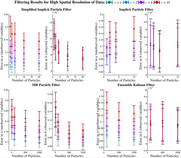
To further investigate the performance of the filters, we run more numerical experiments and vary the availability of the data in time, as well as the number of particles. Figure 6 shows the results for the implicit particle filter, the simplified implicit particle filter, the EnKF and the SIR filter for 200 measurement locations and forr₌1,2,4,10.

We observe from Fig. 6, that the error statistics of the im-plicit particle filter have converged, so that there is no signif-icant improvement when we increase the number of particles to more than 10. In fact, the numerical experiments suggest that no more than 4 particles are required here. Independent of the gap between the observations in time, we observe an error of less than 1 % in the observed variableb. The error in

the unobserved variableu, however, depends strongly on the gap between observations and, for a large gap, is about 15 %. The reconstructions of the observed variables by the sim-plified implicit particle filter are rather insensitive to the availability of data in time and, with 20 particles, the sim-plified filter gives an error in the observed quantitybof less than 1 %. The errors in the unobserved quantity u depend strongly on the gap between the observations and can be as large as 15 %. The error statistics in Fig. 6 have converged and only minor improvements can be expected if the number of particles is increased to more than 20.

The SIR filter required significantly more particles, than the implicit filter or simplified implicit filter. Independent of the gap between observations, the errors and their variances are larger than for the implicit and simplified implicit filter, even if the number of particles for SIR is set to 1000. The EnKF performs well and, for about 500 particles, gives re-sults that are comparable to those of the implicit particle fil-ter. The EnKF may give similarly accurate results at a smaller number of particles if localization and inflation techniques are implemented.

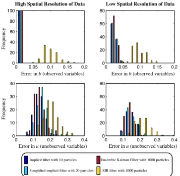
The errors in the reconstructions of the various filters are not Gaussian, so that an assessment of the errors based on the first two moments is incomplete. In the two panels on the right of Fig. 7, we show histograms of the errors of the implicit filter (10 particles), simplified implicit filter (20 par-ticles), EnKF (1000 particles) and SIR filter (1000 particles) forr₌10 model steps between observations.

We observe that the errors of the implicit filter, simplified implicit filter and EnKF are centered to the left of the di-agrams (at around 10 % in the unobserved quantity u and about 1 % for the observed quantityb) and show a consider-ably smaller spread than the errors of the SIR filter, which are centered at much larger errors (20 % in the unobserved quan-tityuand about 9 % for the observed quantityb). A closer look at the distribution of the errors thus confirms our con-clusions we have drawn from an analysis based on the first two moments.

We further assess the performance of the filters by con-sidering their effective sample size (19), which measures the quality of the particles ensemble Doucet et al. (2001). A large effective sample size indicates a good ensemble, i.e. the sam-ples are independent and each of them contributes signifi-cantly to the approximation of the conditional mean; a small effective sample size indicates a “bad ensemble”, i.e. most of the samples carry only a small weight. We computed the effective sample size for the implicit particle filter, the sim-plified implicit particle filter and the SIR filter after each as-similation, and compute the average after each of 100 twin experiments. In Table 1, we show the average effective sam-ple size (averaged over all 100 twin experiments and scaled by the number of particles) for a gap ofr₌10 model steps between observations.

0 500 1000

0.1 0.15 0.2 0.25 0.3 0.35

0 500 1000

0.06 0.08 0.1 0.12 0.14 0.16 0.18

Implicit Particle Filter

SIR Particle Filter Ensemble Kalman Filter

Simplified Implicit Particle Filter

Number of Particles Number of Particles Number of Particles Number of Particles

Number of Particles Number of Particles Number of Particles Number of Particles

Filtering Results for High Spatial Resolution of Data: r = 1 r = 2 r = 4 r = 10

Error in

b

(observed variables)

Error in

u

(unobserved variables)

Error in

b

(observed variables)

Error in

u

(unobserved variables)

Error in

b

(observed variables)

Error in

u

(unobserved variables)

Error in

b

(observed variables)

Error in

u

(unobserved variables)

Fig. 6.Filtering results for data collected at a high spatial resolution (200 measurement locations). The errors att₌0.2 of the simplified implicit particle filter (upper left), implicit particle filter (upper right), SIR filter (lower left) and EnKF (lower right) are plotted as a function of the number of particles and for different gaps between observations in time. The error bars represent the mean of the errors and mean of the standard deviations of the errors.

Table 1.Effective sample size of the simplified implicit filter, the implicit filter and the SIR filter.

Simplified Implicit SIR

implicit filter filter filter

MEff/M 0.20 0.19 0.02

of the SIR filter. This result indicates that the particles of the implicit filter are indeed focussed towards the high probabil-ity region of the target pdf.

Next, we decrease the spatial resolution of the data to 20 measurement locations and show filtering results from 100 twin experiments in Fig. 8.

The results are qualitatively similar to those obtained at a high spatial resolution of 200 data points per observation. The two panels on the right of Fig. 7, show histograms of the errors of the implicit filter (10 particles), simplified im-plicit filter (20 particles), EnKF (1000 particles) and SIR

filter (1000 particles) for r₌10 model steps between ob-servations. Again, the results are qualitatively similar to the results we obtained at a higher spatial resolution of the data. We observe for the implicit particle filter that the errors in the unobserved quantity are insensitive to the spatial resolu-tion of the data, while the errors in the observed quantity are determined by the spatial resolution of the data and are rather insensitive to the temporal resolution of the data. These ob-servations are in line with those reported in connection with a strong 4-D-Var algorithm in Fournier et al. (2007). All other filters we have tried show a dependence of the errors in the observed quantity on the temporal resolution of the data.

0 0.05 0.1 0.15 0.2 0

20 40 60 80 100

0 0.1 0.2 0.3 0.4 0

10 20 30 40

0 0.05 0.1 0.15 0.2 0

20 40 60 80

0 0.1 0.2 0.3 0.4 0

20 40 60 80

Error in u (unobserved variables) Error in u (unobserved variables) Error in b (observed variables) Error in b (observed variables)

F

re

que

nc

y

F

re

que

nc

y

Implicit filter with 10 particles

Simplified implicit filter with 20 particles

Ensemble Kalman Filter with 1000 particles

SIR filter with 1000 particles

High Spatial Resolution of Data Low Spatial Resolution of Data

Fig. 7.Histogram of errors att=0.2 of the implicit filter, simplified implicit filter, EnKF and SIR filter. Left: data are available at a high

spatial resolution (200 measurement locations) and everyr=10

model steps. Right: data are available at a low spatial resolution

(20 measurement locations) and everyr=10 model steps.

within the high probability region by solving Eq. (11). Be-cause the implicit filter focusses attention on regions of high probability, only a few samples are required for a good accu-racy of the state estimate (the conditional mean). The infor-mation in the observations of the magnetic fieldbpropagates to the filtered updates of the unobserved velocityuvia the nonlinear coupling in Eqs. (49)–(50).

The EnKF on the other hand uses the data only at times when an observation is available. The state estimates at all other times are generated by the model alone. Moreover, the nonlinearity, and thus the coupling of observed and unob-served quantities, is represented only in the approximation of the state covariance matrix, so that the information in the data propagates slowly to the unobserved variables. The sit-uation is very similar for the simplified implicit filter.

The SIR filter requires far more particles than the implicit filter because it samples the low probability region of the tar-get pdf with a high probability. The reason is that the overlap of the pdf generated by the model alone and the target pdf be-comes smaller and smaller as the data bebe-comes sparser and sparser in time. For that reason, the SIR filter must generate far more samples to at least produce a few samples that are likely with respect to the observations. Moreover, the data is only used to weigh samples that are generated by the model alone; it does not use the nonlinear coupling between ob-served and unobob-served quantities, so that the information in

the data propagates very slowly from the observed to the un-observed quantities.

In summary, we observe that the implicit particle filter yields the lowest errors with a small number of particles for all examples we considered, and performs well and reliably in this application. The SIR and simplified implicit particle filters can reach the accuracy of the implicit particle filter, at the expense that the number of particles is increased signifi-cantly. The very small number of particles required for a very high accuracy make the implicit filter the most efficient fil-ter for this problem. Note that the partial noise works in our favor here, because the dimension of the space the implicit filter operates in is 20, rather than the state dimension 600.

Finally, we wish to compare our results with those in Fournier et al. (2007), where a strong constraint 4-D-Var al-gorithm was applied to the deterministic version of the test problem. Fournier and his colleagues used “perfect data,” i.e. the observations were not corrupted by noise, and ap-plied a conjugate-gradient algorithm to minimize the 4-D-Var cost function. The iterative minimization was stopped af-ter 5000 iaf-terations. With 20 observations in space and a gap ofr₌5 model steps between observations, an error of about 1.2 % inuand 4.7 % inbwas achieved. With the implicit fil-ter, we can get to a similar accuracy at the same spatial reso-lution of the data, but with a larger gap ofr₌10 model steps between observations. However, the 4-D-Var approach can handle larger uncertainties and errors in the velocity field. The reason is that the initial conditions are assumed to be known (at least roughly) when we assimilate data sequen-tially. This assumption is of course not valid in “real” geo-magnetic data assimilation (the velocity field is unknown), however a strong 4-D-Var calculation can be used to obtain approximate and uncertain initial conditions to then start as-similating new data with a filter. The implicit particle filter then reduces the memory requirements because it operates in the 20-dimensional subspace of the forced variables and assimilates the data sequentially. Each minimization is thus not as costly as a 600-dimensional strong constraint 4-D-Var minimization. Alternatively, one could extend the implicit particle filter presented here to include the initial conditions as variables of theFjs. This set up would allow for larger uncertainties in the initial conditions than what we presented here.

5 Conclusions