www.geosci-model-dev.net/8/2829/2015/ doi:10.5194/gmd-8-2829-2015
© Author(s) 2015. CC Attribution 3.0 License.
A new ensemble-based consistency test for the Community Earth
System Model (pyCECT v1.0)
A. H. Baker, D. M. Hammerling, M. N. Levy, H. Xu, J. M. Dennis, B. E. Eaton, J. Edwards, C. Hannay, S. A. Mickelson, R. B. Neale, D. Nychka, J. Shollenberger, J. Tribbia, M. Vertenstein, and D. Williamson The National Center for Atmospheric Research, Boulder, CO, USA
Correspondence to: A. H. Baker ([email protected])
Received: 15 April 2015 – Published in Geosci. Model Dev. Discuss.: 8 May 2015 Revised: 22 August 2015 – Accepted: 24 August 2015 – Published: 9 September 2015
Abstract. Climate simulation codes, such as the Community Earth System Model (CESM), are especially complex and continually evolving. Their ongoing state of development re-quires frequent software verification in the form of quality assurance to both preserve the quality of the code and instill model confidence. To formalize and simplify this previously subjective and computationally expensive aspect of the ver-ification process, we have developed a new tool for evalu-ating climate consistency. Because an ensemble of simula-tions allows us to gauge the natural variability of the model’s climate, our new tool uses an ensemble approach for con-sistency testing. In particular, an ensemble of CESM climate runs is created, from which we obtain a statistical distribution that can be used to determine whether a new climate run is statistically distinguishable from the original ensemble. The CESM ensemble consistency test, referred to as CESM-ECT, is objective in nature and accessible to CESM developers and users. The tool has proven its utility in detecting errors in software and hardware environments and providing rapid feedback to model developers.
1 Introduction
The Community Earth System Model (CESM) is a state-of-the-art, fully coupled, global climate model whose develop-ment is centered at the National Center for Atmospheric Re-search (NCAR) (Hurrell et al., 2013). Earth’s global climate is complex, and CESM is widely used by scientists around the world to further our understanding of the future, present and past states of the climate system. For large simulation models such as CESM, verification and validation are
exam-ple, porting the CESM code to a new machine architecture results in non-BFB model output, and the current approach is as follows. First, a climate simulation of several hundred years (typically 400) is run on the new machine. Next, data from the new simulation is analyzed and compared to data from the same simulation run on a “trusted” machine, and, lastly, all results are given to a senior climate scientist for ap-proval. This informal process is not overly rigorous and re-lies largely on subjective evaluations. Further, running a sim-ulation for hundreds of years is resource intensive, and this expense is exacerbated as the model grows larger and more complicated. Clearly a more rapid, objective, and accessible solution is needed, particularly because a port of CESM to a new machine is just one example of a non-BFB change that requires quality assurance testing. Other common situations that can lead to non-BFB results include experiments with new compiler versions or optimizations, code modifications that are not expected to be climate-changing, and many new exascale-computing technologies. The lack of a straightfor-ward metric for accessing the quality of the simulation out-put has limited the ability of CESM users and developers to introduce potential code modifications and performance im-provements that result in non-BFB reproducibility. The need for a more quantitative solution for ensuring code quality prompted our development of a new tool for assessing the impact of non-BFB changes in CESM. While verification al-ways involves some degree of subjectivity and one cannot absolutely prove correctness (Carson II, 2002; Oberkamf and Roy, 2010), we aim to facilitate the detection of hardware, software, or human errors introduced into the simulation.
The quality assurance component of code verification im-plies that a degree of consistency must exist (Oberkamf and Roy, 2010). Our new method evaluates climate consistency in CESM via an ensemble-based approach that simplifies and formalizes the quality assurance piece of the current verifica-tion process. In particular, the goal of our new CESM en-semble consistency test tool, referred to as CESM-ECT, is to easily determine whether or not a change in a CESM simula-tion is statistically significant. The ability of this simple tool to quickly assess changes in simulation output is a significant step forward in the pursuit of more qualitative metrics for the climate modeling community. The tool has already proven invaluable in terms of providing more feedback to model de-velopers and increasing confidence in new CESM releases. Note that we do not discuss verification of the underlying numerical model in this work, which is considered at other stages in the development of individual CESM components. Further, we do not address model validation, but mention that it is primarily conducted via hindcasts and comparisons to real world data, e.g., the Intergovernmental Panel on Climate Change Data Distribution Centre has a large collection of ob-served data (IPCC Data Collection Centre, 2015).
This paper is organized as follows. We give additional background information in Sect. 2. We describe the new CESM-ECT tool in Sect. 3. In Sect. 4, we provide results
from experiments with CESM-ECT, and in Sect. 5 we give examples of the utility of the new tool in practice. Finally, we give concluding remarks and discuss future work in Sect. 6.
2 Background
Climate science has a strong computational component, and the climate codes used in this discipline are typically com-plex and large in size (e.g., Easterbrook et al., 2011; Pipitone and Easterbrook, 2012), making the thorough evaluation of climate model software quite challenging (Clune and Rood, 2011). In particular, the CESM code base, which has been developed over the last 20 years, currently contains about one and a half million lines of code. CESM consists of multi-ple geophysical component models of the atmosphere, ocean, land, sea ice, land ice, and rivers. These components can all run on different grid resolutions, exchanging boundary data with each other through a central coupler. Because CESM supports a variety of spatial resolutions and timescales, sim-ulations can be run on both state-of-the-art supercomputers as well as on an individual scientist’s laptop. The myriad of model configurations available to the user contribute to the difficulty of exhaustive software testing (Clune and Rood, 2011; Pipitone and Easterbrook, 2012). A particularly fas-cinating and in-depth description of the challenges of sci-entific software in general, and climate modeling software in particular, can be found in Easterbrook and Johns (2009). Furthermore, the societal importance of better understanding Earth’s climate is such that every effort must be made to ver-ify climate codes as well as possible (e.g., Easterbrook et al., 2011).
of simulation output (Easterbrook and Johns, 2009). Visu-alizations of model output are commonly examined by cli-mate scientists, and achieving BFB identical results has been quite important to the climate community (Easterbrook and Johns, 2009; Pipitone and Easterbrook, 2012). If changes in the source code or software and hardware environment yield BFB results to the previous version, then this verification step is trivial. However, depending on the nature of the change, achieving BFB results from one run to the next is not al-ways possible. For example, in the context of porting the code to a new machine architecture, machine-rounding level changes can propagate rapidly in a climate model (Rosinski and Williamson, 1997). In fact, changes in hardware, soft-ware stack, compiler version, and CESM source code can all cause round-off level or larger changes in the model simula-tion results, and the emergence of some heterogeneous com-puting technologies inhibit BFB reproducibility as well.
Some of the difficulties caused by differences due to trun-cation and rounding in climate codes that result in non-BFB simulation data are discussed in Clune and Rood (2011). In particular, the authors cite the need for determining ac-ceptable error tolerances and the concern that seemingly mi-nor software changes can result in a different climate if the simulation is not run for a sufficient amount of time. The work in Rosinski and Williamson (1997) is also of interest and aims to determine the validity of a simulation when mi-grating to a new architecture. They minimize the computa-tional expense of a long run by setting tolerances for round-ing accumulation growth based on the growth of a small per-turbation in the atmospheric temperature after several days. However, this test is no longer applicable to the atmospheric component of CESM, called the Community Atmosphere Model (CAM), because the parameterizations in CAM5 are ill-conditioned in the sense that small perturbations in the in-put produce large perturbations in the outin-put. The result is that the tolerances for rounding accumulation growth are ex-ceeded within the first few time steps. Our work builds on this idea of gauging the effects of a small temperature pertur-bation on the simulation, though improvements in software and hardware allow us to extend the simulation duration well beyond several days. Further, by looking only at climate sig-nals, we relax the restriction on how the parameterizations respond.
3 A new method for evaluating consistency
In this section, we present and discuss a new ensemble con-sistency test for CESM, called CESM-ECT. We first give a broad overview, followed by more details in the subsequent subsections. As noted, CESM’s evolving code base and the demand to run on new machine architectures often result in data that are not BFB identical to previous data. Therefore, our new tool for CESM must determine whether or not the new configuration (e.g., code generated with a different
com-piler option, on a new architecture, or after a non-climate changing code modification) should be accepted. For our pur-poses, we accept the new configuration if its output data is statistically indistinguishable from the original data, where the original data refers to data generated on a trusted ma-chine with an accepted version of the software stack. Our tool must
– determine whether or not data from a new configuration is consistent with the original data
– indicate the level of confidence in its determination (e.g., false positive rate)
– be user-friendly in terms of ease of use and minimal computational requirements for the end-user.
Note that this new tool takes a coarse-grained approach to detecting statistical differences. Its purpose is not to isolate the source of an inconsistency but rather to indicate the likeli-hood that one exists. To this end, the CESM-ECT tool works as follows. The first step requires the creation of an ensemble of simulations in an accepted environment representing the original data. The second step uses the ensemble data to de-termine the statistical distributions that describe the original data. Next, several simulations representing the new data are obtained. And, finally, a determination is made as to whether the new data are statistically similar to the original ensemble data.
3.1 Preliminaries
CESM data are written to “history” files in time slices in NetCDF format for post-processing analysis. Data in his-tory files are of single precision (by default). For this initial work, we focus on history data from the CAM component in CESM, which is actively developed at NCAR. We chose to begin with CAM because the timescales for changes propa-gating through the atmosphere are relatively short compared to the longer timescales of other components, such as the ocean, ice, or land models. Further, the set of CAM global output variables is diverse, and the default number for our CESM configuration (detailed in the next section) is on the order of 130. An error in CAM would certainly affect the other model components in fully coupled CESM situations; however, we cannot assume that CAM data passing CESM-ECT implies that the remaining components would also pass. Data from other components (e.g., ocean, ice, and land) will be addressed in future work, though we give an example in Sect. 5 of detecting errors stemming from the ice component with CESM-ECT.
3.2 An ensemble method
that the difference be less than the natural variability of the climate system makes sense intuitively and is along the lines of Condition 2 in Rosinski and Williamson (1997). However, characterizing the natural variability is difficult with a single run of the original simulation. Therefore, we extend the sam-pling of the original data to an ensemble from which we can obtain a statistical distribution. An ensemble refers to a col-lection of multiple realizations of the same model simulation, generated to represent possible states of the system (e.g., Dai et al., 2001). Generally, small perturbations in the initial con-ditions are used to generate the ensemble members, and the idea is to characterize the climate system with a representa-tive distribution (as opposed to a single run). Ensembles are commonly used in climate modeling and weather forecasting (see, e.g., Dai et al., 2001; Zhu and Toth, 2008; von Storch and Zwiers, 2013; Zhu, 2005; Sansom et al., 2013) to en-hance model confidence, indicate uncertainly, and improve predictions. For example, the ensemble in Kay et al. (2015) was created by small perturbations to the initial temperature condition in CAM and is being used to study internal climate variability.
We generate our ensemble for CESM-ECT by running simulations that differ only in a random perturbation of the initial atmospheric temperature field ofO(10−14). These per-turbations grow to the size of NWP (numerical weather pre-diction) analysis errors in a few hours. Each simulation is 1 year in length, which is short enough to be computationally reasonable, yet of sufficient length to allow the effects of the perturbation to propagate through the system. A perturbation of this size should not be climate-changing and, while 1 year is inadequate to establish a climate, it is sufficient for gen-erating the statistical distribution that we need. In particular, while the trajectories of the ensemble members will rapidly diverge due to the chaotic nonlinearity of the model, the sta-tistical properties of the ensemble members are expected to be the same. Determining the appropriate number of ensem-ble members requires a balance between computational and storage costs and the quality of the distribution. The lower bound on the size is constrained by our use of principal com-ponent analysis (PCA), which is described in the next subsec-tion. PCA requires that the number of ensemble members be larger than the number of CAM variables. We chose an ini-tial ensemble size, denoted byNens, of 151 for CESM-ECT.
At this size, the coefficient of variation for each CAM vari-able is well under 5 %, save for two varivari-ables that are known to have large distributions across the ensemble (meridional surface stress and meridional flux of zonal momentum). The cost to generate the ensemble is reasonable because allNens,
members can be run in parallel, resulting in a much faster turn around time than for a single multi-century run (a sin-gle 1-year simulation can run in a couple hours on less than a thousand cores). Note that, as explained further in Sect. 3.5, an ensemble is only generated for the control and not for the code to be tested. Hence, the ensemble creation does not im-pact the CESM-ECT user.
In summary, the CESM-ECT ensemble consists of
Nens=151 1-year climate simulations, denoted by E=
{E1, E2, . . ., ENens} and is produced on a trusted machine with an accepted version, model, and configuration of the cli-mate code. The data for these 1-year ensemble runs consists of annual temporal averages at each grid point for the se-lected grid resolution for allNvar variables, which are either
two- or three-dimensional. Retaining only the annual tem-poral averages for each variable helps to reduce the cost of storing the ensemble simulation output and has proved suffi-cient for our purposes. We denote the data set for a variable
X asX= {x1, x2, . . ., xNX}, where xi is a scalar that repre-sents the annual (temporal) average at grid pointiandNXis the total number of grid points inX(determined by whether
Xis a 2-D or 3-D variable).
3.3 Characterizing the ensemble data
The next stage in our process is the creation of the statistical distributions that describe the ensemble data. In particular, information collected from the ensemble simulations helps to characterize the internal variability of the climate model system. Results from new simulations (resulting from a non-BFB change) can then be compared to the ensemble distribu-tion to determine consistency.
First, based on the ensemble simulation output, CESM-ECT calculates the global area-weighted mean distributions, providing climate scientists with an indication of the aver-age state and variability across the control ensemble for each variable. However, determining whether or not the climate in the new run is consistent with the ensemble data based on the number of variables that fall within the global mean distribution (or other specified tolerance) is difficult with-out a linearly independent set of variables. For the CESM 1.3.x series, 134 variables are output by default for CAM. We exclude several redundant variables as well as those with zero variance across the ensemble (e.g., specified variables common to all ensemble runs) from our analysis, resulting in
Nvar=120 variables total (see Appendix A for more detail).
analysis, particularly when there are large number of vari-ables.
CESM-ECT applies PCA-based testing to the global mean data, and the implementation of the PCA-based testing strat-egy into our tool entails the following steps. First, for each ensemble memberm, the global area-weighted mean is cal-culated for each variableX across all grid pointsiand de-noted by Xm. Next, we standardize the Nvar×Nens matrix
containing the global means for each variable in each en-semble member and denote the result by Vgm. Note that
Nvar=120 andNvar<Nens. Standardization of the data
in-volves subtracting the ensemble mean and dividing by the ensemble standard deviation for each variable and is impor-tant because the CAM variables have vastly different units and magnitudes. Next, we calculate the transformation ma-trix, or “loadings”, that project the variable space Vgm into
principal component (PC) space. Loading matrix Pgmhas the
sizeNvar×Nvar and corresponds to the eigenvector
decom-position of the covariance of Vgm, ordered such that the first
PC corresponds to the largest eigenvalue and decreasing from there. Finally, we apply the transformation to Vgmto obtain
the PC scores, Sgm, for our ensemble:
Sgm=PgmTVgm. (1)
Now instead of using a distribution of variable global means to represent our ensemble, theNvar×Nensmatrix Sgmforms
a distribution of PC scores that represents the variance struc-ture in the data. These scores have a mean of zero, so we only need to calculate the standard deviation of the ensemble scores in Sgm, which we denote byσSgm. To summarize, this first stage computes the following data:
– Nvar×Nensglobal means
– Nvarmeans of ensemble global mean values (µVgm) – Nvarstandard deviations of ensemble global mean
val-ues (σVgm)
– Nvar×Nvarloadings (Pgm)
– Nvar standard deviations of ensemble global mean
scores (σSgm),
which are written to the CESM-ECT ensemble summary file. This summary file (in NetCDF format) is generated for each CESM software tag on the Yellowstone machine at NCAR with the default compiler options (more details follow in Sect. 3.5).
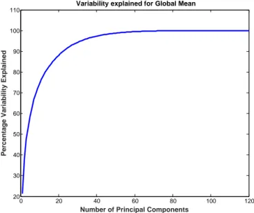
The distribution of global mean scores from the ensemble, represented by the standard deviations inσSgm, can be used to evaluate data from a new simulation. Note that most of the variance in the climate data is now largely represented by a few PCs. In fact, the coefficients on the first PC explain about 21 % of the variance and the coefficients on the second explain about 17 % of the variance, as shown in Figure 1.
0 20 40 60 80 100 120
20 30 40 50 60 70 80 90 100 110
Number of Principal Components
Percentage Variability Explained
Variability explained for Global Mean
Figure 1. Percentage of variability explained for global mean by
component scores.
3.4 Determining a pass or fail
The last step in the CESM-ECT procedure evaluates whether the new output data that has resulted from the non-BFB change is statistically distinguishable from the original en-semble data, as represented by the enen-semble summary file. For simplicity of discussion, assume that we want to evaluate whether the results obtained on a new machine, Yosemite, are consistent (i.e., not statistically distinguishable) with those on Yellowstone. To do this, we collect data from a small num-ber (Nnew) of randomly selected ensemble runs on Yosemite.
Variables in the new data sets are denoted byXe, whereXe= {ex1,ex2, . . .,exNX}. The CESM-ECT tool then decides whether or not the output data from simulations on Yosemite are con-sistent with the ensemble data and issues an overall pass or fail result.
CESM-ECT determines an overall pass or fail in the fol-lowing manner. First, the weighted area global means for each variable Xe in all Nnew runs are calculated, Xfk (k=
1:Nnew). These new variable means are then standardized
using the mean and standard deviations of the control en-semble given in the summary file (µVgm andσVgm). Second, the standardized means are converted to scores via the load-ing matrix Pgmfrom the summary file. Next, we determine
NrunFails≤Nnew. If at leastNpcFailsPCs fail at leastNrunFails
runs, then CESM-ECT returns an overall “failure”.
In typical applications, PC scores with small contributions to the total variability are neglected, and one only examines the firstNPCcomponents in an analysis. However, in the
con-text of detecting errors in the hardware or software system, the PCs that are responsible for the most variability are not necessarily the most relevant. Recalling that each PC is a lin-ear combination of all of the variables, we use a value for
NPCthat both contains sufficient information to detect errors
in any of the variables and allows for a low false positive rate. Our extensive testing indicates thatNPC=50 is sufficient to
detect errors for our particular setup.
The parametersmσ,Nnew,NpcFails, andNrunFails are also
chosen to obtain a desired false positive rate. We performed an empirical simulation study and tested a variety of com-binations of parameters. We found that choosing mσ=2 (which corresponds to the 95 % confidence level),Nnew=3,
NpcFails=3, andNrunFails=2 yields our desired false
posi-tive rate of 0.5 %. To summarize, we run three simulations on Yosemite, and if at least three of the same PCs fail for at least two of these runs, then CESM-ECT issues a “fail-ure”. We intentionally err on the conservative side by choos-ing a low false positive rate, hedgchoos-ing against the possibility that our ensemble may not be capturing all the variability that we want to accept. Also note that while perturbing the initial temperature condition is a common method of ensemble cre-ation for studying climate variability, other possibilities exist, and we are currently conducting further research on the ini-tial ensemble composition and its representation of the range of variability, particularly in regard to compilers and machine modifications.
3.5 CESM-ECT software tools
Finally, we further discuss the software tools needed to test for ensemble consistency that are included in the CESM pub-lic releases (see Sect. 6 for details). Generating the ensem-ble simulation data by setting up and running theNens=151
1-year simulations is the most compute-intensive step in this ensemble consistency-testing process. The CESM Software Engineering group generates ensembles as needed. For ex-ample, generating new ensemble simulation data is now rou-tine when a CESM software tag is created that contains a sci-entific change known to alter the climate from the previ-ous tag. (The frequency of such tag creation varies, but is several times a year on average.) While the utility used to generate the ensemble runs is included in CESM releases, the typical end-user does not need to generate their own en-sembles. Note that our consistency-testing methodology can be extended to other simulation models and, in that case, an application-specific tool to facilitate the generation of Nens
simulations would be needed for the new application. Whenever a new ensemble of simulations is generated, a summary file (as described in Sect. 3.3) must be created for
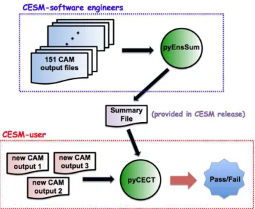
the ensemble. The ensemble summary utility (pyEnsSum), written in parallel Python, creates a NetCDF summary for any specified number (Nens) of output files. This step requires
far less time than it takes to run the simulations themselves. As an example, generating the summary file for 151 ensem-ble members on 42 cores of Yellowstone takes about 20 min (we chose the number of cores to be equal to the number of 3-D variables). Note that the summary creation takes less than a minute when we only compute the information needed for the PCA test (i.e., exclude optional calculations of quan-tities such as the root-mean-squared Z scores). Each CESM software tag now includes the corresponding ensemble sum-mary file. Including the sumsum-mary file in the CESM releases facilitates tracking data changes in the software life cycle and enables CESM users to run CESM-ECT without creating an ensemble of simulations themselves. Note that the storage cost for a single summary file is minor compared to the cost of storing the simulation output for the entire ensemble.
In addition to an ensemble summary file, our Python tool CESM-ECT (pyCECT) requires Nnew=3 1-year
simula-tions from the configuration that is to be tested. For a CESM developer or advanced user, this may mean using a develop-ment version of code with a modification that needs to be tested. For a basic CESM-user, this may mean verifying that the user’s installation of CESM on their personal machine is acceptable. In either case, a simple shell script that cre-ates 1-year CESM run cases (with random initial perturba-tions) for this purpose is also included in CESM releases, though advanced users can certainly generate more custom simulations if desired. Regardless, after theNnewsimulations
have been completed, pyCECT determines whether results from the new configuration are consistent with the original ensemble data based on the supplied new CAM output files and specified ensemble summary file. Then pyCECT reports whether of not the new configuration has passed or failed the consistency test, as well as which PCs in particular have passed or failed each of the Nnew simulations contributing
to the overall pass/fail rating. In addition, the user may as-sign values to the pyCECT parametersmσ,Nnew,NpcFails,
NrunFails, andNPCvia input parameters if the defaults are not
desired.
For clarity, Fig. 2 illustrates the workflow for the CESM-ECT process. The two Python tools are indicated by green circles. The dashed blue box delineates the work done pre-release by the CESM-software engineers. If a CESM user wants to evaluate a new configuration, the user simply exe-cutes the steps in the dashed red box.
4 Experimental studies
can-Figure 2. Graphic of CESM-ECT software tools (circles) and
work-flow.
not (ever) be absolutely sure that this distribution is “correct” in terms of capturing all signatures that lead to the same cli-mate. Our confidence in this initial ensemble distribution is due, in part, to the vast experience and intuition of the CESM climate scientists. However, we gain further confidence with a series of tests of trusted scenarios (i.e., scenarios that we expect to produce the same climate) and verify that those sce-narios pass the CESM-ECT. Similarly, we sample scesce-narios that we expect to be climate-changing and should, therefore, fail.
4.1 Preliminaries
We obtained the results in this work from the 1.3 release se-ries of CESM, using a present-day F compset (active atmo-sphere and land, data ocean, and prescribed ice concentra-tion) and CAM5 physics. We examine 120 (out of a pos-sible 134) variables from the CAM history files, as redun-dant variables and those with no variance are excluded. Of the 120 variables, 78 are two-dimensional and 42 are three-dimensional variables. This spectral-element version of CAM uses a ne=30 resolution (“ne” refers to the number of elements on the edge of the cube), which corresponds ap-proximately to a 1◦global grid containing a total of 48 602 horizontal grid points and 30 vertical levels. Unless oth-erwise noted, simulations were run with 900 MPI (Mes-sage Passing Interface) tasks and two OpenMP (Open Multi-Processing) threads per task on the Yellowstone machine at NCAR. The default compiler on Yellowstone for our CESM version is Intel 13.1.2 with−O2 optimization.
4.2 Non-climate changing modifications
First we look at modifications that lead to non-BFB results but are not expected to be climate-changing. Such modifi-cations include equivalent code formulations that result in the reordering in floating-point arithmetic operations, thus affecting the rounding error. Two common CESM configura-tions that induce reordering in arithmetic operaconfigura-tions include removing thread-level parallelism from the model and cer-tain compiler changes. We expect that the following tests on Yellowstone will not be climate-changing and, thus, will be consistent with our initial ensemble distribution.
– NO-OPT: changing the Intel compiler flag to remove optimization (−O0).
– INTEL-15: changing the Intel compiler version to 15.0.0.
– NO-THRD: compiling CAM without threading (MPI-only).
– PGI: using the CESM-supported PGI compiler (13.0). – GNU: using the CESM-supported GNU compiler
(4.8.0).
These five scenarios differ from the control run used to gen-erate the ensemble only in the single aspect listed above. We first generateNnew=3 simulations on Yellowstone
cor-responding to each test scenario, where each simulation is given a perturbation selected at random from the perturba-tions used to create the initial ensemble. Table 2 lists the pass/fail result from pyCECT and indicates that none of these modifications caused a failure. Recall that our criteria for failure in pyCECT is that at least three PCs must fail at least two of the runs. Table 2 shows that at most two PCs failed two runs for these particular test scenarios.
4.3 CAM climate-changing parameter modifications CESM-ECT also must successfully detect changes to the simulation results that are known to be climate-changing and return a failure. To this end, climate scientists provided a list of CAM input parameters thought to affect the climate in a non-trivial manner. Parameter values were modified to be those intended for use with different CAM configurations (e.g., high-resolution and finite volume). We ran the follow-ing test scenarios which were identical to the default ensem-ble case with the exception of the noted CAM parameter change (the name of the CAM parameter is indicated in ital-ics and its original default value in parenthesis).
– DUST: dust emissions; dust_emis_fact = 0.45 (0.55). – FACTB: wet deposition of aerosols convection factor;
– FACTIC: wet deposition of aerosols convection factor; sol_factic_interstitial = 1.0 (0.4).
– RH-MIN-LOW: min. relative humidity for low clouds; cldfrc_rhminl = 0.85 (0.8975).
– RH-MIN-HIGH: min. relative humidity for high clouds; cldfrc_rhminh = 0.9 (0.8).
– CLDFRC-DP: deep convection cloud fraction; cld-frc_dp1 = 0.14 (0.10).
– UW-SH: penetrative entrainment efficiency – shallow; uwschu_rpen = 10.0 (5.0).
– CONV-LND: autoconversion over land in deep convec-tion; zmconv_c0_lnd = 0.0035 (0.0059).
– CONV-OCN: autoconversion over ocean in deep con-vection; zmconv_c0_ocn = 0.0035 (0.045).
– NU-P: hyperviscosity for layer thickness (vertical la-grangian dynamics); nu_p = 1.0×10⁻¹⁴(1.0×10⁻¹⁵). – NU: dynamics hyperviscosity (horizontal diffusion); nu
= 9.0×10⁻¹⁴(1.0×10⁻¹⁵).
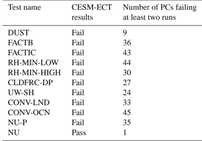
From Table 1, most of these tests fail by a lot more than three PCs, indicating that the new simulation data is quite different from the original ensemble data. However, contrary to our initial expectations, one scenario was found to be consistent and passed. Upon further investigation, the change caused by NU likely did affect some aspects of the climate in a way that would not be detected by the test. The issue is that modifica-tions to NU cause changes at the small scales (but not to the mean of the field the diffusion is applied to) and generally af-fect the extremes of climate variables (such as precipitation). Because CESM-ECT looks at variable annual global means, the “pass” result is not entirely surprising as errors in small-scale behavior are unlikely to be detected in a yearly global mean. Developing the capability to detect the influence of small-scale events is a subject for future work.
4.4 Modifications with unknown outcome
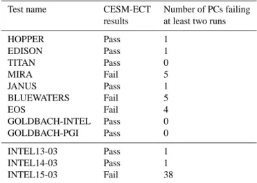
Now we present results for simulations in which we had less confidence in the expected outcome. These include running our default CESM simulation on other CESM-supported ma-chines as well as changing to a higher level of optimization on Yellowstone (−O3). We expected that the tests on other machines supported by CESM would pass, and, for each ma-chine, we list the machine name and location below (and give the processor and compiler type in parentheses). The effect of−O3 compiler options was not known as the CESM code base is large and level-three optimizations can be quite ag-gressive. The following simulations were performed.
– HOPPER: National Energy Research Scientific Com-puting Center (Cray XE6, PGI).
Table 1. CESM modifications expected to change the climate.
Test name CESM-ECT Number of PCs failing
results at least two runs
DUST Fail 9
FACTB Fail 36
FACTIC Fail 43
RH-MIN-LOW Fail 44
RH-MIN-HIGH Fail 30
CLDFRC-DP Fail 27
UW-SH Fail 24
CONV-LND Fail 33
CONV-OCN Fail 45
NU-P Fail 35
NU Pass 1
Table 2. CESM modifications expected to produce the same
cli-mate.
Test name CESM-ECT Number of PCs failing results at least two runs
NO-OPT Pass 1
INTEL-15 Pass 1
NO-THRD Pass 0
PGI Pass 0
GNU Pass 2
– EDISON: National Energy Research Scientific Com-puting Center (Cray XC30, Intel).
– TITAN: Oakridge National Laboratory (AMD Opteron CPUs, PGI).
– MIRA: Argonne National Laboratory (IBM BG/Q sys-tem, IBM).
– JANUS: University of Colorado (Intel Westmere CPUs, Intel).
– BLUEWATERS: University of Illinois (Cray XE6, PGI).
– EOS: Oakridge National Laboratory (Cray XC30, In-tel).
– GOLDBACH-INTEL: NCAR (Intel Xeon CPU cluster, Intel).
– GOLDBACH-PGI: NCAR (Intel Xeon CPU cluster, PGI).
– INTEL13-O3 Yellowstone with default Intel compiler and−O3 option.
– INTEL15-O3 Yellowstone with Intel 15.0.0 compiler and−O3 option.
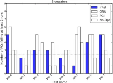
Note that we use the CESM-specified default compiler option for each CESM-supported machine. Table 3 indicates that most of the CESM-supported machine configurations pass (the nine test scenarios above the horizontal line), and the few that fail are all near the pass/fail threshold. In other words, these machine failures are in contrast to the more egregious failures obtained by changing CAM parameters as in Table 1. However, ideally all CESM-supported machines would pass our test (assuming the absence of error in their hardware and software environments), so a better understanding of the variability introduced by the environments of other machines (i.e., not Yellowstone) is needed. Therefore, as a first step, we ran additional tests on Mira and Bluewaters with the goal of better understanding (and substantiating) the failures in Ta-ble 3. For each machine, we ran seven more sets of three randomly perturbed simulations. Thus, we have a total of eight experiments each for Mira and Bluewaters, counting the original in Table 3. Furthermore, we created three addi-tional ensembles of 151 simulations based on the PGI, GNU, and NO-OPT scenarios listed in Sect. 4.2 and created a sum-mary file for each. Thus, we can test the eight new cases for consistency on both machines against a total of four ensem-bles to better understand the effect of the compiler on the consistency assessment. Results from these experiments are shown for Bluewaters and Mira in Figs. 3 and 4, respectively. Note that the Intel ensemble is the default “accepted” ensem-ble that we have used thus far in our experiments and the No-Opt option is also the Intel compiler (with−O0).
The results in Figs. 3 and 4 indicate that the compiler choice for the control ensemble on Yellowstone results in dif-ferences in the numbers of PC scores that fail each individual test case. However, the overall outcome from all four control ensembles is similar in that the test results are split in terms of passes and fails, indicating that these are in fact borderline cases for CESM-ECT with the current failure criteria, which requires at least three PCs to fail at least two runs. Test sce-narios that very nearly pass or fail, such as these for Blue-waters and Mira underscore the difficulty in distinguishing a bug in the hardware or software from the natural variabil-ity present in the climate system. Certainly we do not expect to perfect CESM-ECT to the point where a pass or fail is a definitive indication of the absence or presence of a prob-lem, though we have obtained a large amount of data to date that we will explore in detail to better characterize the effects of compiler and architecture differences on the variability. We expect to report on our further analysis in future work. Finally, another difficulty for our tool is that while PCA will indicate the existence of different signatures of variability be-tween new simulations and the ensemble, the differences de-tected may not necessarily be important in terms of the pro-duced climate and the decision on whether to accept or reject
BW-0 BW-1 BW-2 BW-3 BW-4 BW-5 BW-6 BW-7 Test name
0 1 2 3 4 5 6 7 8 9
Number of PCs failing at least 2 runs
Bluewaters
Intel GNU PGI No-Opt
Figure 3. Additional CESM-ECT results on Bluewaters, comparing
against four different ensemble distributions. Bars extending above the dashed line indicate an overall failure.
Mira-0 Mira-1 Mira-2 Mira-3 Mira-4 Mira-5 Mira-6 Mira-7 Test name
0 1 2 3 4 5 6 7 8 9
Number of PCs failing at least 2 runs
Mira
Intel GNU PGI No-Opt
Figure 4. Additional CESM-ECT results on Mira, comparing
against four different ensemble distributions. Bars extending above the dashed line indicate an overall failure.
that climate (e.g., because the definition of climate requires more than 1 year and involves spatial distributions).
Table 3. CESM modifications with unknown outcomes.
Test name CESM-ECT Number of PCs failing
results at least two runs
HOPPER Pass 1
EDISON Pass 1
TITAN Pass 0
MIRA Fail 5
JANUS Pass 1
BLUEWATERS Fail 5
EOS Fail 4
GOLDBACH-INTEL Pass 0
GOLDBACH-PGI Pass 0
INTEL13-03 Pass 1
INTEL14-03 Pass 1
INTEL15-03 Fail 38
5 CESM-ECT in practice
CESM-ECT has already been successfully integrated into the CESM software engineering workflow. In particular, the cre-ation of a new beta release tag in the CESM development trunk (that is not BFB with the previous tag) requires that CESM-ECT be run for the new tag on all CESM-supported platforms (e.g., the machines listed in Sect. 4.4 and the sup-ported compilers on those platforms (e.g, Intel, GNU and PGI, all with−O2, on Yellowstone). Results from these tests are kept in the CESM testing database. Failure on one or more of the test platforms signals that an error may exist in the new tag or on a particular machine, spawning an investi-gation and delay of the beta tag release.
CESM-ECT has proven its utility on numerous occasions, and we now provide several specific examples of the success of this consistency-testing methodology in practice. The first example concerns an early success for our ensemble-based testing methodology. The consistency test for a CESM.1.2 series beta tag test on the Mira machine failed decisively, while the consistency tests on all other platforms passed. The CESM-ECT failure prompted an extensive investigation of the Mira simulation data which resulted in the discovery that the CAM energy balance was incorrect. Eventually an error was discovered in the stochastic cloud generator code that only manifested itself on big-endian systems (Mira was the only big-endian machine in the group of CESM-supported machines). Because this particular success occurred early in the research and development stages of CESM-ECT (when we were initially looking at root-mean-squared Z scores), it provided the impetus to move forward and further refine our ensemble-based consistency-testing strategy.
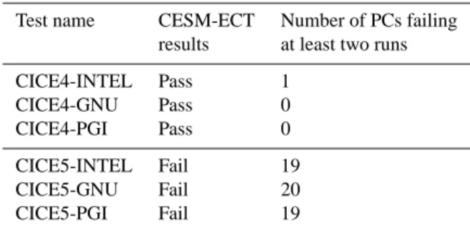
A second, more recent success for CESM-ECT was the detection of errors in a new version of the Community Ice Code (CICE). In particular, CICE5 replaced CICE4 in the CESM.1.3 series development trunk, and this upgrade was purported to not change the climate. However, when the
soft-ware tag with CICE5 was tested with CESM-ECT, failures occurred on all of the CESM-supported platforms. Recall that CESM-ECT uses an F compset (e.g., Sect. 4.1), which means that CICE runs in prescribed mode. Prescribed mode is intended for atmospheric experiments and uses the ther-modynamics in the sea ice model (the dynamics are deacti-vated) with a pre-specified ice distribution. The CESM-ECT failures for the new development tag raised a red flag that resulted in the detection and correction of a number of er-rors and necessary tuning parameter changes in the CICE5 prescribed mode. Pre-integration component-level testing for stand-alone CICE, however, allowed errors to go undetected in prescribed mode until run with CESM-ECT. Table 4 lists the results of CESM-ECT for three test scenarios on Yel-lowstone (Intel, GNU, and PGI compilers) with CICE5 and CICE4, showing that the difference was quite significant.
Finally, CESM-ECT has been essential in the evaluation of lossy compression schemes for CESM climate data. Lossy compression schemes result in data loss when the com-pressed data are reconstructed (i.e., uncomcom-pressed). Evalu-ating the impact of the loss in precision and/or accuracy in the reconstructed data is critical to the adoption of lossy com-pression methods in the climate modeling community. In par-ticular, we advocate for compression levels that result in re-constructed data that is not statistically distinguishable from the original data. The CESM ensemble-consistency method-ology has been invaluable in making this determination (e.g., Baker et al., 2014).
6 Conclusions and future work
Table 4. CESM development tag with two versions of the CICE
component run with different compilers on Yellowstone.
Test name CESM-ECT Number of PCs failing results at least two runs
CICE4-INTEL Pass 1
CICE4-GNU Pass 0
CICE4-PGI Pass 0
CICE5-INTEL Fail 19
CICE5-GNU Fail 20
CICE5-PGI Fail 19
– port-verification (new CESM-supported machines); – quality assurance for software release tags;
– exploration of new algorithms, solvers, compiler op-tions;
– feedback for model developers;
– detection of errors in the software or hardware environ-ment; and
– assessment of the effects of lossy data compression. Despite our successes with this new consistency-testing methodology, the natural variability present in the climate system makes the detection of subtle errors in CESM chal-lenging. While no verification tool can be absolutely correct, we consider CESM-ECT in its current form to be prelimi-nary work, as many avenues remain to be explored. We are currently conducting a more detailed analysis of large ensem-bles from different compilers and machines in an attempt to better characterize the effects of those types of perturbations. We have also begun to evaluate spatial patterns in addition to global (spatial) means, as these patterns may be revealing in such contexts as boundaries between ocean and land, and less chaotic systems like the coarse-resolution ocean. In addition, we are interested in other important climate statistics like ex-tremes. Finally, we intend to evaluate relationships between variables in cross-covariance studies.
Code availability
The software tools needed to test for ensemble consis-tency are included in the CESM public releases begin-ning with the version 1.4 series, which are available at https://github.com/CESM-Development/cime. Note that the Python testing tools can also be downloaded indepen-dently of CESM from the collection of parallel Python tools available on NCAR’s Application Scalability and Performance website (https://www2.cisl.ucar.edu/tdd/asap/ application-scalability) or obtained directly from NCAR’s public Subversion repository (https://proxy.subversion.ucar. edu/pubasap/pyCECT/tags/1.0.0/). CESM simulation data is available from the corresponding author upon request.
Appendix A: CAM variable list
The 134 total monthly variables output by default for CESM 1.3.x series include the 132 monthly variables listed at for CESM 1.2.2 at http://www.cesm.ucar.edu/models/cesm1.2/ cam/docs/ug5_3/hist_flds_fv_cam5.html, with the exception of the three variables ORO, dst_a1SF, and dst_a3SF. In addi-tion, five new variables are output:
– DTWR_H2O2 (wet removal Neu scheme tendency, 30 levels, in mol mol−1s−1)
– DTWR_H2SO4 (wet removal Neu scheme tendency, 30 levels, in mol mol−1s−1)
– DTWR_SO2 (wet removal Neu scheme tendency, 30 levels, in mol mol−1s−1)
– TAUGWX (zonal gravity wave surface stress, 1 level, in N m−2) and
– TAUGWY (meridional gravity wave surface stress, 1 level, in N m−2).
Note that for all experiments in this manuscript, the fol-lowing 14 variables were excluded for reasons of redun-dancy or zero variance: DTWR_H2O2, DTWR_H2SO4, DTWR_SO2, EMISCLD, H2SO4_SRF, ICEFRAC, LAND-FRAC, OCNLAND-FRAC, PHIS, SOLIN, TSMIN, TSMAX, SNOWHICE, AEROD_v. Because CESM-ECT allows the user to specify variables that should be excluded from the analysis, there is flexibility around the numbers of variables.
Acknowledgements. This research used computing resources provided by the Climate Simulation Laboratory at NCAR’s Computational and Information Systems Laboratory (CISL), sponsored by the National Science Foundation and other agencies. This research also used resources of the Oak Ridge Leadership Computing Facility at the Oak Ridge National Laboratory, which is supported by the Office of Science of the US Department of Energy under contract no. DE-AC05-00OR22725. This research used resources of the Argonne Leadership Computing Facility, which is a DOE Office of Science User Facility supported under contract no. DE-AC02-06CH11357. This research used resources of the National Energy Research Scientific Computing Center, a DOE Office of Science User Facility supported by the Office of Science of the US Department of Energy under contract no. DE-AC02-05CH11231. This work utilized the Janus supercomputer, which is supported by the National Science Foundation (award no. CNS-0821794) and the University of Colorado Boulder. The Janus supercomputer is a joint effort of the University of Colorado Boulder, the University of Colorado Denver and the National Center for Atmospheric Research.
References
Baker, A. H., Xu, H., Dennis, J. M., Levy, M. N., Nychka, D., Mickelson, S. A., Edwards, J., Vertenstein, M., and Wegener, A.: A methodology for evaluating the impact of data compression on climate simulation data, in: Proceedings of the 23rd interna-tional symposium on High-Performance Parallel and Distributed Computing, HPDC ’14, 203–214, 2014.
Carson II, J. S.: Model verification and validation, in: Proceedings of the 2002 Winter Simulation Conference, 52–58, 2002. Clune, T. and Rood, R.: Software testing and verification
in climate model development, IEEE Softw., 28, 49–55, doi:10.1109/MS.2011.117, 2011.
Dai, A., Meehl, G., Washington, W., Wigley, T., and Arblaster, J. M.: Ensemble simulation of 21st century climate changes: business as usual vs. CO2stabilization, B. Am. Meteor. Soc.,
82, 2377–2388, 2001.
Easterbrook, S. M. and Johns, T. C.: Engineering the software for understanding climate change, Comput. Sci. Eng., 11, 65–74, doi:10.1109/MCSE.2009.193, 2009.
Easterbrook, S. M., Edwards, P. N., Balaji, V., and Budich, R.: Guest editors’ introduction: climate change – science and soft-ware, IEEE Softw., 28, 32–35, 2011.
Goosse, H., Barriat, P., Lefebvre, W., Loutre, M., and Zunz, V.: In-troduction to climate dynamics and climate modeling, available at: http://www.climate.be/textbook (last access: 5 May 2015), 2014.
Hurrell, J. W., Holland, M. M., Gent, P. R., Ghan, S., Kay, J. E., Kushner, P. J., Lamarque, J. F., Large, W. G., Lawrence, D., Lindsay, K., Lipscomb, W. H., Long, M. C., Mahowald, N., Marsh, D. R., Neale, R. B., Rasch, P., Vavrus, S., Vertenstein, M., Bader, D., Collins, W. D., Hack, J. J., Kiehl, J., and Mar-shall, S.: The Community Earth System Model: a framework for collaborative research, B. Am. Metereol. Soc., 94, 1339–1360, doi:10.1175/BAMS-D-12-00121.1, 2013.
IPCC Data Collection Centre 2015, available at: http://www. ipcc-data.org/ (last access: 5 May 2015), 2015.
Kay, J., Deser, C., Phillips, A., A. Mai, A., Hannay, C., Strand, G., Arblaster, J., Bates, S., Danabasoglu, G., Edwards, J., Holland, M., Kushner, P., Lamarque, J.-F., Lawrence, D., Lindsay, K., Middleton, A., Munoz, E., Neale, R., Oleson, K., Polvani, L., and Vertenstein, M.: The Community Earth System Model (CESM) Large Ensemble Project: A Community Resource for Studying Climate Change in the Presence of Internal Climate Variabil-ity, B. Am. Meteorol. Soc., doi:10.1175/BAMS-D-13-00255.1, in press, 2015.
Oberkamf, W. and Roy, C.: Verification and Validation in Scien-tific Computing, Cambridge University Press, Cambridge, 13– 51, 2010.
Orsekes, N., K. Shrader-Frechette, K. Belitz: Verification, valida-tion, and confirmation of numerical models in the earth sciences, Science, 263, 641–646, 1994.
Orsekes, N.: Evaluation (not validation) of quantitative models, En-viron. Health Perspect., 106, 1453–1460, 1998.
Pipitone, J. and Easterbrook, S.: Assessing climate model software quality: a defect density analysis of three models, Geosci. Model Dev., 5, 1009–1022, doi:10.5194/gmd-5-1009-2012, 2012. Rosinski, J. M. and Williamson, D. L.: The
accumula-tion of rounding errors and port validaaccumula-tion for global at-mospheric models, SIAM J. Sci. Comput., 18, 552–564, doi:10.1137/S1064827594275534, 1997.
Sansom, P. G., Stephenson, D. B., Ferro, C. A. T., Zappa, G., and Shaffrey, L.: Simple uncertainty frameworks for selecting weighting schemes and interpreting multimodel ensemble cli-mate change experiments, J. Clicli-mate, 26, 4017–4037, 2013. Sargent, R. G.: Verification and Validation of Simulation Models,
in: Proceedings of the 2011 Winter Simulation Conference, 183– 198, 2011.
Shlens, J.: A Tutorial on Principal Component Analysis, CoRR, abs/1404.1100, available at: http://arxiv.org/abs/1404.1100 (last access: 5 May 2015), 2014.
von Storch, H. and Zwiers, F.: Testing ensembles of climate change scenarios for “statistical significance”, Clim. Change, 117, 1–9, 2013.
Whitner, R. B. and Balci, O.: Guidelines for selecting and using simulation model verification techniques, in: Winter Simulation Conference, 559–568, 1989.
Zhu, Y.: Ensemble forecast: a new approach to uncertainty and pre-dictability, Adv. Atmos. Sci., 22, 781–788, 2005.