ISSN 1546-9239
© Science Publications, 2004
A Causal Relationship between Inflation and
Productivity: An Empirical Approach for Romania
Nikolaos Dritsakis
Department of Applied Informatics
University of Macedonia, Economics and Social Sciences, Thessaloniki, Greece
Abstract: This study attempts to analyze the relationship between the productivity and the inflation of a transition country of the European Union as Romania. For this purpose we use quarterly data since 1990: IV in 2003: I and the causality analysis, which is based on an error correction model. The results of the empirical analysis showed that there is a causal relationship between inflation and productivity in the Romanian economy.
Key words: Productivity, Inflation, Granger Causality, Cointegration, Romanian Economy
INTRODUCTION
The starting point for the transition process in Romania was more difficult than in other countries in Central and Eastern Europe. Pre-transition policies emphasized self dependence, putting excessive focus on heavy industry and large infrastructure projects. This strategy led to the depletion of domestic energy sources and induced costly dependence on imports of energy and raw materials. During 1980s there was no growth in exports in order to repay the debt imports from the West. The technological lag increased significantly as a result. Towards the end of the 1980s the Romanian economy was on the verge of collapse and, unlike other transition economies, no attempts to reform had yet been tried.
Given this difficult legacy, the dominant political forces in place since the early 1990s advocated a gradualist approach, seeking to minimize the social costs associated with the transformation to market. The 1993 OECD Assessment of the Romanian economy pointed out clearly the risks associated with the delaying structural reforms. A key point in the Assessment was that, without deep restructuring of the economy, macroeconomic stabilization could not be sustained. Therefore, since 1993 the boost in exports and the apparent success in reducing inflation under the stabilization policy of Romanian economy were noted.
The Seville European Council (1996) encouraged Romania to pursue its efforts for accession in the European Union and also reiterated its commitment to provide full support of this candidate country.
Romania is expected to join the European Union on the basis of the same economic and political criteria that had been set by the Copenhagen and Madrid European Councils (1993, 1995) as well. As confirmed by the Laeken European Council (2002) the accession process is now irreversible.
The European Commission recommended, on the basis of the Copenhagen criteria, that Romania shouldn’t be included in the first group of countries with whom negotiations should be opened. Finally, Romania was invited at the Helsinki summit meeting in December 1999 to start negotiations for membership. The substantive negotiations started in March 2000.
Romania on the basis of the last Regular Report of European Union fulfills the political criteria as defined by the Copenhagen European Council (1993).
However, Romania still needs to improve legislative and decision making processes, while judiciary reforms should be made political priority. The government’s policy supports the institutions of human rights and protection of local minorities. Important steps were taken to implement the National Strategy for improving the Condition of Roma. Romania has continued to make progress towards being a functioning economy with the competitive market. Sustained and full implementation of planned measures together with the completion of the reform agenda should allow Romania to be able to cope with competitive pressure and market forces within the Union in the medium term.
The historic decision adopted by the EU at Helsinki meeting in December 1999 to include Romania in the group of candidate countries, signifies that Romania has moved to a new stage of its European integration process.
Economic integration is to be facilitated by bringing new opportunities for trade and as the economic environment becomes more attractive, by increasing foreign direct investment inflows. To this end, ‘‘Europe Agreement’’ provides the chance to Romania to have easier access in the economies of the European Union’s member states.
solid way to EU accession. Firstly, macroeconomic stability, without which there cannot be sustainable growth, is essential and secondly, inflation reduction in the level of 2% on the basis of the ‘‘Europe Agreement’’.
Trade liberalization and export growth in agricultural and industrial products consist the main target for economic restructuring. The abolition of tariff barriers allows the foreign direct investment growth in the domestic market.
Romania has concluded free-trade agreements with the European Union, EFTA, CEFTA, Moldova and Turkey. The basic principles of the agreement between Romania and European Union are:
• Trade liberalization
• Elimination of quantitative restrictions on imports
• Elimination of quantitative restrictions on exports
Romania’s commercial relations with the EU became predominant beginning in 1995. The share of exports to EU countries in the total Romanian exports increased from 33.9% in 1990-65.5% in 1999. The same trend was registered for Romanian imports from EU countries, whose share in total Romanian imports was 55.1% in 1999 compared with 21.8% in 1990. Among the candidate countries in 1999 (including Turkey, Cyprus and Malta), Romania was both the sixth largest destination for exports and the sixth largest source of imports in Europe.
The status of Romania as an EU candidate country should enhance its attractiveness to foreign investors. The Gross Domestic Product was 7.3% in 1997 and next year declined to 6.6%. The Copenhagen European Council (2002) set 2007 as the final date of accession to EU for Romania as full members.
While output continued to grow in 1996 fiscal policy was derailed under the impact of a largely unstructured economy. The official budget deficit was increased by quasi-fiscal items, such as the National Bank of Romania (NBR) refinancing of credits to the agricultural sector. This slippage resulted from pre-election policies in support of output and demand and a pervasive lack of financial discipline in large state-owned companies. With the rapid growth of the monetary base, inflation accelerated readily in such a point that World Bank halted their financial support.
Theoretical and Empirical Approaches: Inflation is
always a monetary phenomenon and productivity is a purely real occurrence. But upon reflection, we may reasonably think that inflation or at least things associated with it must matter for the firms' ability to
improve their productivity. In considering a link between inflation and productivity there are two possible causes directions: productivity affects inflation or inflation affects productivity. The first generally has higher productivity allowing cost reductions that flow through to product prices and thereby reduce inflation.
Higher productivity growth thus represents a positive supply shock that lowers inflationary pressures. The second effect posits that inflation affects productivity growth. From first principles, prices matter because they are a highly efficient means of transmitting the myriad of individual demand and supply decisions that occur throughout the economy[1]. In an inflationary environment, the price mechanism loses its efficiency. It seems plausible then, that when prices are changing frequently, firms may find it more difficult to distinguish an increase in the relative scarcity of their inputs from an across the board increase in prices. Similarly, the reduced certainty brought about by inflation increases the risk of entrepreneurial errors and would potentially induce lower levels of investment. This would all lower the overall productivity of the firm.
Early research into the inflation-productivity nexus was stimulated by the experience of high inflation of the 1970s and the subsequent fall in productivity growth. Most of the literature has debated the statistical question of whether the data support any relationship and if so, the causal direction. Minimal work explores the theoretical side, or how inflation may be transmitted into slower productivity growth and vice versa. The view was a little circumspect about the nature of any relationship between productivity growth and inflation. Nonetheless, both Keynesian and neoclassical theories suggest a negative relationship[2]. It is recognized that inflation has adverse effects on macroeconomic variables such as output and productivity growth[3,4].
[5]
Use a monetary model of endogenous growth and based on a panel of OECD and APAC countries using annual data for the period 1961-1997, they found that there is a negative effect of inflation and productivity for these countries.
direction from monetary to inflation and from inflation to growth for both accession countries[10].
Proposed two rationales for this occurrence: that the tax system’s lack of neutrality during periods of inflation increases the private sector’s tax burden and that inflation’s increasing variance with higher levels of inflation would cause sub-optimal resource allocations and increase the probability of entrepreneurial error, hence reducing investment. Using 1963-1979 Canadian data, Jarrett and Selody found a bi-directional relationship, with the rise in inflation explaining nearly the entire slowdown in productivity growth.
Another group of studies took up the debate in the mid 1990s. These had the advantage of being able to observe the productivity growth inflation relationship after the 1980s’ disinflation and also draw on the experience of a wider range of G7 economies[12,13].
Using annual data for the period 1951-1991 for Germany and 1955-1990 for USA respectively, suggested that there is not any causal relationship between productivity and inflation in both examined countries[14]. Resulted in the same conclusion in their research in Australia and New Zealand and also,[15] in their research for USA, United Kingdom, Canada, West Germany.
A further group of study is skeptical of any inflation productivity growth relationship. These studies take two tacks. One approach is to argue that the results show that the business cycle drives simultaneous variations in both productivity growth and inflation, not a long run relationship[16-18]. The stylized facts have productivity growth peaking ahead of the business cycle, with inflation then accelerating. In response, the monetary authorities increase interest rates, thus slowing output growth hence productivity growth through the effects of labor hoarding. Inflation’s slowdown lags that of the real economy. Thus, an appropriate model of the productivity growth inflation relationship must absorb the business cycle through variables such as real interest rates, the output gap, or variations in GDP growth.
The other critique argues the statistical point that productivity growth and inflation have different orders of integration[15,16,19,20]. These studies claim inflation is non-stationary while productivity growth is stationary and therefore there cannot be a long run relationship. Almost all the studies run Granger causality tests, or a close relative, VAR models. There does appear to be a relationship between productivity growth and inflation and where it is determinable, the causality appears to flow from inflation to productivity growth.
This study tries to investigate the direction of causality between inflation and productivity in Romania. It seems
That country has the most problems from all the other countries in transition and that’s the reason why we chose it. In the empirical analysis we used quarterly data for the period 1990: IV in 2003: I for the variables used.
Data and Methodological Issues: In order to test the causal relationship between the price level and the productivity of Romania, we use the following VAR model:
U = (CPI, PROD) (1) where: CPI is the price level PROD is the productivity
The data which are used in this investigation are quarterly, covering the period from 1990:IV to 2003:I and are derived from the databases of OECD (Main Economic Indicators), International Monetary Fund (IMF) and Datastream regarding 1995 as a base year.
All data are expressed by logarithms in order to include the proliferative effect of time series and are symbolized by the letter L preceding each variable name while ∆ denotes the first differences of these variables.
If these variables share a common stochastic trend and their first or second differences are stationary, then they can be cointegrated. Economic theory scarcely provides some guidance for which variables appear to have a stochastic trend and when these trends are common among the examined variables as well.
Initially, a bivariate VAR model of prices and productivity is estimated. Then, a four variable VAR model is introduced in order to account for potential influences of cyclical factors and changes in monetary policy on the price level-productivity relationship, two variables the real gross domestic product and the interest rate were added.
In order to test the existence of the statistical relationship among the examined variables, we pursue the following steps.
The first step is to verify the order of integration of the varied, since the causality tests are valid if the variables have the same order of integration. For the integration of these variables we used ADF test[21,22] and PP test[23].
approach[25-27]. The Engle-Granger method is based on the residual co integration test. The error correction model is employed to test directly for co integration between the two variables by examining the significance of the lagged level of the dependent variable.
Two additional variables are introduced in order to account for changes in real output and monetary policy. In this multivariate framework the co integration test is applied by using Johansen and Juselious approach,
which is based on the error correction representation of the VAR (p) model in conjunction with the Gaussian error model. This method tests for all numbers of co integrated vectors between the variables. It uses all variables as endogenous ones, thus avoiding an arbitrary choice of the dependent variable. Finally, it provides a unified framework for the estimation and the co integrated relations test within the framework of the vector error correction model.
Evidence of co integration rules out the possibility of the estimated relationship being spurious. As long as the four variables have a common trend, causality in the Granger sense and not in the structural sense, should exist in at least one direction. Although co integration implies the presence of Granger causality, it does not necessarily identifies the direction of causality between variables. This Granger causality can be captured through the vector error correction model derived from the long-run co integrated vectors[28,29].
Thus, the third step involves utilization of the vector error correction model for testing the causality among the model variables[24]. Claim that in the presence of co integration, there always exists a corresponding error correction representation, which implies that changes in
the dependent variable are a function of the level of imbalance in the co integrated relationship captured by the Error Correction Term (ECT). Thus, through the error correction term (ECM), model VECM establishes an additional way to examine the Granger causality.
The non-significance of ECT is referred to as a long-run non-causality. The absence of short-long-run causality is established by the non-significance of the sum of the largess of each explanatory variable. Finally, the non-significance of all the explanatory variables including the ECT term in the VECM indicates the absence of Granger causality.
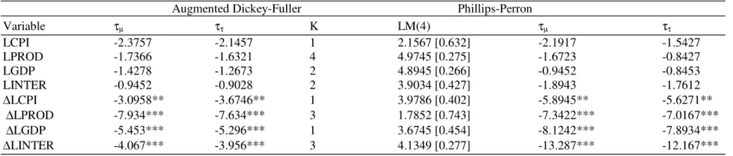
Data stationary tests: To examine the stationarity of
the mentioned variables of the model (1), we have used the[21,22] tests, but also[23] test. The results of these tests appear in Table 1. The minimum values of the[30] and[31] statistics indicated that the ‘best’ ADF equations were those including an intercept and trend and the corresponding numbers of lagged terms. As far as the autocorrelation disturbance term test is concerned, the Lagrange Multiplier LM (4) test has been used.
The results of Table 1 suggest that the null hypothesis of a unit root in the time series cannot be rejected in variable levels at a 1, 5 and 10% levels of significance. Therefore, no time series appear to be stationary in varying levels. When the time series are transformed into first differences they become stationary and consequently the related variables can be characterized integrated of order one, i.e. They are I (1). Moreover, for all variables the LM (4) test first differences show that there is no serial correlation in the disturbance terms.
Table 1: Tests of Unit Roots Hypothesis
Augmented Dickey-Fuller Phillips-Perron
Variable τµ ττ K LM(4) τµ ττ
LCPI -2.3757 -2.1457 1 2.1567 [0.632] -2.1917 -1.5427
LPROD -1.7366 -1.6321 4 4.9745 [0.275] -1.6723 -0.8427
LGDP -1.4278 -1.2673 2 4.8945 [0.266] -0.9452 -0.8453
LINTER -0.9452 -0.9028 2 3.9034 [0.427] -1.8943 -1.7612
∆LCPI -3.0958** -3.6746** 1 3.9786 [0.402] -5.8945** -5.6271**
∆LPROD -7.934*** -7.634*** 3 1.7852 [0.743] -7.3422*** -7.0167***
∆LGDP -5.453*** -5.296*** 1 3.6745 [0.454] -8.1242*** -7.8934***
∆LINTER -4.067*** -3.956*** 3 4.1349 [0.277] -13.287*** -12.167***
Notes: The relevant tests are derived from the OLS estimation of the following auto-regression for the variable involved:
t 0 1 t 1 2 t i t
i 1 i
X X t X u
κ
− −
=
∆ = δ + δ + δ +
∑
Φ ∆ + (2)Table 2: Bivariate Co integration Tests
Dependent
Variable Productivity Dependent variable price level
Method k t-test k t-test
Engle-Granger 3 -3.4245 3 -4.9861
Error Correction 2 -4.0561 2 -3.9674
Estimates
Notes: The augmented D-F test is based on the equation (2) with constant and without trend, where ut is the estimated residual from the
long-run model LCPIt = α0 + α1LPRODt + ut (3) The lag length k is
chosen so the estimated residuals of the equation (2) will be without autocorrelation. The critical values for the rejection of the null hypothesis of no co itegration between the two variables at 1, 5 and 10% are –3.90, -3.33 and –3.04, respectively.
Table 3: Johansen and Juselious Co integration Tests Variables LCPI, LPROD, LGDP, LINTER (VAR = 4)
Maximum Eigenvalues
--- Critical values ---
Null Alternative Eigenvalue 95% 90%
r = 0 r =1 38.43 31.00 28.32
r < 1 r = 2 15.38 24.35 22.26
Trace Statistic
r = 0 r >1 60.73 58.93 55.01
r < 1 r = 2 22.32 39.33 36.28
Table 4: Equation specification tests
Equation ---
Tests LCPI LPROD LGDP LINTER
Serial Correlation 1.23 0.82 0.44 0.19
ARCH (4) 0.78 0.26 1.27 0.34
Normality 7.56 1.08 2.15 10.67
Heteroskedasticity 2.14 1.45 0.96 0.72
Notes: Test for normality follow X2 distribution, all the others follow F-distribution
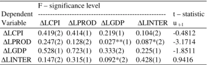
Table 5: Causality Test Results Based on Vector Error – Correction Modeling
F – significance level
Dependent --- t – statistic Variable ∆LCPI ∆LPROD ∆LGDP ∆LINTER u t-1
∆LCPI 0.419(2) 0.414(1) 0.219(1) 0.104(2) -0.4812
∆LPROD 0.247(2) 0.128(2) 0.027**(1) 0.087*(2) -3.1714
∆LGDP 0.528(1) 0.723(1) 0.333(2) 0.225(1) -1.8511
∆LINTER 0.147(2) 0.315(1) 0.092*(2) 0.428(1) 0.9416 Notes: *, ** and *** indicate 10, 5 and 1% levels of significance Number in parentheses are lag lengths.
Co integration Test: In this section, by applying the[23] method and estimating the error correction model, it has been examined if there is any co integration relationship between the productivity and the price level in the examined country since these two variables are integrated of order one.
The results of co integration analysis using the Engle- Granger method and an error-correction model are presented in Table 2 testing for the significance of the coefficient of the lagged level of the dependent variable. The results suggest that the hypothesis of no co integration for the two variables, namely the price level and the productivity, is rejected.
Then in order to investigate the effects on the real production and also on the monetary policy, two more variables are added to the VAR model, namely the gross domestic product and the interest rate. The results of co integration analysis of the four variables using the Johansen maximum likelihood approach is presented in Table 3. This approach tests for the number of co integrated vectors among the examined variables. Further, this approach uses all the variables as endogenous ones, thus avoiding the arbitrary choice of the dependent variable. Finally, it provides a unified framework for the estimation and the test of co integrated relationships within the framework of the vector error correction model.
Given the fact that in order to apply the Johansen approach a sufficient number of time lags is required, we have followed the relative procedure, which is based on the calculation LR (Likelihood Ratio) test statistic[32]. The results showed that the value ρ=2 is the appropriate specification for the relationship. In addition, each equation of the VAR system passes a series of diagnostic tests including serial correlation, ARCH (4), normality and heteroskedasticity tests.
Table 4 reports the specification tests for the VAR (4) system. The tests do not reveal any misspecification accept the rejection of normality for price level and interest rate. From the results we can infer that there is a long-run relationship between the price level, the productivity, the real production, the interest rate for Romania for the examined period. Therefore, the relationships can be used as an error correction mechanism in the VAR model.
VAR model with an error correction mechanism:
After determining that the logarithms of the model variables are co integrated, we must then estimate a VAR model in which we shall include a Mechanism of Error Correction model (MEC). The error correction model derived from the long run co integration relationship, has the following form:
∆LCPIt = lagged(∆LCPIt, ∆LPRODt, ∆LGDPt,
∆LINTERt ) + λut-1 + Vt (5)
where, ∆ is reported to all variables’ first differences ut-1 are the estimated residuals from the co integrated regression (long-run relationship) and represent the deviation from the equilibrium in the time period t.
Table 6: Summary of Causal Relations
CPI →PROD CPI →GDP CPI →INTER PROD →CPI PROD →GDP PROD →INTER
2 2 2
GDP →CPI GDP →PROD GDP →INTER INTER →CPI INTER →PROD INTER →GDP
1,2 1 1,2 2
Vt is a 4X1 vector of white noise errors[29]. Suggested that there are two channels of causality, the first one is obtained through the lagged variables (∆LPROD, ∆LGDP, ∆LINTERt), when the coefficients of all these variables are statistically significant (F distribution) and the second channel is raised in case the (λ) coefficient of the variable ut-1 is statistically significant (t-distribution). If λ is statistically significant in the equation (5) productivity, real gross domestic product and interest rate effect on the price level.
The error correction model (Equation 5) is used to investigate the causal relationships among the model variables.
The single equation error correction model is estimated for LCPI and LPROD:
k k
t 0 1 t 1 2 t 1 t i t i t
i 1 i i 1 i
Y X− X− Y− X− u
= =
∆ = α + α + α + β ∆
∑
+∑
γ ∆ + (4)The reported values are t tests for the estimated coefficient α1. The critical values for α1 at 1, 5 and 10% for N = 50 are -4.32, -3.67 and -3.28, respectively.
This analysis provides the short run dynamic adaptation to the long run equilibrium. The levels of significance of F-distribution test for the Granger causality, while with t-distribution the ut-1 coefficient is examined as well. The numbers in parentheses are the lag lengths determined by using the Akaike criterion. As discussed earlier, there are two channels of[29], which are called channel 1 and channel 2. If the coefficients of the lagged values of the variables (apart from the coefficients of the lagged values of the dependent variable) on the right hand side in equation 5 are jointly significant, then this is called channel 1. On the other hand, if the coefficient of the lagged value of the error correction term is statistically significant, then this is called channel 2. For convenience, discussing the results, let us call the relationships a “strong causal relation” if it is through both channel 1 and channel 2and simply a “causal relation” if it is through either channel 1 or channel 2.
From the results of Table 6 we can infer that there is a unidirectional Granger causality between the price level and the productivity with direction from the price level to the productivity. This result is in accordance with the study of [6, 9, 7,8] as well. The price level and the
productivity cause the gross domestic product for the examined period, while there is a bi-directional causal relationship between the gross domestic product and the interest rate. Finally, we can see that there is a dynamic causal relationship between the real gross domestic product and the productivity and also between the interest rate and the productivity.
CONCLUSION
The purpose of this study was to examine the subject of Granger causality between the price level and the productivity in a transition country to European Union such as Romania using quarterly data for the period 1990: IV-2003:I through the multivariate causality analysis, which is based on an error correction model. For this reason, the latest time series methods have been used such as unit root tests, the bivariate and the multivariate co integration tests and vector error correction models.
Especially, the Augmented Dickey-Fuller (ADF) and Phillips-Perron (PP) tests have been used for the existence of unit root test. On this basis, the bivariate co integration analysis has been used, as suggested by Engle-Granger and the estimation of the error correction model, while the Johansen and Juselious estimation method has been applied for the multivariate co integration.
Although Romania has high relative inflation rates for the studied period, the results of empirical analyses suggested that there is a long run relationship between the producer and the price level in both techniques of co integration analysis which have been used, as well as in the multivariate co integration analysis adding two more variables, which consist changes in real production such as gross domestic product and also in monetary policy such as the interest rate.
Then an error correction model’s methodology has been used to estimate the short run and long run relationships. The selected vectors gave us the error correction terms, which proved to be statistically significant in 5 and 10% levels of significance respectively of the variables of the productivity and the real gross domestic product.
and productivity cause the gross domestic product, while there is a bilateral causal relationship between gross domestic product and interest rate. Finally, there is a dynamic causal relationship between the gross domestic product and the productivity, but also between the interest rate and the productivity for the examined period.
REFERENCES
1. Bulman, T. And J. Simon, 2003. Productivity and Inflation, Research Discussion Paper, No 2003-10 Bank of Australia.
2. Lucas, R., 1973. Some international evidence on output-inflation tradeoffs. Am. Econ. Rev., 63: 326-334.
3. Bitros, G. And E. Panas, 2001. Is there an inflation-productivity trade-off? Some evidence from the manufacturing sector in Greece. Applied Econ., 33: 1961-969.
4. Dritsakis, N., 2003. Hungarian macroeconomic variables – reflection on causal relationships. Acta Oeconomica, 53: 61-73.
5. Gillman, M., M. Harris and L. Matyas, 2004. Inflation and growth: Explaining a negative effect. Empirical Economics, 29: 149-167.
6. Clark K.P., 1982. Inflation and the productivity decline. American Economic Rev., 72: 149-154. 7. Buck, A. And F. Fitzroy, 1988. Inflation and
productivity growth in the federal republic of Germany. J. Post Keynesian Econ., 10: 428-444. 8. Saunders, P. And B. Biswas, 1990. An empirical
Note on the relationship between Inflation and Productivity in the United Kingdom, British Review of Economic Issues, 12: 67 – 77.
9. Ram, R., 1984. Causal Ordering Across Inflation and Productivity Growth in the Post-War United States, The Review of Economics and Statistics, 66: 472 – 477.
10. Jarrett J.P. And J. G. Selody, 1982. The Productivity-Inflation Nexus in Canada, The Review of Economics and Statistics, 64: 361-67. 11. Gillman, M. And A. Nakov, 2003. Granger
Causality of the Inflation-Growth Mirror in Accession Countries, Economics of Transition (forthcoming).
12. Smyth D.J., 1995a. Inflation and Total Factor Productivity in Germany, Weltwirtschaftliches Archiv, 131: 403 - 405.
13. Smyth D.J., 1995b. The Supply Side Effects of Inflation in the United States: Evidence from Multifactor Productivity, Applied Economic Letters, 2: 482 – 483.
14. Chowdhury, A. And G. Mallik, 1998. A Land Locked into low Inflation: How Far is the Promised Land?, Economic Analysis and Policy, 28: 233 – 243.
15. Cameron, N., D. Hum and W. Simpson, 1996. Stylized Facts and Stylized Illusions: Inflation and Productivity Revisited, Canadian J. Economics, 29: 152 - 162.
16. Sbordone, A. And K. Kuttner, 1994. Does Inflation Reduce Productivity? Federal Reserve Bank of Chicago, Economic Perspectives, 18: 2 - 14. 17. Freeman D .G. And D. Yerger, 1997. Inflation and
Total Productivity in Germany: A Response to Smyth, Weltwirtschaftliches Archiv, 133: 158 - 163.
18. Freeman D .G. And D. Yerger, 2000. Does Inflation Lower Productivity? Time Series Evidence on the Impact of Inflation on Labor Productivity in 12 OECD Nations, Atlantic Economic J. 28: 315 – 332.
19. Tsionas, E., 2001. Euro-Land: and Good for the European South? J. Policy Modeling, 23: 67– 81. 1. 19.Tsionas, E., 2003. Inflation and Productivity:
Empirical Evidence from Europe, Review of International Economics, 11:114 – 129.
20. Dickey, D.A. and W.A. Fuller, 1979. Distributions of the Estimators for Autoregressive Time Series with a Unit Root. J. Am. Stat. Assoc., 74: 427 – 431.
21. Dickey, D.A. And W.A. Fuller, 1981. Likelihood Ratio Statistics for Autoregressive Time Series with a Unit Root. Econometrica, 49: 1057–1072. 22. Phillips, P. C. B. And P. Perron, 1988. Testing for
a Unit Root in Time Series Regression. Biometrics, 75: 335 – 346.
23. Engle, R.F. And C.W.J. Granger, 1987. Co integration and Error Correction: e-presentation, Estimation and Testing. Econometrica, 55: 251 - 276.
24. Johansen, S., 1988. Statistical Analysis of Co integration Vectors, J. Economic Dynamics and Control, 12: 231 – 254.
25. Johansen, S. And K. Juselius, 1990. Maximum Likelihood Estimation and Inference on Co integration with Applications to the Demand for Money, Oxford Bulletin of Economics and Statistics, 52: 169 - 210.
27. Granger, C.W.J., 1986. Developments in the Study of Co integrated Economic Variables. Oxford Bulletin of Economics and Statistics, 48: 213 - 228.
28. Granger, C.W.J., 1988. Developments in a Concept of Causality, J. Econometrics, 39, 199 – 211. 29. Akaike, H., 1973. Information Theory and an
Extension of the Maximum Likelihood Principle, In: Petrov, B. And Csaki, F. (Eds) 2nd International Symposium on Information Theory. Budapest: Akademiai Kiado.
30. Schwartz, R., 1978. Estimating the Dimension of a Model. Annals of Statistics, 6: 461 – 464.