PREDIZENDO DEFEITOS DE SOFTWARE COM
CÉSAR FRANCISCO DE MOURA COUTO
PREDIZENDO DEFEITOS DE SOFTWARE COM
TESTES DE CAUSALIDADE
Tese apresentada ao Programa de Pós--Graduação em Ciência da Computação do Instituto de Ciências Exatas da Universi-dade Federal de Minas Gerais como req-uisito parcial para a obtenção do grau de Doutor em Ciência da Computação.
Orientador: Roberto da Silva Bigonha
Coorientador: Marco Túlio de Oliveira Valente,
Nicolas Anquetil
Belo Horizonte
CÉSAR FRANCISCO DE MOURA COUTO
PREDICTING SOFTWARE DEFECTS WITH
CAUSALITY TESTS
Thesis presented to the Graduate Program in Ciência da Computação of the Univer-sidade Federal de Minas Gerais in partial fulfillment of the requirements for the de-gree of Doctor in Ciência da Computação.
Advisor: Roberto da Silva Bigonha
Co-Advisor: Marco Túlio de Oliveira Valente,
Nicolas Anquetil
Belo Horizonte
c
2013, César Francisco de Moura Couto. Todos os direitos reservados.
Couto, César Francisco de Moura
C871p Predicting Software Defects with Causality Tests / César Francisco de Moura Couto. — Belo Horizonte, 2013
xxiii, 106 f. : il. ; 29cm
Tese (doutorado) — Universidade Federal de Minas Gerais
Orientador: Roberto da Silva Bigonha
1. Defect Prediction; Causality; Software Metrics; Granger Test. I. Título.
This thesis is dedicated to my wife Cinthia, who has always supported me.
Acknowledgments
This work would not have been possible without the support of many people.
I thank God to provide me the discipline and persistence to reach a Ph.D. degree.
I thank my wife Cinthia, who has had patience in difficult moments and has always been at my side.
I thank my whole family—especially my father Célio, my mother Cecília, my brothers Mila, Carol, and Celinho, and my mother-in-law Dalva—for having always supported me.
I thank my advisors M. T. Valente and R. S. Bigonha for the lessons, attention, availability, and patience.
I thank my co-advisor N. Anquetil for giving me the opportunity to work under his supervision in France.
I thank the members of the ASERG research group—especially R. Terra and C. Maffort—for the friendship and technical collaboration.
I thank the professor N. Vieira for the lessons during my teaching activities.
I thank the Department of Computer Science at UFMG, for the opportunity to participate its PhD program.
I would like to express my gratitude to the member of my thesis defense committee—E. Figueiredo (UFMG), R. Assunção (UFMG), D. Serey (UFCG), and P. C. Masiero (USP).
Resumo
Predição de defeitos é uma área de pesquisa em engenharia de software que objetiva identificar os componentes de um sistema de software que são mais prováveis de ap-resentar defeitos. Apesar do grande investimento em pesquisa objetivando identificar uma maneira efetiva para predizer defeitos em sistemas de software, ainda não existe uma solução amplamente utilizada para este problema. As atuais abordagens para predição de defeitos apresentam pelo menos dois problemas principais. Primeiro, a maioria das abordagens não considera a idéia de causalidade entre métricas de soft-ware e defeitos. Mais especificamente, os estudos realizados para avaliar as técnicas de predição de defeitos não investigam em profundidade se as relações descobertas indicam relações de causa e efeito ou se são coincidências estatísticas. O segundo problema diz respeito a saída dos atuais modelos de predição de defeitos. Tipicamente, a maioria dos modelos indica o número ou a existência de defeitos em um componente no fu-turo. Claramente, a disponibilidade desta informação é importante para promover a qualidade de software. Entretanto, predizer defeitos logo que eles são introduzidos no código é mais útil para mantenedores que simplesmente sinalizar futuras ocorrências de defeitos.
Para resolver estas questões, nós propomos uma abordagem para predição de defeitos centrada em evidências mais robustas no sentido de causalidade entre métricas de código fonte (como preditor) e a ocorrência de defeitos. Mais especificamente, nós usamos um teste de hipótese estatístico proposto por Clive Granger (Teste de Causalidade de Granger) para avaliar se variações passadas nos valores de métricas de código fonte podem ser usados para predizer mudanças em séries temporais de defeitos. Nossa abordagem ativa alarmes quando mudanças realizadas no código fonte de um sistema alvo são prováveis de produzir defeitos. Nós avaliamos nossa abordagem em várias fases da vida de quatro sistemas implementados em Java. Nós alcançamos um precisão média maior do que 50% em três dos quatro sistemas avaliados. Além disso, ao comparar nossa abordagem com abordagens que não são baseadas em testes de causalidade, nossa abordagem alcançou uma precisão melhor.
Abstract
Defect prediction is a central area of research in software engineering that aims to identify the components of a software system that are more likely to present defects. Despite the large investment in research aiming to identify an effective way to pre-dict defects in software systems, there is still no widely used solution to this problem. Current defect prediction approaches present at least two main problems in the cur-rent defect prediction approaches. First, most approaches do not consider the idea of causality between software metrics and defects. More specifically, the studies per-formed to evaluate defect prediction techniques do not investigate in-depth whether the discovered relationships indicate cause-effect relations or whether they are statistical coincidences. The second problem concerns the output of the current defect prediction models. Typically, most indicate the number or the existence of defects in a component in the future. Clearly, the availability of this information is important to foster soft-ware quality. However, predicting defects as soon as they are introduced in the code is more useful to maintainers than simply signaling the future occurrences of defects.
To tackle these questions, in this thesis we propose a defect prediction approach centered on more robust evidences towards causality between source code metrics (as predictors) and the occurrence of defects. More specifically, we rely on a statistical hypothesis test proposed by Clive Granger to evaluate whether past variations in source code metrics values can be used to forecast changes in time series of defects. The Granger Causality Test was originally proposed to evaluate causality between time series of economic data. Our approach triggers alarms whenever changes made to the source code of a target system are likely to present defects. We evaluated our approach in several life stages of four Java-based systems. We reached an average precision greater than 50% in three out of the four systems we evaluated. Moreover, by comparing our approach with baselines that are not based on causality tests, it achieved a better precision.
List of Figures
1.1 Overview of defect prediction approaches . . . 3
1.2 Variables and techniques used by defect prediction approaches . . . 4
1.3 Proposed approach to predict defects . . . 6
2.1 Buggy code detected by FindBugs in the Apache Lucene . . . 15
2.2 FindBugs warning example . . . 15
2.3 Example of class with a warning generated by PMD . . . 15
2.4 PMD warning example (for the class showed in Figure 2.3) . . . 16
3.1 Time series of metric values and defects in a hypothetical system . . . 31
3.2 Simulated time series yt=yt−1+ǫt and y0 = 2 . . . 33
3.3 NOM for Eclipse JDT core . . . 34
3.4 NOPM and NOM’ time series. The increase in NOPM values just before bi-week 21 has been propagated to NOM’ few weeks later . . . 36
3.5 Examples of Granger Causality between LOC and defects. . . 37
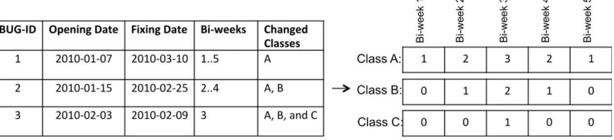
3.6 Bayesian network representing dependencies among five variables [Pea00] . 38 4.1 Example of extracting the time series of defects . . . 45
4.2 Time series for a Eclipse JDT class . . . 47
4.3 Defects time series (for a Eclipse JDT class) . . . 48
4.4 Time series for the systems in our dataset . . . 49
5.1 Series LOC and number of defects for a class of the Eclipse JDT system . 52 6.1 Steps to build a model for defect prediction . . . 62
6.2 Example of a threshold for the LOC metric . . . 63
6.3 Defect prediction model . . . 64
6.4 Hypothetical example of calculation precision and recall . . . 68
6.5 Training and validation time series (Eclipse JDT Core) . . . 68
6.6 True alarms (TA), precision (Pre), recall (Rec), and F-measure (F) . . . . 69
6.7 True alarms raised by our approach . . . 71
6.8 Precision results . . . 73
6.9 Precision results ofBaseline1 and Baseline2 . . . 74
6.10 Recall results . . . 75
6.11 Number of alarms and true alarms, for different threshold functions (Eclipse JDT Core) . . . 77
6.12 Distribution of bugs by severity . . . 78
7.1 BugMaps architecture . . . 83
7.2 History Browser . . . 85
7.3 Snapshot Browser . . . 85
7.4 BugMaps-Granger’s architecture . . . 86
7.5 Granger browser . . . 88
7.6 Bug as Entity browser . . . 89
7.7 Granger results per class . . . 90
7.8 Bug as entity . . . 91
7.9 The top-10 defective classes . . . 92
7.10 Number of time series with a positive result for Granger-causality . . . 93
List of Tables
2.1 Other object-oriented metrics . . . 13
2.2 Empirical studies on CK metrics and defect prediction . . . 18
2.3 Empirical studies on process metrics and defect prediction . . . 20
2.4 Empirical studies on warnings and defect prediction . . . 21
2.5 Classification of the maintenance requests . . . 22
2.6 Precision and recall . . . 24
4.1 Original dataset . . . 41
4.2 Extended dataset . . . 42
4.3 Metrics considered in our dataset . . . 43
4.4 Number of bugs, defects, and defects per bugs . . . 46
4.5 Size properties . . . 46
5.1 RSS and Adjusted R2 for the bivariate and univariate autoregressive models 52 5.2 Percentage and absolute number of classes conforming to preconditions P1, P2, and P3 . . . 56
5.3 Percentage of time series conforming successively to preconditions P4 and P5 57 5.4 Percentage and absolute values of classes with n positive results for Granger 57 5.5 Classes, Granger positive classes (GPC), number of bugs, number of defects, number of defects in Granger positive classes (DGC) . . . 58
5.6 Granger positive p-values . . . 59
5.7 Percentage of lags with a positive result for Granger-causality (highest val-ues in bold) . . . 59
6.1 Confusion matrix . . . 67
6.2 Average precision (Pre) and recall (Rec) results considering alternative threshold functions . . . 76
7.1 Source code metrics considered by BugMaps-Granger . . . 87
Contents
Acknowledgments xi
Resumo xiii
Abstract xv
List of Figures xvii
List of Tables xix
1 Introduction 1
1.1 Motivation . . . 1
1.2 Research Challenges on Defect Prediction . . . 3
1.3 Thesis Statement . . . 5
1.4 Thesis Outline . . . 8
2 Background 9 2.1 Software Quality and Defect Prediction . . . 9
2.2 Software Metrics . . . 10
2.2.1 Source Code Metrics . . . 11
2.2.2 Process Metrics . . . 13
2.2.3 Warnings from Bug Finding Tools . . . 14
2.3 Defect Prediction Approaches . . . 16
2.3.1 Source Code Metrics Approaches . . . 17
2.3.2 Process Metrics Approaches . . . 18
2.3.3 Bug Finding Tools Approaches . . . 20
2.3.4 Application of Causality Tests in Software Maintenance . . . 25
2.3.5 Critical Appraisal on Defect Prediction Approaches . . . 25
2.4 Final Remarks . . . 27
3 Prediction Techniques 29 3.1 Linear and Logistic Regression . . . 29 3.2 Critical Appraisal on Regression . . . 30 3.3 Granger Causality . . . 32 3.3.1 Stationary Time Series . . . 32 3.3.2 Granger Test . . . 34 3.4 Other Causality Techniques . . . 37 3.5 Final Remarks . . . 39
4 Dataset 41
4.1 Original Dataset . . . 41 4.2 Extended Dataset . . . 42 4.2.1 Time Series of Source Code Metrics . . . 43 4.2.2 Time Series of Defects . . . 44 4.3 Provided Time Series . . . 46 4.4 Related Datasets . . . 48 4.5 Final Remarks . . . 49
5 Feasibility Study 51
5.1 Granger Test Application . . . 51 5.2 Applying the Granger Test . . . 53 5.3 Setup and Results . . . 54 5.3.1 Preconditions on Time Series of Defects . . . 55 5.3.2 Preconditions on Time Series of Source Code Metrics . . . 56 5.3.3 Defects Covered by Granger . . . 56 5.3.4 Lags Considered by Granger . . . 58 5.4 Final Remarks . . . 60
6 Predicting Defects Using Granger 61
6.1 Proposed Approach . . . 61 6.2 Thresholds to Trigger Alarms . . . 62 6.3 Defect Prediction Model . . . 63 6.4 Evaluation . . . 64 6.4.1 Evaluation Setup . . . 65 6.4.2 Results . . . 69 6.5 Threats to Validity . . . 77 6.6 Final Remarks . . . 79
7 BugMaps-Granger 81 7.1 Motivation . . . 81 7.2 BugMaps . . . 83 7.3 BugMaps-Granger . . . 85 7.3.1 Architecture . . . 86 7.4 Case Study . . . 89 7.5 Related Tools . . . 92 7.6 Final Remarks . . . 93
8 Conclusion 95
8.1 Summary . . . 95 8.2 Contributions . . . 96 8.3 Further Work . . . 97
Bibliography 99
Chapter 1
Introduction
In this chapter, we start by presenting our motivation (Section 1.1) and current research challenges on defect prediction (Section 1.2). Next, we present our thesis statement and an overview of our approach for predicting defects in software systems (Section 1.3). Finally, we present the outline of this thesis (Section 1.4).
1.1
Motivation
The primary goal of software engineering is to produce high quality software [Mey00, p. 3]. However, producing software that is fast, reliable, easy to use, readable, and well-structured is not a simple task. Software development is a complex and challeng-ing task because it involves a number of technologies, practices, and methodologies, such as requirements specification, programming languages, databases, design patterns, platforms, frameworks, and processes.
On the other hand, software maintenance is as complex and challenging as soft-ware development. It involves tasks such as: (a) corrective maintenance that concerns fixing bugs; (b) adaptive maintenance that corresponds to adaptations in software to changes in its environment; (c) perfective maintenance that deals with improving or adding new features in the system’s requirements; and (d) preventive maintenance that concerns activities aiming to increase the system’s maintainability [LS80]. Soft-ware maintenance takes up most part of softSoft-ware cost [LS80, NP90, Mey00, Som09]. According to Sommerville, 50%–75% of the total software costs concern the mainte-nance tasks [Som09, Ch. 9]. In this total cost, 17% concerns corrective maintemainte-nance tasks, 18% corresponds to adaptive maintenance tasks, and 65% deals with perfective and preventive maintenance tasks.
2 Chapter 1. Introduction
The high cost of maintenance is influenced by various factors. Among these fac-tors, we can mention the complexity of the problem domain, the turnover of developers, the lack of documentation, and the low quality of the source code under maintenance. Particularly, some studies investigated the impact of the low quality of the source code on the maintenance costs [LB85, Cor89, Vis10]. Lehman and Belady were among the first to observe that as a software system increases in size and complexity, its quality decreases and its maintenance becomes harder [LB85]. Corbi showed that 50%–60% of the time of a maintenance task is spent understanding the source code [Cor89]. Ac-cording to Visser, low quality software systems are resistant to change, because the more complex, unstructured, or tangled is the source code, the higher is the time spent to perform a maintenance task [Vis10].
On the other hand, evaluating a software system in order to improve its overall quality is also a challenging task. Meyer has proposed a set of properties that can be used to evaluate software quality [Mey00, p. 3]. According to Meyer, software quality can be evaluated by external factors, i.e., those factors perceived by users, and internal factors, i.e., those factors only perceived by the development team (developers and maintainers). Among the external quality factors, we can mention properties such as efficiency, correctness, robustness, extensibility, reusability, and ease of use. On the other hand, the internal quality factors include properties such as coupling, cohesion, readability, modularity, separation of concerns, etc.
In recent decades, many metrics have been proposed to evaluate both internal and external software properties [Hum95, FP97, Kan02, LMD05, Pre10]. For example, in-ternal quality factors can be measured by source code metrics, including properties such as coupling, cohesion, size, inheritance, complexity, and violations in recommended programming practices. On the other hand, the external quality can be measured for example by the number of bugs reported by the users and developers.1
In summary, these metrics provide a quantitative indication of some properties of a software system. Therefore, designers, developers, and maintainers can rely on these metrics to evaluate and control the internal and external quality of a software system. Potentially, such quality control can prevent future problems, as the occurrence of bugs.
Particularly, the number of bugs is an important measure to evaluate the relia-bility (correctness and robustness as proposed by Meyer [Mey00]) of software systems. Reliability is a critical external factor because it can impair the success of the product ahead stakeholders and increase the costs of corrective maintenance tasks. Therefore, knowing in advance the chances that a system has to fail in the future is essential to
1
1.2. Research Challenges on Defect Prediction 3
increase its reliability, and ultimately its quality. In this context, defect prediction is an important area of research in software engineering that aims to identify the components of a system that are more likely to fail [BBM96, SK03, NB05a, NBZ06, MPS08, Has09]. Clearly, the availability of this information is of central value to most software quality assurance procedures. For example, it allows quality managers to allocate more time and resources to test, redesign, and reimplement those components predicted as defect-prone [ZNZ08]. In general, the aforementioned quality assurance procedures can reduce the amount of corrective maintenance and therefore improve customer’s satisfaction.
Figure 1.1 summarizes the typical scheme followed by the state-of-the-art in de-fect prediction approaches [HBB+12]. Typically, these approaches work by retrieving information on a system such as bug history (extracted from bug tracking platforms) and source code versions (extracted from version control platforms), computing soft-ware metrics, and after that building prediction models to identify the components of a software that are defect-prone. More specifically, current defect prediction ap-proaches aim to determine the number of defects (during a period of analysis) in a software component. Basically, the defects of a component are compared to other properties (measured by software metrics) to infer which properties typically correlate with defects. The ultimate goal is to construct a model that predicts the number or the existence of defects in a component in a future time frame.
Source Code
Bugs
Defect Prediction
Model
Component
Defects
Software Metrics
Figure 1.1: Overview of defect prediction approaches
1.2
Research Challenges on Defect Prediction
4 Chapter 1. Introduction
of the independent variable, and the validation technique [HBB+12]. Figure 1.2 sum-marizes the variables and techniques involved in current defect prediction approaches. The independent variables include source code metrics, change metrics, warnings is-sued by bug finding tools, and violations in recommended programming practices (or code smells). The modeling techniques include linear regression, logistic regression, naïve bayes, neural networks, decision tree. The granularity of the prediction can be at the file/class/method level or module/package level. The validation phase can rely on classification and ranking techniques.
Classification Ranking Defect Prediction Approaches Validation Techniques Modeling Techniques Independent Variables Linear Regression Logistic Regression Naîve Bayes Neural Network Decision Tree Granularity of Independent Variables File Class Method Package Module
Source Code Metrics Bug Finding Tools Code Smells Change Metrics Complexity Coupling Cohesion Inheritance Size Code churn Bug fixes Entropy of changes
Figure 1.2: Variables and techniques used by defect prediction approaches
1.3. Thesis Statement 5
well known that regression models cannot filter out spurious correlations [Ful94]. The second problem we identified concerns the output of the current defect predic-tion models. As described in Secpredic-tion 1.1, typically the output of such predicpredic-tion models indicate the number or the existence of defects in a component in the future. Clearly, the availability of this information is important to foster software quality. However, predicting defects as soon as they are introduced in the source code, e.g., identifying the changes to a class that are more likely to generate defects, is more useful to the maintainer than simply signaling the future occurrences of defects (since defects are expected anyway in most real-world software components).
1.3
Thesis Statement
Our thesis statement is as follows:
Reliable and precise defect prediction techniques play a pivotal role on soft-ware quality assessment and improvement. However, the state-of-the-art defect prediction approaches are centered on techniques that have not been designed to capture temporal cause-effect relations. Therefore, the main goal of this work is to propose a new defect prediction model centered on causal relations over time series of source code metrics and software defects. The proposed model triggers defect alarms whenever changes made to the source code of a target system have a high chance of producing defects.
6 Chapter 1. Introduction
specifically, we aim to identify the changes to a class that are more likely to generate defects. For this purpose, our approach relies on input from the Granger Test to trig-ger alarms as soon as changes that are likely to introduce defects in a class are made. Therefore, we claim that our model contributes directly to improve software quality.
Figure 1.3 details our approach for defect prediction. In a first step, we apply the Granger Causality Test to infer possible causalities between historical values of source code metrics and the number of defects in each class of the system under analysis. In this first step, we also calculate a threshold for variations in the values of source code metrics that in the past Granger-caused defects in such classes. For example, suppose that a Granger-causality is found between changes in the size of a given class in terms of lines of code (LOC) and the number of defects in this class. Considering previous changes in this specific class, we can establish for example that changes adding more than 50 lines of code are more likely to introduce defects (more details on how such thresholds are calculated are presented in Chapter 6). Using these thresholds and the Granger results calculated in the previous step, a defect predictor analyzes each change made to a class and triggers defect alarms when similar changes in the past Granger-caused defects.
Defect Prediction
Model Past changes like that Alarm!
Granger-caused defects
Granger Test
Granger results Alarm thresholds
Changed class Source code metrics
Defects Time Series
Figure 1.3: Proposed approach to predict defects
To develop the proposed thesis, we performed the following tasks:
1.3. Thesis Statement 7
Conference on Software Quality [ACSV10]. Later, this study was extended and published in the Software Quality Journal [CASV13]. The methodology, dataset, results, and lessons learned after this first study are described in Chapter 2.
2. We extended a dataset made public by D’Ambros et al. to evaluate defect predic-tion techniques [DLR10]. Basically, we extended this dataset: (a) by extracting again all source code versions considered in the dataset and recalculating the source code metrics; (b) by almost doubling the number of source code versions included in the original dataset, and (c) by introducing the time series of defects. This dataset is part of the COMETS dataset, which generated a communication in Software Engineering Notes [CMGV13]. Chapter 4 describes our extension to D’Ambros et al. dataset.
3. We conducted a second study to investigate the feasibility of applying Granger to detect causal relationships between time series of source code metrics and defects. Particularly, our goal was to evaluate whether there are causal relation-ships between source code metrics and defects in the classes of object-oriented systems. This study resulted in a working paper in the Brazilian Conference on Software Quality [CVB11] and full paper in the European Conference on Soft-ware Maintenance and Reengineering [CSV+
12]. The methodology, results, and lessons learned after this second study are described in Chapter 5.
4. We developed and evaluated an approach for predicting defects using causality tests. More specifically, we leveraged the experience and knowledge gained after the studies described in the previous items to propose and validate a model that triggers alarms whenever changes made to the source code of a target system have a high chance of producing defects. Chapter 6 describes the steps we followed to construct and evaluate this model.
8 Chapter 1. Introduction
1.4
Thesis Outline
This thesis is structured in the following chapters:
• Chapter 2 provides a general discussion on software quality and defect prediction and presents the software metrics commonly used to predict defects. This chapter also presents the state-of-the-art in defect prediction.
• Chapter 3 presents an overview on the Granger Causality Test and describes other techniques commonly used for predicting defects.
• Chapter 4 describes our dataset including time series of source code metrics and defects, extracted for four real world systems (Eclipse JDT Core, Eclipse PDE UI, Equinox, and Lucene).
• Chapter 5 describes a feasibility study designed to illustrate and to evaluate the application of Granger on defects prediction.
• Chapter 6 describes the defect prediction approach proposed in this work, as well its evaluation.
• Chapter 7 presents the BugMaps tool for the visual exploration and analysis of bugs, including the visualization of causal relations between source code metrics and bugs.
Chapter 2
Background
In this chapter, we start by providing a discussion about software quality and defect prediction (Section 2.1). Next, we present the software metrics commonly used by defect prediction approaches (Section 2.2). Finally, we present the state-of-the-art in defect prediction (Section 2.3) and provide a critical appraisal on current defect prediction approaches.
2.1
Software Quality and Defect Prediction
The primary goal of software engineering is to produce high quality software. Software quality is the degree to which a software meets its requirements specification [Sta90]. On the other hand, software quality assurance consists of a set of activities necessary to provide adequate confidence that a software conforms to its requirements specifi-cation [Sta90]. Among the software quality activities, we can mention code review, refactoring, testing, measuring the impact of changes, keeping records and reporting (bugs, improvements, and new features), configuration management, release manage-ment, product integration, etc.
To clarify how defect prediction approaches might be useful for ensuring software quality, suppose a scenario where a version of a given software will be released but the developer leader suspects that there are defects in some source code modules. To find these defects, the developer leader can rely on some resources responsible for ensuring software quality, such as code reviewers, senior developers, and testers. However, these resources are limited and represent a high cost to the software project. Therefore, the developer leader want to spend them in the most effective way, getting the best software quality and the lowest risk of defects. More specifically, he wants to spend
10 Chapter 2. Background
the most quality assurance resources on those modules that need it most, i.e., those modules that have high chances of producing defects.
On the other hand, allocating quality assurance resources is not a simple task. If a module without defects is tested or reviewed over a long period, this may indicate a non-optimal allocation of resources. If a module with defects is not tested or reviewed enough, a defect can appear in the field (i.e., defects reported by final users) causing more serious problems, such as corrective maintenance and stakeholders dissatisfaction. Therefore, identifying defect-prone modules may help the development leader to decide where the software quality assurance resources must be allocated before releasing a new version of a target software. Particularly, the quality assurance resources can perform tasks such as source code inspection, unit testing, functional testing, etc. Such tasks can improve the reliability of the software under development, reducing the number of future corrective maintenance tasks and improving the customer satisfaction.
In summary, knowing in advance the chances that a system has to fail in the future is a desirable way to obtain a more correct and robust software. It is in this context that the studies on defect prediction are addressed. Various defect prediction approaches have been proposed in recent decades [BBM96, SK03, NB05a, NBZ06, MPS08, Has09]. These approaches analyze historical information about a target software—such as bug history and source code evolution—in search of indicators about the presence of future defects. For example, a simple defect prediction approach can rely on the number of past defects as an indicator of future defects, i.e., software modules that had many defects in the past might have more chances of future defects. Among other metrics used as indicators of defects, we can mention source code metrics, code change metrics, warnings issued by bug finding tools, design flaws, etc.
In the following sections, some important software metrics used by defect predic-tion approaches are presented and the state-of-the-art in defect predicpredic-tion is reviewed. Finally, an evaluation of the current works on defect prediction is presented.
2.2
Software Metrics
2.2. Software Metrics 11
software metrics are usually classified into three categories: process metrics, project metrics, and product metrics [Kan02, Pre10], as described next:
• Process metrics: enable the organization to evaluate the process used to con-struct a software system. More specifically, a software process defines techniques, management methods, tools, people, and tasks related to the software develop-ment. Therefore, process metrics can be used to improve software development and maintenance practices. As examples, we can mention defects per KLOC or function point, change metrics, number files involved in bug fixing, etc.
• Project metrics: enable the organization to evaluate the progress of a software project. Basically, project metrics describe the project characteristics and exe-cution. Number of developers, cost, schedule, and productivity are examples of project metrics.
• Product metrics: enable the software engineers to evaluate the internal properties of a software product. As examples of product metrics, we can mention size, complexity, coupling, cohesion, and inheritance.
Particularly, in this thesis, we focus on process and product metrics, since they have been used as independent variables in several defect prediction approaches. Among the product metrics already used to construct defect prediction models, we can mention source code metrics (including complexity, coupling, cohesion and size metrics) [BBM96, BWD+
00, SK03, GFS05, DLR10] and warnings reported by bug finding tools [NB05a, ZWN+06, WAWS08, ASV11, CASV13]. On the other hand, process metrics such as code change metrics are used by other defect prediction mo-dels [GKMS00, NB05b, Has09, MPS08]. Finally, we are not aware of works that use project metrics to predict defects.
2.2.1
Source Code Metrics
Several defect prediction approaches reported in the literature are centered on source code metrics [BBM96, BWD+
00, SK03, GFS05, DLR10]. Typically, such approaches consider that the current design and structure of the software influence the presence of future defects. Basically, they do not analyze the version history of the system, but only its current codebase, by using a variety of source code metrics.
12 Chapter 2. Background
(WMC), Depth of Inheritance Tree (DIT), Number of Children (NOC), Coupling be-tween Object Class (CBO), Response for a Class (RFC), and Lack of Cohesion in Methods (LCOM) [CK91, CK94]. These metrics are described next:
• WMC: represents the complexity of the class as measured by its methods. The calculation of the metric is given by the sum of the complexity of the methods in the class. However, the definition of complexity remains open. According to Chidamber and Kemerer, WMC is an indicator of how much time and effort are required to develop and maintain a given class.
• DIT: indicates the depth of a class in the inheritance tree, which is given by the length of the path from the class to the root of the tree. DIT is nowadays considered an indicator of design complexity.
• NOC: denotes the number of immediate subclasses of a class. This metric is an indicator of the importance that a class has in the system. If a class has a large number of children, it might for example require more tests.
• CBO: indicates the number of classes to which a certain class is coupled to. For Chidamber and Kemerer, a coupling between two classes exists when methods implemented in one class use methods or instance variables defined by other classes. This metric can be used to reveal design problems. For example, it is widely accepted that excessive coupling is harmful to modular design, because the more independent a class is, more easy is to reuse it in other applications.
• RFC: indicates the number of methods that can be called in response to a message received by a class, defined as the number of methods of the class plus the number of methods invoked by them. RFC is considered an indicator of coupling.
• LCOM: indicates the lack of cohesion between the methods in a class. Chidamber and Kemerer consider that cohesion between methods is defined by the use of common instance variables. LCOM is the number of method pairs that have no instance variables in common minus the number of method pairs with common instance variables. Therefore, the smaller the value of LCOM, the more cohesive is the class.
2.2. Software Metrics 13
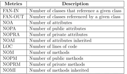
metrics, we can mention lines of code (LOC), number of public methods (NOPM), FAN-IN, FAN-OUT, etc.
Table 2.1: Other object-oriented metrics
Metrics Description
FAN-IN Number of classes that reference a given class FAN-OUT Number of classes referenced by a given class NOA Number of attributes
NOPA Number of public attributes NOPRA Number of private attributes NOAI Number of attributes inherited LOC Number of lines of code
NOM Number of methods NOPM Number of public methods NOPRM Number of private methods NOMI Number of methods inherited
Finally, D’ambros et al. proposed a metric called entropy of source code to predict defects [DLR10, DLR12]. The basic idea consists in measuring the evolution of source code metrics through the variations of a metric over subsequent sample versions. The more spread the variations of the metric, the higher is the entropy. For example, suppose that the WMC of a system is 100, but only one class contributes to this result. For this source code metric, the entropy is low. On the other hand, if the WMC of a system is 100, but 10 classes have contributed equally to achieve this result, this means that the entropy is high.
2.2.2
Process Metrics
Process metrics are also used by studies on defect prediction [GKMS00, NB05b, MPS08, Has09, DLR12, KSA+13]. Typically, defect prediction approaches based on process metrics consider that information extracted from version control systems—such as source code changes—can be used to predict defects. These approaches assume that code that changes a lot is more defect-prone than stable code. For example, Ball et al. introduced the concept of code churn as a measure of the “amount of code change taking place within a software unit over time” [NB05b]. As example of code churn, we can mention number of changed files and the sum of lines of code added, changed, and deleted between two versions.
14 Chapter 2. Background
file was involved in bug-fixing activities. To calculate this metric, the authors used pat-tern matching on the comments available in the commit operations. For determining whether a revision is a bug fix, the revision comment must match the string “%Fix%” and must not match the strings “%prefix%” and “%postfix%”. On the other hand, Zim-mermann et al relied on the convention that the IDs of the bugs are included in the comments of commits in bug fix operations [ZPZ07]. In other words, to be classified as a bug fix, the revision comments must include a reference to the bug ID. In this thesis, we adopted a similar strategy as described in Section 4.2.2.
Hassan introduced the metric entropy of changes, in order to measure the com-plexity of code changes [Has09]. Basically, this metric measures how distributed are the changes in the files of a target system during a time interval. The more spread is a change, the higher its complexity. The intuition is that a change that affects only a single file is simpler than one that affects several files. Therefore, this metric is an indicator of the complexity of code changes.
2.2.3
Warnings from Bug Finding Tools
Several bug finding tools have been proposed to detect software defects by means of static analysis techniques [NB05a, ZWN+
06, WAWS08, ASV11, CASV13]. Basically, defect prediction approaches based on bug finding tools try to infer relationships be-tween the warnings issued by such tools and defects. In this section, we provide an overview of the FindBugs and PMD tools, which are commonly used in defect predic-tion approaches [HP04, Cop05].
FindBugs is an open-source tool that relies on static analysis to look for more than four hundred bug patterns in Java bytecode [HP04]. Bug patterns are coding idioms that are likely to represent errors and are classified into categories such as thread/synchronization correctness, malicious code, performance, etc. Bug patterns are also assigned high, medium, or low priorities. FindBugs internal architecture includes components for intraprocedural control and data flow analysis. These components are responsible for making a sequential search through the bytecode to detect bug patterns. Figure 2.1 shows an example of a potential buggy code detected by FindBugs in the classQueryParser from the Apache Lucene system1
. The catch block (line 1071) is empty, i.e., the exception is being ignored. Figure 2.2 shows the warning message generated by FindBugs after analyzing this code fragment. This warning indicates that exceptions should be handled or thrown out by the target method.
1
2.2. Software Metrics 15
996: final public Query Term(String field) throws ParseException { ...
1069: try {
1070: fms = Float.valueOf(fuzzySlop.image.substring(1))... 1071: } catch (Exception ignored) { }
... 1237: }
Figure 2.1: Buggy code detected by FindBugs in the Apache Lucene
DE: Method might ignore exception (DE_MIGHT_IGNORE)
This method might ignore an exception. In general, exceptions should be handled or reported in some way, or they should be thrown out of the method.
Figure 2.2: FindBugs warning example
PMD is another open-source tool that uses static analysis to identify potential problems in Java source code and to check coding styles [Cop05]. For example, PMD rulesets are able to detect empty statements, dead code, duplicated code, inappropriate coupling, untrusted code, etc. Different from FindBugs, PMD requires the source code of the target program. Basically, PMD parses the source code in order to create an Abstract Syntax Tree (AST). To detect violations, PMD checks this AST against predefined rulesets.
Figure 2.3 shows an example of a code smell (i.e., a violation in recommended programming practices) detected by PMD in the classLuceneMethodsfrom the Apache
Lucene system. The method invertDocument has some nested if statements (lines
295 to 296). For this method, PMD generates the warning described in Figure 2.4, which recommends that the nested if should be combined in a single statement.
286: private void invertDocument(Document doc) { ...
295: if (field.isIndexed()) { 296: if (field.isTokenized()) { 297: Reader reader;
... 338: }
16 Chapter 2. Background
<violation
beginline="296" endline="329" begincolumn="9" endcolumn="9" rule="CollapsibleIfStatements" ruleset="Basic"
package="lucli" class="LuceneMethods" method="invertDocument"
externalInfoUrl="http://pmd.sourceforge.net/rules/..." priority="3">
These nested if statements could be combined
</violation>
Figure 2.4: PMD warning example (for the class showed in Figure 2.3)
2.3
Defect Prediction Approaches
A recent systematic literature review identified 208 defect prediction studies—including some of the works that will be presented in this section—published from January 2000 to December 2010 [HBB+12]. The studies differ in terms of the software metrics used for prediction, the modeling technique, the granularity of the independent variable, and the validation technique. Typically, the independent variables are associated to source code metrics, change metrics, previous defects, warnings issued by bug finding tools, design flaws, etc. The modeling techniques vary with respect to linear regression, logistic regression, naïve bayes, neural networks, etc. The granularity of the prediction can be at the method level, file/class level, or module/package level. The validation are usually conducted using classification or ranking techniques.
2.3. Defect Prediction Approaches 17
2.3.1
Source Code Metrics Approaches
The source code properties as measured by CK metrics received considerable attention for the purposes of defect prediction, as can be observed in Table 2.2. Basili et al. were among the first to investigate the use of CK metrics as early predictors for fault-prone classes [BBM96]. In a study on eight medium-sized systems they used logistic regression to analyze the relationship between metrics and fault-prone classes. This study revealed that there is a correlation between CK metrics (with the exception of the LCOM metric) and such classes.
Briand et al. discovered that several design metrics from the CK suite were pos-itively associated with fault-prone classes [BWIL99, BWD+00]. More specifically, the frequency of method invocations (related to CBO and RFC) and the depth of inheri-tance hierarchies (related to DIT) are associated with fault-prone at the level of classes. Cartwright and Shepperd studied the inheritance measures derived from the CK suite (DIT and NOC) in an industrial object-oriented system implemented in C++ [CS00]. They concluded that both measures have an influence on the defect density of classes. Emam et al. used the CK metrics and Briand’s coupling metrics [BDW99] to predict fault-prone classes in a commercial Java system [EMM01]. The results indicated that inheritance (DIT) is strongly associated with fault-prone classes.
Subramanyam and Krishnan investigated the relation between defects and CK metrics, such as CBO, WMC, and DIT [SK03]. In their study, they evaluated a single e-commerce system with modules implemented in C++ and Java. For modules in C++, they found that WMC, DIT, and CBO with DIT have a relevant impact on the number of defects. For the modules implemented in Java, only CBO with DIT has had an impact on defects. Gyimothy et al. performed an analysis similar to the study conducted by Basili et al. [BBM96] using CK metrics and lines of code (LOC) as predictors for fault-prone classes [GFS05]. They showed that CBO is among the best metrics for fault prediction and LOC is the second metric with the best results.
D’ambros et al. provided the original dataset with the historical values of the source code metrics that will be used in this thesis [DLR10]. By making this dataset publicly available, their goal was to establish a common benchmark for comparing bug prediction approaches. They relied on this dataset to evaluate a representative set of prediction approaches reported in the literature, including approaches based on CK metrics, the object-oriented metrics showed in Table 2.1, change metrics, bug fixes, and entropy of changes. The results indicated that CK metrics yielded a poor predictor with an unstable behavior among the analyzed systems.
18 Chapter 2. Background
Table 2.2: Empirical studies on CK metrics and defect prediction
Study Indep. Variable Model Technique Results
[BBM96] CK suite Logistic Regression WMC, DIT, RFC, CBO, and NOC
contributed to predict faults. LCOM did not contribute to predict faults. [BWIL99] CBO, RFC, and LCOM Logistic Regression CBO, RFC, and LCOM were
asso-ciated with fault-prone of classes. [BWD+
00] CK suite Logistic Regression WMC, CBO, DIT, RFC and NOC
were associated with fault-prone of classes. LCOM was not associated with faults.
[CS00] DIT and NOC Linear Regression DIT and NOC had influence on the de-fect density of classes.
[EMM01] DIT and NOC Logistic Regression DIT is associated with fault-prone. [SK03] WMC, CBO, and DIT Linear Regression WMC, CBO, and DIT had a relevant
impact on the number of defects.
[GFS05] CK suite Logistic Regression,
Linear Regression, and others
CBO contributed to predict faults.
[DLR10] CK suite Linear Regression CK suite yielded a poor predictor.
in their models [NBZ06, HPH+09]. However, such studies did not analyze the CK suite individually, but combined with other source code metrics. For example, Nagappan et al. conducted a study on five components of the Windows operating system in order to investigate the relationship between source code metrics and field defects [NBZ06]. They concluded that source code metrics indeed correlate with defects. However, they highlight that there is no single set of metrics that can predict defects in all the five Windows components. As a consequence of this finding, the authors suggest that software quality managers can never blindly trust on metrics, i.e., in order to use metrics as early bug predictors we must first validate them using the project’s history [ZNZ08]. Later, the study of Nagappan et al. was replicated by Holschuh et al. using a large ERP system (SAP R3) [HPH+09]. They confirmed the results obtained by Nagappan et al. in the this new system. However, both studies rely on linear regression models and correlation tests, which consider only an “immediate” relation between the independent and dependent variables. On the other hand, the dependency between bugs and source code metrics may not be immediate, i.e., usually there is a delay or lag in this dependency. In this thesis, we presented a new approach for predicting bugs that considers this lag.
2.3.2
Process Metrics Approaches
de-2.3. Defect Prediction Approaches 19
fects. Table 2.3 shows some of the approaches in the literature that rely on process metrics to predict defect-prone modules. As we can observe, Graves et al. reported a study based on the fault history of the modules of a large telephone switching sys-tem [GKMS00]. They found that lines of code and other standard source code metrics are generally poor predictors of faults. On the other hand, they argued that process metrics—such as number of modifications, the age of a file, size of the modifications, etc.—are better predictors of future faults.
Nagappan and Ball analyzed the code churn between the releases of the Win-dows Server 2003 and WinWin-dows Server 2003-SP1 to predict the defect density in later release [NB05b]. They found that relative code churn (e.g., normalized by the number of lines of code) is able to predict system defect density with high levels of statisti-cal significance. Moser et al. used data extracted from the version control system of the Eclipse project, such as source code metrics (including complexity, size, etc.) and change metrics (including code churn, files committed together, number of times a file was involved in bug-fixing, etc.) to predict a code unit either as defect free or defec-tive [MPS08]. The results indicated that for the Eclipse data, process metrics can be used as predictors of defective code unit.
Hassan analyzed six open source projects to validate the hypothesis that the more complex the changes to a file, the higher the chances this file will contain faults [Has09]. He found two main results: (i) the number of prior faults is a better predictor for future faults than the number of prior modifications; (ii) the complexity of the code change is a better predictor for future faults than prior modifications or prior faults. D’ambros et al. also used process metrics as independent variable in their models [DLR12]. The authors proposed two new metrics called churn and entropy of source code metrics. Their results showed that churn and entropy of source code achieved the best adjusted R2 and Spearman coefficient in four out of the five analyzed systems.
Typically, defect prediction models are used to identify defect-prone files or pack-ages. Kamei et al. proposed a new approach for defect prediction called “Just-In-Time Quality Assurance” that focus on identifying defect-prone software changes instead of files or packages [KSA+
20 Chapter 2. Background
Table 2.3: Empirical studies on process metrics and defect prediction
Study Indep. Variable Model Technique Results
[GKMS00] Change Metrics Linear Regression Change metrics can be use as predictor of future faults.
[NB05b] Change Metrics Logistic Regression and Linear Regres-sion
Code churn is able to predict system defect density.
[MPS08] Change Metrics and Source Code Metrics
Logistic Regression and others
Change metrics can be used as defect predictors defective code unit. [Has09] Entropy of Changes Linear Regression The more complex the changes to a
file, the higher the chance the file will contain faults.
[DLR12] Churn and Entropy of Code Metrics
Linear Regression Entropy and churn had a better per-formance than CK metrics.
[KSA+
13] Change Metrics Linear Regression Change metrics can to cover 62% of the defects.
In this thesis, we trained our models using data from a time frame and validated them using data from future time frames.
2.3.3
Bug Finding Tools Approaches
Basically, these approaches use warnings reported by bug finding tools as early indica-tors of future defects, as summarized in Table 2.4. As we can observe, Nagappan and Ball described an experiment to measure the correlation between warnings reported by static analysis tools and defects [NB05a]. By using Spearman’s test, the authors found a positive correlation between the density of warnings issued by the PREfix/PREfast tools and the density of pre-release defects detected in the Windows Server 2003. In addition, they rely on linear regression to build models to predict the ability of PRE-fast/PREfix to predict future defects. The results showed that bug finding tools can be used as early indicators of defects.
Zheng et al. analyzed three systems developed at Nortel Networks using three commercial static analysis tools: Gimpel’s FlexeLint2
, Reasoning’s Illuma3
, and Klock-work’s inForce and GateKeeper4
[ZWN+06]. They followed the GQM process to de-termine the economical implications of using static analysis tools. The authors showed that the number of warnings raised by static analysis tools can be a fairly good indicator of fault prone modules.
Wagner et al. evaluated the effectiveness of bug finding tools in two large sys-tems [WAWS08]. In their work, they considered two tools: FindBugs and PMD. The
2.3. Defect Prediction Approaches 21
Table 2.4: Empirical studies on warnings and defect prediction
Study Indep. Variable Model Technique Validation Technique
[NB05a] PREfix/PREfast warnings Linear regression Spearman Correlation [ZWN+06] Automated static analysis
(ASA)
– Spearman Correlation and
Preci-sion Measures [WAWS08] FindBugs and PMD
war-nings
– Removed Warnings Rate and
Spearman Correlation [ASV11] FindBugs and PMD
war-nings
– Removed Warnings Rate
[CASV13] FindBugs warnings – Precision and Recall
goal was to assess the effectiveness of such tools to detect defects that occur in the field. For the first evaluated system, they did not find a single warning generated by FindBugs and PMD that could be related to a field defect. For the second system, they found a direct correspondence between four warnings and field defects. The authors concluded that bug finding tools are not effective to prevent field defects, since a small number of defects were detected.
Araujo et al. reported a study on the lifetime of the warnings reported by the FindBugs and PMD tools in five stable releases of the Eclipse platform [ASV11]. The authors classified a warning as relevant when it was removed some time after its first appearance in the system. They concluded that when the analysis is restricted to just warnings in the correctness category, 68.9% of the warnings were removed in later versions of the target system. Another conclusion was that PMD is not an effective tool to report relevant warnings, since only 26% of the warnings issued by this tool were classified as relevant.
2.3.3.1 Static Correspondence between FindBugs Warnings and Defects
We conducted our own study to investigate whether the warnings issued by bug finding tools are related to defects [ACSV10, CASV13]. More specifically, the study evaluates whether the warnings issued by FindBugs are useful to predict the program elements that must be changed in order to remove field defects (bugs reported in bug tracking platforms). In this study, we analyzed three medium size systems: Rhino (a JavaScript interpreter with 31 KLOC that is developed as part of the Mozilla project),
ajc (an AspectJ compiler, with around 63 KLOC), and Lucene (an information
22 Chapter 2. Background
Study Setup: We consider that there is a static correspondencebetween a warning w reported by FindBugs and a field defectd whenwis reported in the program elements that must be changed to fix d. For the first two systems, we relied on information available at the iBugs repository5
. iBugs stores the source code before and after the correction of several defects reported by the users of the systems. The iBugs repository provides information about 32 issues (an issue may be a field defect, an improvement, or a new feature) reported by the Rhino’s users. These issues were reported via Bugzilla6
, the bug tracking platform used by the Rhino’s development team. In addition, the iBugs repository has information about 348 issues reported for the ajc compiler. For
Lucene, we relied on the information available in the Jira bug tracking platform used by the Apache Foundation7
. We considered information about 90 issues for Lucene. We performed the following tasks to collect data to assess the static correspon-dence between warnings and field defects:
1. We filtered the issues that denote corrective maintenance tasks, since it makes no sense to expect a bug finding tool based on static analysis to predict the need of new features and improvements. For Rhino and ajc, we read and evaluated
the text of each issue reported via Bugzilla. Our goal was to distinguish between issues that represent field defects and issues that in fact are improvements or new features. For Lucene, the filtering process was simpler, because Jira provides a search facility that allows to select only issues that are field defects. Table 2.5 reports the number of issues classified as corrective maintenance and as the other maintenance types. As can be observed, the percentage of corrective requests has been 50% (for Rhino), 66% (for ajc), and 33% (for Lucene).
Table 2.5: Classification of the maintenance requests
Maintenance types Rhino ajc Lucene
Qty % Qty % Qty %
Corrective 16 50 231 66 30 33 Other types 16 50 117 34 60 67
Total 32 100 348 100 90 100
2. We downloaded the source code before and after each issue we classified as cor-rective. For Rhino and ajc, the source code was retrieved directly from the iBugs
repository. For Lucene, the source code was retrieved from the SVN version con-trol platform, using the ID of the SVN transaction responsible for fixing a given
5
http://www.st.cs.uni-saarland.de/ibugs
6
http://www.bugzilla.org
7
2.3. Defect Prediction Approaches 23
bug b(this ID is provided by the Jira issue tracking platform). Moreover, we also retrieved from SVN the version of the system with an identifier equal to (ID-1), i.e., the version just before fixing the bug b.
3. We automatically compared the versions before and after fixing the considered field defects in order to find the defective methods. In our context, a defective method is a method changed to fix a field defect. We relied on a small parser for Java in order to calculate the changed methods8
. By traversing the Abstract Syntax Tree (AST) generated by this parser, it was possible to retrieve the follow-ing information for each method: (a) signature, includfollow-ing name, parameters and return type; (b) a string representing the method’s body. Using this information, we identified the methods changed from one version to another.
4. We executed FindBugs in its default configuration over the version before fixing the field defect. FindBugs generates a XML file with the total number of warnings of the system, the total number of warnings of each class and the location (field or method) of these warnings. We implemented a XML parser to read the warnings records and to collect the warnings located in the set of changed methods (as described in the previous item).
5. We evaluated the relevance of the warnings reported by FindBugs by measuring precision and recall of the warnings. By measuring precision, our goal was to pro-vide information on the number of false positives raised by FindBugs, i.e. methods with warnings but that have not been changed to fix bugs. On the other hand, by measuring the recall our intention was to show information on the number of false negatives, i.e. the absence of warnings in methods changed to fix defects. First, we measured precision at the method level in the following way:
precision= number of changed methods with at least one warning
number of methods with at least one warning
To measure recall, we considered a method as relevant when it has been changed to fix a field defect. Moreover, we consider that FindBugs detects a relevant method when it raises at least one warning in such method. Based on these assumptions, we calculated recall in the following way:
recall= number of changed methods with at least one warning
number of changed methods
8
24 Chapter 2. Background
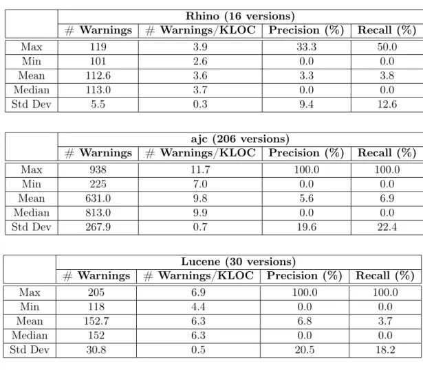
Results: Table 2.6 shows the values measured for recall and precision for the three systems considered in this study. As we can observe, FindBugs reported a large number of warnings/KLOC for the three systems. On average, considering the versions analyzed in the study, FindBugs reported 3.6, 9.8, and 6.3 warnings/KLOC, for Rhino, ajc, and Lucene, respectively. In addition, FindBugs obtained a mean
precision of 3.3%, 5.6%, and 6.8%, respectively. Therefore, the precision results were extremely low. This result indicates that FindBugs raises many warnings in methods that are not changed to fix bugs. Finally, FindBugs yielded an average recall of 3.8%, 6.9%, and 3.7%, for the systems Rhino, ajc, and Lucene, respectively. Such values
indicate that the number of warnings reported by FindBugs is extremely low in the methods effectively changed to fix defects.
Table 2.6: Precision and recall
Rhino (16 versions)
# Warnings # Warnings/KLOC Precision (%) Recall (%)
Max 119 3.9 33.3 50.0
Min 101 2.6 0.0 0.0
Mean 112.6 3.6 3.3 3.8
Median 113.0 3.7 0.0 0.0
Std Dev 5.5 0.3 9.4 12.6
ajc (206 versions)
# Warnings # Warnings/KLOC Precision (%) Recall (%)
Max 938 11.7 100.0 100.0
Min 225 7.0 0.0 0.0
Mean 631.0 9.8 5.6 6.9
Median 813.0 9.9 0.0 0.0
Std Dev 267.9 0.7 19.6 22.4
Lucene (30 versions)
# Warnings # Warnings/KLOC Precision (%) Recall (%)
Max 205 6.9 100.0 100.0
Min 118 4.4 0.0 0.0
Mean 152.7 6.3 6.8 3.7
Median 152 6.3 0.0 0.0
Std Dev 30.8 0.5 20.5 18.2
2.3. Defect Prediction Approaches 25
understand, and remove the field defects evaluated in the study. The main reason for this result is the fact that the warnings reported by FindBugs are based on violations of coding practices (e.g., a class that implements hashCode but does not implement
an equals method) and errors detected by data and control flow analysis (e.g., null
pointer dereference). On the other hand, several field defects are related to logic errors (i.e., errors due to incorrect results). For example, in the specific case of Rhino and
ajc most errors are due to source code in Javascript or AspectJ that is not processed
as expected.
2.3.4
Application of Causality Tests in Software Maintenance
Canfora et al. were one of the first to investigate the use of causality tests in software maintenance [CCPC10]. They proposed the use of the Granger Causality Test to detect change couplings, i.e., software artifacts that are frequently modified together [Gra81]. They claimed that conventional techniques to determine change couplings fail when the changes are not “immediate” but due to subsequential commits. Therefore, they proposed to use the Granger Causality Test to detect whether past changes in an artifact a can help to predict future changes in an artifact b. More specifically, they proposed the use of a hybrid change coupling recommender, obtained by combining Granger and association rules (the conventional technique to detect change coupling). After an study involving four open-source systems, they concluded that their hybrid recommender provides a higher recall than the two techniques alone and a precision in-between the two.
2.3.5
Critical Appraisal on Defect Prediction Approaches
For years, several works were conducted with the purpose of investigating relationships between software metrics and defects [BBM96, DLR10, NB05a, CASV13, GKMS00, Has09]. This fact demonstrates that, despite being an issue is of great importance to the software development process, defect prediction still remains an open problem. In other words, a defect prediction approach that can be adopted by real-world software development projects is still to be reached.
26 Chapter 2. Background
used by defect predictors are linear and logistic regressions. However, linear and lo-gistic regressions do not imply causality [Ful94]. This means that when we identify a linear or logistic relationship between two variables, we can not conclude that one of the variables is the cause of (or directly affects) the other. More specifically, it is well known that regression models cannot filter out spurious correlations [Ful94].
Another issue we want to address concerns the output of the current defect pre-diction models. Currently, this output typically indicates the number or the existence of defects in a component in the future. The availability of this information is im-portant to ensure software quality. However, predicting defects as soon as they are introduced in the source code, e.g., identifying the changes to a class that have more chances to generate defects, can be more useful for developers than simply identifying future occurrences of defects.
Finally, despite the interest and the increasing number of bug finding tools, there is still no consensus on the effective power of these tools to detect defects. Basically, studies aiming to assess the relationship between warnings reported by bug finding tools and bugs also do not consider the idea of causality. Typically, these studies are based on correlation tests such as the Spearman or Pearson correlation test [ACSV10, CASV13]. However, correlation does not imply causality. This means that when we identify a correlation between two variables, we can not conclude that one of the variables is the cause of the other. In other words, spurious correlations may also exist.
To contribute to tackle these issues, we propose in this thesis a defect prediction approach centered on more robust evidences towards causality between source code metrics (as predictors) and the occurrence of defects. The proposed approach differs from the presented studies with respect to three central aspects:
• To the best of our knowledge, the existing defect prediction approaches do not consider the idea of causality between software metrics and defects. Differently, our approach relies on causality tests to infer cause-effect relationships between source code metrics and defects.
• Typically, most studies evaluate their models in a single time frame. In contrast, we evaluated our approach in several life stages of the considered systems.
2.4. Final Remarks 27
2.4
Final Remarks
Chapter 3
Prediction Techniques
In this chapter, we start first by describing the most common modeling techniques used by defect prediction approaches (Section 3.1). In Section 3.2, we present an example of a behavior that can not be captured by standard regressions. Next, we describe a precondition that Granger Causality Test requires the time series to follow and we present and discuss the test (Section 3.3). Finally, we describe and discuss another causality technique (Section 3.4).
3.1
Linear and Logistic Regression
The goal of linear regression is to describe the linear relationship between a dependent variable y and one or more independent variables (x1, x2,· · ·, xk) [Tri06]. For models
with a single variable x, the typical regression equation is expressed in the form y =
b0+b1x and for models involving more variables(x1, x2,· · ·, xk), the general form of a
multiple regression equation is y=b0+b1x1+b2x2 +· · ·+bkxk.
Basically, regression equations can be used for predicting the value of the depen-dent variable, given some particular value of one or more independepen-dent variables. For example, in the context of defect prediction, the dependent variable is the number of defects in the source code of a given class and the independent variables are the values provided by software metrics for this class. Therefore, the ultimate goal is to predict the number of future defects in this class.
Unlike linear regressions, logistic regressions express the relationship between a binary dependent variable (i.e., the dependent variable can take the value 1 with a probability of success π, or the value 0 with probability of failure 1−π) and one or more independent variables (x1, x2,· · ·, xk) [HL00]. The general form of a multiple
logistic regression is based on the following equation:
30 Chapter 3. Prediction Techniques
π(x1, x2,· · ·, xk) =
eb0+b1x1+b2x2+···+bkxk
1 +eb0+b1x1+b2x2+···+bkxk (3.1) whereπ is the probability of the presence of a particular property, thexisare the
inde-pendent variables, and bis are the regression coefficients of the independent variables
that are estimated through the maximization of a likelihood function. In the context of defect prediction, the independent variables are the values provided by software me-trics and the binary dependent variable is the presence or absence of defects in a given class. Therefore, the goal is to discover the probability of this class having a fault.
The most common statistics used to evaluate the quality of linear regressions is called adjustedR2 [Tri06]. An
R2 coefficient measures how well the multiple regression fits the sample data. On the other hand, the quality of multiple logistic regression models is usually evaluated bydeviance (D) [HL00], which has the same role that the residual sum of squares has in linear regression. Basically, a D coefficient denotes a measure of the lack of fit to the data in a logistic regression model.
3.2
Critical Appraisal on Regression
As stated in Section 2.3.1, the most common modeling technique used by defect pdiction approaches is linear and logistic regressions. However, linear and logistic re-gressions do not imply causality [Ful94]. This observation means that when we identify a linear or logistic relationship between two variables, we can not conclude that one of the variables is the cause of (or directly affects) the other variable. In order to illus-trate this issue, we simulated data about software metrics and defects for five classes (Class1, Class2, Class3, Class4, and Class5) of a hypothetical system with 100 versions. Figure 3.1 presents two graphs containing the simulated data. In the graph in the top we plotted the time series with the simulated values of the hypothetical software metric for each class and in the graph in the bottom we plotted the time series with simulated values of the number of defects for each class. As can be observed, an increase in the value of the metric impacted in the number of defects in all the five classes a few time units later. For example, an increase in the value of the metric for the class Class1 from 36 to 136 in the time unit 28 caused an increase in the number of defects from 4 to 9 in the time unit 36.