among Alternative Selective Regimes
Yuheng Huang, Stephen I. Wright, Aneil F. Agrawal*
Department of Ecology & Evolutionary Biology, University of Toronto, Toronto, Ontario, Canada
Abstract
Environmental heterogeneity has been hypothesized to influence levels of genetic variation but the effect of heterogeneity depends on (i) the form of heterogeneity, (ii) whether ecologically relevant or neutral loci are being considered, and (iii) the genetic basis of ecological adaptation. We surveyed genome-wide SNP diversity in replicate experimental Drosophila melanogasterpopulations with equal census sizes that evolved for 42 generations under one of four selection regimes: (i) salt-enriched environment (Salt), (ii) cadmium-enriched environment (Cad), (iii) temporally (Temp) or (iv) spatially (Spatial) variable environments. There was significant differentiation between all pairs of treatments but the greatest differentiation occurred between the two homogenous treatments (CadandSalt). For sites likely under differential ecological selection (and those closely linked to them), the pattern of within-population diversity p followed the expectation from classic antagonistic selection theory:Spatial.Temp.Salt<Cad. However, neutral diversity unlinked to selected sites followed a different pattern:Spatial.Salt<Cad.Temp. As implicated by the latter result, measures ofFSTamong replicate populations within treatments are consistent with differences in effective population sizes among selective regimes despite equal census sizes. Though there are clear changes in the rank order of treatments when contrasting selected and neutral sites with respect to p, the rank ordering of treatments with respect to FST appears reasonably consistent between site categories. These results demonstrate that alternative selective regimes affect within- and among-population diversity differently for different site types.
Citation:Huang Y, Wright SI, Agrawal AF (2014) Genome-Wide Patterns of Genetic Variation within and among Alternative Selective Regimes. PLoS Genet 10(8): e1004527. doi:10.1371/journal.pgen.1004527
Editor:Graham Coop, University of California Davis, United States of America
ReceivedJanuary 4, 2014;AcceptedJune 6, 2014;PublishedAugust 7, 2014
Copyright:ß2014 Huang et al. This is an open-access article distributed under the terms of the Creative Commons Attribution License, which permits unrestricted use, distribution, and reproduction in any medium, provided the original author and source are credited.
Funding:This research was funded by Natural Sciences and Engineering Research Council of Canada through a Discovery Grant to AFA and through the Canada Research Chairs program. The funders had no role in study design, data collection and analysis, decision to publish, or preparation of the manuscript.
Competing Interests:The authors have declared that no competing interests exist.
* Email: [email protected]
Introduction
Patterns of genetic variation have several major consequences for evolution. First, the amount and type of genetic variation in fitness mediate a population’s ability to adapt to selection pressures. Second, the nature of genetic variation determines the fitness consequences of different types of reproduction (e.g., sexual versus asexual reproduc-tion, inbreeding versus outbreeding, random mating versus mate choice), and can therefore be a major cause of selection on reproductive traits. Third, the amount of neutral variation determines the rate at which populations diverge by drift. But what factors shape variation within populations and create differences in levels of variation among them? This is one of the central questions in evolutionary biology [1,2]. Here we examine how different selective regimes alter patterns of variation across the genome.
When considering genetic variation in fitness, selection must be a major determinant, but the relative importance of different types of selection is unknown. One possibility is that most genetic variation in fitness is due to the constant input of new deleterious mutations balanced by the removal of such variants by negative selection. While mutation-selection balance undoubtedly contributes to variation in fitness, several authors have argued that this model is unable to fully account for empirical observations [3,4]. The alternative is that some form of balancing selection (e.g., negative frequency-dependent selection, antagonistic pleiotropy, environmental heterogeneity) actively maintains multiple alleles at selected sites.
In theoretical models, the form of selection is imposed by assumption, but, in nature, selection is a consequence of the environment. A common feature of natural environments is that they change over time and space. Here we use experimental evolution to ask how this key feature affects genome-wide patterns of selected and neutral variation. Below we review several simplistic predictions for selected sites but emphasize that these are based on alternative assumptions regarding how environmental heterogene-ity changes selection and ignore the effects of linked loci.
Classic theory [5,6] predicts that genetic variation at selected sites can be maintained by environmental heterogeneity if alternative alleles are favoured in different environments (environmentally antagonistic selection, EAS). However, the type of heterogeneity is important; the conditions for a protected polymorphism through balancing selection are more restrictive with temporal heterogeneity than spatial heterogeneity [6,7]. From this, we expect to find the most genetic variation for fitness in spatially heterogeneous populations, somewhat less in temporally heterogeneous popula-tions, and the least variation in populations evolving in a constant environment (i.e.,VSpatial.VTemp.VConst).
both environments, conditionally neutral alleles experience half as much directional selection. Therefore, the heterogeneous regimes are expected to harbor levels of genetic variation for this locus intermediate to that in populations maintained in A or B alone (i.e.,VConst_A.VSpatial.VTemp.VConst_B). However, if we consider
multiple loci and assume that some experience selection only in A and others only in B, then the average amount of variation across these loci might be lowest in the heterogeneous populations where variation should be purged eventually from both types of loci (i.e., VConst_A,VConst_B.VSpatial.VTemp).
Rather than favoring the phenotypes specialized for either A or B, a third possibility is that heterogeneous environments select for a distinct phenotype (e.g., a robust generalist rather than the maintenance of multiple specialists). In this case, populations from heterogeneous environments would not be genetically intermedi-ate between populations from alternative constant environments; rather, they might be as genetically distinct from the homo-genously selected populations as the homohomo-genously selected populations are from one another. Under this scenario, there is no reason to expect levels of variation to differ among selective regimes.
While some sites experience different selection between different environments or between homogeneous versus heterogeneous regimes, most sites will be uniformly selected across environments or neutral in both environments. However, variation at such sites will be influenced by changes in selection at other sites in the genome due to genetic hitchhiking (linkage effect). The extent of this influence will depend on the number of differentially selected sites, the strength, form and timescale of selection on these other sites, as well as their distribution across the genome and the recombination rates between them [8–10].
A number of important experimental studies have examined the effect of environmental heterogeneity on genetic variance (quan-titative genetic variation: [11–17]; allozyme heterozygosity: [18–
20]). The findings from these studies are quite variable and often there are few significant differences between treatments. Logistical constraints have limited past studies to either quantitative genetic analysis of a small number of traits or diversity measures from a handful molecular markers. It is impossible to know whether unmeasured traits or loci were similarly affected. An additional challenge in interpreting past results is that it is often unclear whether the traits or loci being studied are under differential selection between environments or even closely related to fitness. High-throughput sequencing offers new opportunities to re-examine this issue. This technique has been applied to study the genetic basis of selection response in experimental populations (e.g., [21–24]). We applied this technology to replicated experi-mental populations ofDrosophila melanogasterthat evolved under different selective regimes. Twenty replicate populations were established from a cross between an ancestral lab population adapted to a salt-enriched larval environment (‘‘Ancestral Salt,’’ AS) and an ancestral lab population adapted to a cadmium-enriched larval environment (‘‘Ancestral Cad,’’ AC). These 20 replicates (N= 448 per population) were divided equally among four treatments: two constant treatments in either salt- (Salt) or cadmium-enriched (Cad) larval environments, a temporally heterogeneous treatment (Temp) in which populations were switched between each generation to the alternate environment, and a spatially heterogeneous treatment (Spatial) in which the population was split between the two environments but surviving adults were mixed with equal number from the two environments before egg-laying for next generation. After ,20 generations,
Long et al [25] found striking differences across treatments in inbreeding depression, suggesting important shifts in patterns of variation within populations among treatments.
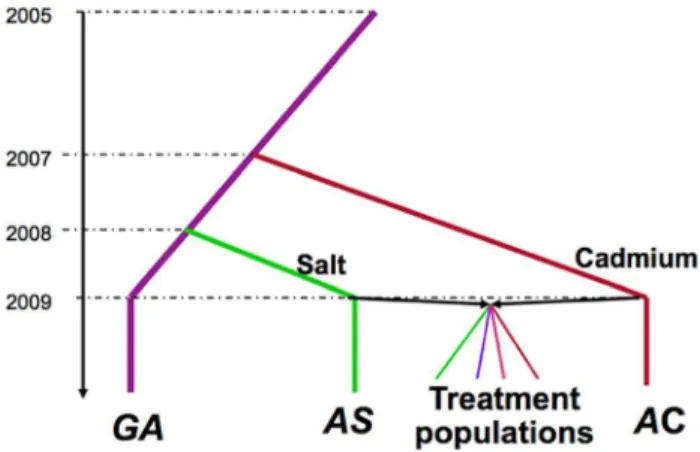
At generation 42, we performed pooled re-sequencing of each of the 20 populations, the two environmentally specialized ancestral populations (AS and AC), as well as the lab source population (‘‘Grand Ancestor’’,GA) from whichASandACwere derived (see Figure 1 for relationship among populations). We first examine genetic differentiation among treatments and identify candidate sites under differential selection. We then compare levels of within-population variation among treatments. There are major
differ-Figure 1. Selection history of the experimental populations.
The Grand Ancestor population (GA) was maintained in benign laboratory conditions, and was used to initiate populations maintained on salt-enriched media (AS) or cadmium-enriched media (AC). The treatment populations were produced by crossing two ancestral populationAS andAC. There are 5 replicate populations of each of the four treatments (not illustrated).
doi:10.1371/journal.pgen.1004527.g001
Author Summary
ences in levels of variation among treatments and these patterns change between neutral and putatively selected sites.
Results
Differentiation for environment-specific survival
We tested the survival of flies from all replicate populations in both environments. Contrasting the two constant treatments, we found the expected patterns of local adaptation, i.e., Cad populations had higher survival thanSaltpopulations when tested in cadmium but the reverse was true in salt (Figure 2). In the salt (cadmium) environment, the survival rates of flies from heteroge-neous treatments were considerably higher than flies from Cad (Salt) treatment, indicating populations perform poorly when tested in an environment to which they lack selective exposure. These results are qualitatively similar to those reported by Long et al [25] from an earlier time point (,generation 20).
Allele frequency differentiation between salt and cadmium environments
In addition to measuring the differentiation in survival, we measured differentiation in the frequencies of single nucleotide polymorphisms (SNPs) between the Salt treatment and Cad treatment. After read mapping and filtering for map and base quality, we had a mean coverage among populations of,17.5 fold
for euchromatic regions.
To maximize our power in examining differentiation that occurs between populations evolving in the two extreme environ-ments, we compared allele frequencies in the Ancestral Salt (AS) and the five Salt populations with allele frequencies in the Ancestral Cadmium (AC) and the five Cad populations. To identify SNPs, we screened for sites in euchromatic regions that are $5-fold coverage in all of these populations. We kept only those sites where the initial diversity (pini) was not too low,
specificallypini= 2pini*(12pini).5%, where piniis the estimated
frequency of the minor allele pooling across the Ancestral Salt (AS) and Ancestral Cad (AC) populations. After applying these screens, there were,2*106sites for testing differentiation; we refer to these
sites as the ‘‘a-sites’’. To maximize our statistical power, we considered allele frequency estimates from the five replicateSalt populations and the Ancestral Salt (AS) population as replicates for a ‘‘salt’’ treatment and the estimates from the five replicate Cad
populations and the Ancestral Cad (AC) as replicates for a ‘‘cadmium’’ treatment and then used a screen for allele frequency differentiation between treatments based on the Cochran-Mantel-Haenszel test (CMH) [26]. A total of 123,291 sites passed our screen for significant differentiation with false discovery rate = 0.001%; we refer to these as the ‘‘b-sites’’. Because differentiation likely occurs from common variants, we expect the variation in the Grand Ancestor population to be greater at b-sites than othera-sites. Indeed, diversity is ,20% greater (i.e., pGA,b-sites= 0.290;pGA, othera-sites= 0.246).
To evaluate the potential for false positives due to sampling error, allele frequency estimation error or genetic drift, we randomly assigned half of our cadmium populations as well as half of our salt populations to pseudo-treatment ‘‘A’’ and the remaining cadmium and salt populations to pseudo-treatment ‘‘B’’. We then performed the same analysis looking for differen-tiation between ‘‘A’’ and ‘‘B’’. We repeated this process for 15 randomly chosen combinations. Among these combinations, we found the mean number of sites that passed the same criteria above was 93, with the highest number 349. Thus, we expect the majority of the ,123000 significant differentiated sites are not
false positives in a statistical sense.
Nonetheless, it is highly improbable that,123000 b-sites are
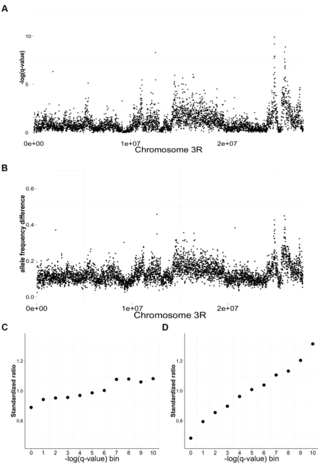
direct targets of differential selection. Much of the differentiation is likely the result of linkage effects. In the most extreme situation, there could be just one or two selected sites per chromosome and all the other sites could differentiate because of linkage. However, there are several observations that would not be expected if linkage effects were massive and there were only a few true targets of selection: (1.1) Rather than observing a single large block of differentiation, we observe numerous distinct peaks of differenti-ation across each chromosome (plotted as non-overlapping sliding windows Figure 3A–B, Supplementary Information S1A and Figure S1 for whole genome); (1.2) Among the most strongly significantly differentiated sites, there is an enrichment of (i) intragenic to intergenic sites, and (ii) coding to non-coding intragenic sites (Figure 3C–D). (There is no enrichment of nonsynonymous sites relative to 4-fold degenerate sites suggesting strong linkage effects at this small scale; more details in Supplementary Information S1B and Figure S2); (1.3) Differen-tiation is not random with respect to gene function, rather certain classes of genes (Gene Ontology) show enrichment, including those
Figure 2. Mean survival in cadmium (A) or salt (B) environment.Each point represents the mean survival of,140 full-sib families for each
involved with protein metabolic process and peptide activity (Supplementary Information S1C and Table S1). Moreover, similar functional categories are identified when gene enrichment tests are performed separately for the two major autosomes (Table S1). In addition, some of our differentiated genes had been identified in previous functional studies of cadmium and salt resistance (e.g., MtnB, MTF-1 for cadmium resistance [27,28] and CG6484, sug, Sik3, CrebA, Crtc for salt resistance [29,30]).
Other patterns suggest that linkage effects are contributing to differentiation but on a scale much smaller than the whole chromosomes: (2.1) The b-sites are strongly (and significantly) clustered relative to the distribution of a sites across genome. However, the level of clustering declines rapidly within 5000 bp, though a lower level of clustering extends much further (Supplementary Information S2A and Figure S3). The pattern of clustering remains similar after controlling for initial diversity in the GA population, which could affect the likelihood of differentiation and the power to detect it (not shown); (2.2)FST
between salt and cadmium populations is very high near focal differentiated sites but declines rapidly within the first 500–1000 base pairs (Supplementary Information S2B and Figure S4); (2.3) The linkage disequilibrium (LD) within the paired-end reads (2*100 bp) declines relatively rapidly within the first 100 bp from 0.7 to about 0.4 (Supplementary Information S2C and Figure S5). These patterns remain similar when we only consider the regions that containb-sites.
To assay the potential impact of inversions on genetic differentiation and as a source of linkage disequilibria, we used previously identified inversion-specific SNP markers [31] to estimate the inversion frequency in our populations (Supplemen-tary Information S2D). The frequency of all potential inversions across the six populations in constant cadmium and six populations in constant salt environment are lower than 5%. Given the average allele frequency differentiation ofb-sites is,0.4
(Tables S2, S3 and Supplementary Information S3), inversions are unlikely to play a major role. Further, for the two major autosomes, on average, the relative abundance of theb-sites and level of LD do not seem to be elevated in regions of commonly segregating inversions (Tables S4, S5 and Supplementary Infor-mation S5). As the linked selection is expected to be stronger in low recombination regions, we calculated the number and proportion of b-sites and a-sites in each of these regions (Table S6). Consistent with the prediction of greater effects of linked selection, there is a higher proportion of significant sites toa-sites in low recombination regions than high recombination regions (7.6% vs 5.4%, the difference is caused by autosome 2).
Recent papers [32–34] suggest that ‘‘evolve & re-sequence’’ studies have limited power to identify true targets of selection and our observation of clustering ofb-sites and LD is consistent with those concerns. However, for our purposes, it is not essential to identify the true targets, rather our purpose is to demonstrate that the two alternative habitats cause genetic differentiation. None-theless, such differentiation is more meaningful if it is not due to selection on only one or two sites. Taken together, the results above suggest that the b-sites are enriched for true targets of selection but that many of theb-sites are differentiated because of linked selection. Linkage effects are likely strong but the patterns reported above (e.g., enrichment of significant sites in coding regions as well as gene ontology enrichment) do not seem consistent with selection on only a few sites. However, we emphasize that we cannot identify true targets of selection or reliably estimate whether the true number of targets is in the tens, hundreds, or more. We conclude only that the salt and cadmium environments cause populations to diverge genetically and that,
though much of the differentiation may be due to linkage effects, there are likely multiple targets of selection.
Pairwise genetic differentiation between selective regimes
After establishing the high degree of differentiation across the genome between the two constant environments, we examined the level of differentiation between all other pairs of treatments. In the preceding section we compared the salt and cadmium environ-ments and included the ancestral populations to maximize power for findingb-sites. In this section, we use only the five replicate populations within each experimental selection regime (the ancestral populations are not considered) so that we have similar power to examine differentiation between all pairs of treatments (e.g.,Saltvs.Cad;Tempvs.Spatial). The number of significantly differentiated sites between each pair of treatments is shown in Table 1. The number of differentiated sites between the two homogenous treatments (CadandSalt) is much greater than the numbers between any pair of homogeneous and heterogeneous treatments (e.g., Cad and Spatial). The two heterogeneous treatments (Spatial and Temp), where populations experience both selective agents, have many fewer differentiated sites than any other pair of treatments. The numbers of genes with significantly differentiated sites shows the same relationship among treatment pairs (Table S7).
As an alternative approach to comparing treatments, we measured the correlation of allele frequencies between different pairs of treatments using the sites that are likely under differential selection. To avoid bias in comparing treatments, we identified sites that were significantly differentiated in allele frequencies betweenASandAC, the direct ancestors of all treatments (using Fisher’s exact test with q-value,0.001). Because a correlation in allele frequency will arise simply from variance among sites in initial allele frequency, we calculated a ‘standardized’ correlation of allele frequency between each treatment pairs by using the correlation for differentially selected sites minus the correlation for non-differentiated control sites (details in Supplementary Infor-mation S3 and Table S8). We found the standardized correlation between theSaltandCadtreatments is significantly negative, and more negative than the correlation between any other pair of treatments. The negative correlation possibly suggests that the most strongly favored alleles in one environment are the most strongly disfavored in the other environment, indicating the operation of environmentally antagonistic selection (EAS). On the other hand,TempandSpatialtreatments have the most positive correlation, which is consistent with the differentially selected sites experiencing similar selection pressures between the two hetero-geneous treatments (Supplementary Information S3 and Table S8).
Molecular diversity in alternative selective regimes
Our major goal is to compare the molecular variation among different treatments. First, we compared the genome-wide average diversity (p) among treatments. We used non-overlapping sliding windows to calculate Tajima’spover,95% of the euchromatic region of the genome for which we have sufficient coverage in all populations [35,36]. The mean p across the genome for each population is shown in Figure 4. There is significant variation inp among treatments (F3,16= 9.68, P= 0.0007); the genome-wide
Figure 3. Differentiation between salt and cadmium populations.Sliding-window (5 kb non-overlapping) plots of differentiation along chromosome 3R: the average -log(q-value) from the CMH test (A) and the average difference in mean allele frequency (B) between the salt and cadmium populations. For each environment, the data are calculated based on the environment-specific ancestor and the five replicate populations. The ratio of the number of genic to intergenic sites (C) and the ratio of the number of coding sites to intronic sites (D) in different -log(q-value) bins using data from the whole genome. To compare the magnitude of the ratios for different functional catergories, the ratios are standardized around 1 by dividing the mean ratio among the 11 bins. Strong significance corresponds to larger values of -log(q-value).
genome-wide averages belies more interesting patterns that emerge at a finer scale.
The prediction ofVSpatial.VTemp.VConstis for antagonistically
selected sites, but many of the variable sites are likely neutral (or effectively neutral). To better test the prediction, we attempted to identify the sites that are likely under differential selection between the salt and cadmium environments. For this section, we want to identify potential targets of differential ecological selection using only the data from the two ancestral populations (AC and AS). This is necessary to avoid biasing tests comparing among selective treatments. To do so, we applied a different screen than used in the earlier sections. First, to increase the accuracy of the estimation of allele frequency, we screened sites that have$15-fold coverage in both ancestral populations and havepini.5% (estimated from the average allele frequency in theACandAS). Also, we screened for the sites that have$10-fold coverage for all of the 20 treatment
populations. In total, we had 769,924 SNPs for this analysis; we refer to these as the ‘‘x-sites’’.
We calculated the degree of differentiation in allele frequency between the two ancestral source populationsASandACfor all of the x-sites, i.e., d= |pAS2pAC|. Sites under environmentally
antagonistic selection will tend to have highdvalues. Because all treatments were created equally fromASandAC, there should be no initial differences inpamong treatments for any given level of d. However, differences inpamong treatments should develop due to treatment-specific selection, and the nature of these differences is expected to vary withd (i.e., selection is likely similar across treatments for lowdsites whereas high dsites likely experience very different selection in different treatments).
To illustrate how the variance changes as we move from neutral sites to sites putatively under differential selection, we calculatedp across the complete range of differentiation (d) values (Figure 5A). For all treatments,p is lower for weakly differentiated sites than strongly differentiated sites. This pattern is expected simply because the experimental populations were founded by crossing ACandAS; thus, sites that are strongly differentiated betweenAC and AS will start off as highly polymorphic within each experimental population. More interestingly, the rank order of the treatments with respect to diversity changes from weakly differentiated sites (pSpatial.pSalt<pCad.pTemp for d,0.3) to
highly differentiated ones (pSpatial.pTemp.pSalt<pCadford.0.7).
To more clearly see the effect of selection, it is helpful to comparep between weakly and strongly differentiated sites that have similar levels of initial diversity. To do so, we re-examined the data using only those sites that have high initial diversity (pini.
0.4, wherepini= 2pini(12pini) andpini=K(pAS+pAC)). Using these
sites, the relationship ofptodis very different for heterogeneous treatments than for homogeneous treatments (Figure 5B). In the constant selection environments p declines with d, as expected under directional selection. In contrast,pis relatively high at both low and high values ofdfor heterogeneous treatments.
When we compare levels of diversity among treatments using thex-sites with high initial diversity (pini.0.4), we find different patterns for sites that are weakly or strongly differentiated between the ancestral founding populations. For the putatively ‘neutral’ sites (arbitrarily designated asd,0.3), we find significant variation in p among treatments (F3,16= 5.8, P= 0.007; Figure 5C) with
treatments ranked as pSpatial.pCad.pSalt.pTemp. There is also
significant variation inpamong treatments for the sites likely to be under differential selection (d.0.7, F3,16= 19.5, P= 1.36E25;
Figure 5D) but the order is pSpatial.pTemp.pSalt.pCad. These
differences in diversity are not driven by the potential effect of inversions (which seem to be very rare in our population, Table S2). After excluding the x-sites located within inversion regions, Table 1.The number of highly differentiated sites between each pair of treatments.
Cad Temp Spatial
Salt 90661 9427 6456
Cad 14528 3528
Temp 488
For each pair of treatments, we performed CMH tests on each site using the five replicate populations from each treatment. For theCadvsSaltcomparison here we used only the five replicate populations for each treatment; for the main analysis discussed in the text we also included the ancestral populations of each treatment (AC
andAS). We did five different ways of pairings for the tests. The q-value was calculated from the p-value for each pairing in the CMH test and then transformed by the ‘‘BY’’ method. Then we used q-value cutoff equals 1025to pick up the significant sites that pass this cutoff for all five ways of pairings. For the Salt-Cad pairs in the Table, 93.8% of the significant sites (90661) are found in theb-sites (123291) and forTemp-Spatial, it is just 13.7% of them (488). ForSalt-Temp,Salt-Spatial,Cad-Temp, Cad-Spatialpairs, there are 71.8%, 82.8%, 64.3% and 78.2% of their own significant sites found in theb-sites (sixSalt-sixCad) respectively.
doi:10.1371/journal.pgen.1004527.t001
Figure 4. Average diversity (p) within experimental popula-tions across the genome.Each point represents the meanpacross the common sliding windows (including non-variable sites) for each population. Though ancestral populations are shown for reference, we are primarily interested in the mean diversity (p) among the four treatments that were created by crossingACandAS. There is significant variation among the four treatments (F3,16= 9.68,P= 0.0007). The ‘‘b’’
group is significantly higher than the ‘‘a’’ group based on ANOVA Tukey HSD test. Spatial has significantly higher diversity than the Temp
(Padj= 0.0006, Tukey HSD), the Salt (Padj= 0.026) and the Cad
(Padj= 0.0036).
the diversity patterns are qualitatively similar (Supplementary Information S4 and Figure S6)
Divergence among replicates within treatments
The reduced level of diversity at ‘neutral’ sites within theTemp treatment suggests that populations in this treatment have the lowest Ne. Drift should not only reduce diversity within populations but
also cause divergence among populations. To test the latter, we examined FST among the five replicate populations within each
treatment. For this analysis, we used ‘neutral’ sites passing a minimum coverage and initial diversity thresholds (i.e., thex-sites above withpini.0.4 andd,0.3). As expected,FSTwas higher for X
chromosome sites than autosomes in all four treatments, (X FST= 0.1566007; autosome FST= 0.1396008; t=23.87, df = 3, P= 0.026). We then comparedFST among treatments using five
regions of the genome that are approximately recombinationally independent: the X chromosome, and the left and right ends of each of the two autosomes (Figure 6A). There was significant variation among treatments inFSTvalues (F3,16= 6.72,P= 0.004), with
post-hoc tests showing this was primarily due to elevatedFSTin theTemp
treatment, consistent with a lowerNefor this treatment. It is worth
noting that the treatments do not differ in expected total heter-ozygosity (HT) for these sites (F3,16= 1.02, P= 0.41, Figure 6C),
which can be a misleading cause of differences inFST[37]. Figure 5. Meanpwithin treatments as function of differentiation (d) between the ancestral source populations (ACandAS).(A) and
(B) The averagepacross different levels of ancestral differentiation for (A) allx-site SNPs or (B) only thosex-site SNPs that have high initial diversity (pini.0.4). Thex-axis is the allele frequency difference between ancestral populations,d= |pAC2pAS|. Error bars represent the standard error among
the five replicates for each treatment. (C) and (D) Comparison among treatments in averagepfor sites that have high initial diversity (pini.0.4) using
sites with (C) weak ancestral differentiation (d,0.3) or (D) strong ancestral differentiation (d.0.7). For the weakly differentiated sites (C),Spatialhas significantly higher diversity than theTemp(Padj= 0.006, Tukey HSD) and theSalt(Padj= 0.028). For the highly differentiated sites (D), bothSpatialand
Temptreatments have significantly higher diversity than the two constant treatments (Padj,0.03 between any a & b pairs).
The equivalent comparison of within-treatmentFSTfor sites likely
to be under differential ecological selection (d.0.7) does not show significant differences among treatments (F3,16= 1.16, P= 0.35,
Figure 6B) but the patterns are qualitatively similar to the ‘neutral’ sites.HTdoes not vary significantly among treatments (F3,16= 1.59,
P= 0.23; Figure 6D), though point estimates of averageHTare higher
in the heterogeneous treatments than the homogeneous ones. It is worth noting that while both heterogeneous treatments have elevated
HTvalues, theTemptreatment has the highestFSTvalue whereas the Spatialhas the lowest. These patterns suggest the differences inNe
betweenSpatialandTempaffect differentiation among replicates even at sites under selection (or those linked to them). Based on the low within-population diversity of the constant environments (Figure 5B), we might have expected elevatedFSTfor these treatments. However
this is not the case and may be attributable to the ‘selected’ sites experiencing stronger net selection in these treatments.
Figure 6.FSTvalues for each treatment in different regions.We screened for thex-sites above withpini.0.4 and divided them into five
recombinationally independent regions of the genome. For weakly differentiated sites (d,0.3, Figure 6A), There is significant variation among treatments in FST values with Temp being highest among them (F3,16= 6.72, P= 0.0038). The Temp has significantly higherFST than Spatial
(Padj= 0.002). The difference betweenTempand the two constant treatments are marginally non-significant (Tempvs.Salt:Padj= 0.084;Tempvs.Cad:
Padj= 0.087). For highly differentiated sites (d.0.7, Figure 6B), theFSTvalues do not significantly differ among treatments (F3,16= 1.16,P= 0.35). For
both weakly and highly differentiated sites, the treatments do not differ in expected total heterozygosity (HT) (F3,16= 1.02, P= 0.41, Figure 6C;
F3,16= 1.59,P= 0.23, Figure 6D).
Discussion
In nature, many populations experience environments that are heterogeneous in space or time. Though our experimental populations differ from natural populations in a number of ways (population size, time scale of adaptation, etc.), our study provides insight into how alternative selective regimes affect genome-wide patterns of molecular diversity in an experimentally simplified setting. In our study, we used two environments that cause populations to diverge with respect to environment-specific survival (Figure 2) as well as allele frequency at numerous SNPs (Figure 3). Though we are unable to determine the number or identity of true genetic targets of differential ecological selection, our analyses suggest that there are likely to be more than one or two per chromosome.
For variants that are likely under differential selection between cadmium and salt environments (or statistically linked to such sites), the diversity patterns are consistent with the classic theoretical prediction: VSpatial.VTemp.VConst (Figure 5D). In
contrast, the pattern of diversity of other sites is different: VSpatial.VConst.VTemp (Figures 4 and 5C). In other words, the
rank order of treatments with respect to genetic diversity differs between ecologically selected sites and other sites. Our classifica-tion of ‘selected’ sites likely includes many neutral sites that are statistically linked to true targets of selection, due to physical linkage or, perhaps more importantly, through admixture or stochastic association from the founding of these populations [32– 34]. However, for our purposes of studying diversity, such sites behave similarly to sites under differential ecological selection because of their statistical association with true targets.
The difference in the rank order of treatments between ‘selected’ and other sites may help to reconcile inconsistencies among classic studies [11–20] attempting to assess how alternative selective regimes affect genetic variance in phenotypes or genetic markers. In most of those studies, phenotypes or genetic markers had unknown relationships to experimentally imposed ecological differences in selection. Even in cases where measured phenotypes or markers are unlikely to have any true ecological effect, they might have been statistically linked to genes that did, making it difficult to interpret such results. By categorizing sites based on information from the ancestral populations, we found very different patterns of variation among our experimental treatments for different categories of sites within the context of a single study. The difference in the rank order of treatments between ‘selected’ and other sites seems to occur primarily because of how selection affects diversity in homogeneous environments. Focusing on a set of sites that should have similar initial levels of diversity (Figures 5B–D), we found that diversity levels in the two heterogeneous treatments were similar between ‘selected’ and ‘neutral’ sites, but with diversity inTempbeing consistently,6% lower than in the Spatial treatment. In contrast, diversity in homogeneous treatments is ,14% lower than the Spatial
treatment for ‘selected’ sites but only,4% lower for neutral sites.
In simplistic simulations with environmentally antagonistic alleles (Supplementary Information S5 and Figure S7), we were able to qualitatively reproduce these patterns by considering physical linkage to selected sites. In constant environments, neutral diversity was reduced in simulations where the neutral site was closer to selected targets compared to simulations where the recombination distance was greater. For simulated populations evolving in spatially heterogeneous environments, physical linkage to selected sites had only weak effect on neutral diversity, unless selection was strong. With temporal heterogeneity there was no noticeable effect of physical linkage on neutral diversity.
Spatial heterogeneity can result in balancing selection. Previous theoretical studies have shown that balancing selection is expected to increase neutral diversity, but only at sites closely linked to the targets of balancing selection [38]. In contrast, Barton [39] showed that temporally fluctuating selection is expected to reduce neutral variation across the genome (see also [40,41]). When linkage is loose relative to selection, the drift experienced by neutral sites will be increased by an amount proportional to the enhanced amount of additive genetic variation maintained by fluctuating selection. For more closely linked sites, the loss of diversity can be much more extreme if allele frequencies at the selected loci are oscillating between extreme values. Fluctuating selection is only expected to increase diversity for sites with extremely tight linkage and only when time scales are very long [39]. The latter effect results from the build up of mutations during the longer coalescent times of sites linked to targets of balancing selection relative to those sites that are unlinked. However, if fluctuating selection is applied to standing variation for a short period, as in our simulations and experiment, there appears to be little relationship between physical linkage to selected sites and diversity.
The patterns in the simulations are qualitatively similar to those in our data if we assume our strongly differentiated sites (d.0.7; Figure 5D) are more tightly linked to true selected targets than are our ‘neutral’ sites (d,0.3). Another approach to examining the importance of linkage is to compare diversity in regions of high versus low recombination. If we assume that neutral sites will tend to be more tightly linked to a true target in the regions of low versus high recombination, then there should be differences in the diversity between low and high recombination regions but these differences should vary among treatments. Controlling for initial diversity of sites among regions, there is significantly less variation in low recombination regions than in high recombination regions in theCad (Supplementary Information S6, Figures S8 and S9, Table S9), as expected. However, diversity does not differ between high and low recombination regions in the other treatments. This lack of a difference is reasonably consistent with the predictions of our simulations (Figure S7) and our analysis based on d (Figure 5B) for the two heterogeneous treatments but not forSalt. The contrast between high and low recombination regions used here is a crude comparison because (i) the distribution of true selected targets across these regions is unknown and (ii) even the ‘‘low’’ recombination regions likely include many neutral sites that have low degree of linkage from selected sites.
Differential selection between environments could take two qualitatively different, but not mutually exclusive, forms: environ-mentally antagonistic selection (EAS) and conditional neutrality (CN). This experiment was not designed to distinguish between them but we can consider the observed patterns in light of these alternatives. For sites strongly differentiated between the ancestral populations (ASandAC), the diversity pattern in the experimental populations is consistent with the prediction from the antagonistic selection model. After controlling for initial diversity, diversity is reduced for putatively selected sites compared to other sites in the constant selection treatments but not in the heterogeneous treatments (Figure 5B). Under CN we would expect the heteroge-neous environments to show a decline in diversity for selected sites, albeit a less severe decline than in the constant environments. In contrast, the diversity increases for sites expected to be more strongly selected (i.e.,pincreases withdford.0.6, Figure 5B), suggestive of EAS. An additional observation suggestive of antagonistic selection is the negative correlation in allele frequency betweenSaltandCad treatments (Supplementary Information S3 and Table S8).
dip in diversity seen in Figure 5B for both heterogeneous treatments for sites with intermediate levels of divergence between the two ancestral populations (0.4,d,0.6). One possible expla-nation emerges from considering the type of sites likely to be found at different levels ofd(whered= |pAC2pAS|). Low values ofdwill
be enriched for sites that are neutral or uniformly selected across environments whereas high values of d will be enriched for environmentally antagonistically selected sites. Compared to EAS sites, conditionally neutral sites will tend to show less differenti-ation between the two ancestral populdifferenti-ations (i.e., intermediate values ofd) because they are selected in only one ancestor and are neutral in the other. In the heterogeneous habitats, variation from such sites is expected to be eliminated because one allele is deleterious some of the time and never advantageous. This would explain the reduced diversity for sites with intermediate values ofd compared to neutral sites (lowdsites).
Conditionally neutral alleles should show evidence of being selected in one environment but not the other. We cannot rigorously test for this but, as a first approximation, we can consider the fraction of sites that are differentiated between environments but also show little change in allele frequency from the ancestral state in one of the two habitats. Of sites significantly differentiated between salt and cadmium (b-sites), ,5% (6620/
123291) could be classified as possibly neutral in cadmium based on showing low differentiation between the Ancestral Cadmium population and theGrand Ancestor(|pAC2pGA|,0.1) as well as
low differentiation between the five replicateCadpopulations and the initial allele frequency (|pCad2pini|,0.1, where pini= (pAC+ pAS)/2). Similarly, ,6% (7498/123291) could be classified as possibly neutral in salt. By thisad hoccategorization, only,11%
of significantly differentiated sites show a pattern consistent with CN.
The discussion above has focused on scenarios (EAS and CN) where selection in heterogeneous environments is intermediate to that of the two homogeneous environments. However, environ-mental heterogeneity may select for properties not favoured in either constant environment. We see some evidence suggestive of unique sites being favoured by heterogeneity. Among the several thousands of significantly differentiated sites between any pair of heterogeneous and homogeneous treatments (Table 1), about 20% to 35% of such sites are different from the sites differentiated betweenCadandSalttreatments. This means that the divergence of a heterogeneous treatment from a homogeneous treatment is not a simple subset of the divergence between alternative homogenous treatments, suggesting that some sites respond specifically to heterogeneity. Heterogeneity may favor a generalist or plastic genotype (rather than a mix of specialists) and this is thought to be more likely with temporal than spatial heterogeneity [42]. Relative to the Spatialtreatment, the Temp treatment has more significantly differentiated sites from the constant treatments (23745 vs. 9920) and these sites are less likely to be differentiated between the two constant treatments (9147/23745 = 39% of sites differentiated betweenTempand the constant treatments are not differentiated between the two constant treatments; 2278/ 9920 = 23% forSpatial;x2= 754.7179, df = 1, p-value,2.2e-16). Understanding the mechanisms maintaining genetic variation is a classic pursuit of evolutionary biology. Environmental heteroge-neity has long been postulated to sustain elevated levels of variation through antagonistic pleiotropy between environments, which can result in balancing selection especially if heterogeneity is spatial rather than temporal. However, rather than antagonism, different loci may be selected in each environment (i.e., conditional neutrality). Further, heterogeneity may select for alleles different from those favored in either single habitat (e.g.,
generalist genotype rather than a mixture of specialists). These three distinct, but not mutually exclusive, possibilities create uncertainty in how environmental heterogeneity will affect genetic variation. Although there is indirect evidence of each of these genetic possibilities in our data, the major patterns are most consistent with environmental antagonism. However, even con-sideration of EAS alone does not lead to a single prediction because the effect of environmental heterogeneity on neutral sites depends on their linkage to selected sites.
Although the patterns of diversity among treatments are most consistent with the prediction from EAS, it is likely that some populations are not at equilibrium and these patterns could change over time. For example, we expect CN sites specific to each environment would lose variation in heterogeneous treatments but the rate of loss would be slower than in the appropriate homogenous environment where they experience constant selec-tion. Thus, the relative contributions of CN and EAS sites to diversity will change over time and at different rates across treatments. Given that the current patterns appear to be dominated by EAS and that the contribution of CN is expected to decline over time, it seems unlikely that the patterns would change dramatically through this effect. Nonetheless, it would be ideal to re-sequence these populations at several time points in the future. From the changes in allele frequencies during a time series, we could gain a better sense the effects of environmental heterogeneity on the genetic variation and how these change over time.
This experiment serves as a case study of the effects of environmental heterogeneity on genome-wide variation in a simplified setting, demonstrating distinct differences between environmental heterogeneity in space versus time and between sites likely to be closely linked or not to sites under differential ecological selection (Figure 5). Yet this experiment is only a single test of environmental heterogeneity at one time point; different environments, different spatial or temporal scales of heterogeneity, or different organisms could yield different patterns because the results will depend on the genetic basis of adaptation and the nature of selection [43]. A recent study in yeast suggests that antagonistic effects may be common [44]. But other field studies in plants found that patterns of conditional neutrality are more common [45,46]. A recent study in Brassicaceae quantified the proportion of conditional neutral and EAS QTLs across genome and found that conditional neutrality is more common than EAS (8% vs. 3% of the genome, [47]). The ultimate challenge remains to determine how environmental variation affects patterns of diversity and quantitative genetic variation in nature in different organisms (e.g., [48]). Because the constraints of real systems make it difficult to cleanly test these effects in nature, experimental evolution provides a helpful step towards testing the key principles [49].
Methods
History of selection populations
The selective histories of all populations we used are illustrated in Figure 1. A population ofDrosophila melanogasterwas collected in the Similkameen Valley, British Columbia in 2005 and maintained in regular benign conditions at large size (,2000–
4000 adults, by S. Yeaman); we refer to this population as the ‘‘Grand Ancestor’’ (GA). In July 2007, a subset of flies from theGA population was used to initiate 12 replicate populations (each has
,1000 adults) maintained in a cadmium-enriched environment
environment (with a population size of,2000 adults), we refer to
this as the ‘‘Ancestral Cadmium’’ (AC) population. In August 2008, a subset of flies from the GA population was used to initiate a population (with a population size of,2000 adults) maintained in
a salt-enriched environment (by A. Wang); we call this the ‘‘Ancestral Salt’’ (AS) population. During the adaptive history, the amount of cadmium and salt in the environments were progressively increased, reaching 75mg/ml and 29 mg/ml, respectively at the time to start the experimental evolution project. In October 2009, we collected 448 males and 448 virgin females from both the AC and AS populations and crossed flies from different populations via mass mating. Flies were collected from the next generation and randomly divided them into four selection regimes (by T.A.F. Long): constant salt-enriched environment (Salt), constant cadmium enriched-environment (Cad), alterna-tively in a salt environment or cadmium environment generation by generation (Temp), and spatially in either salt or cadmium environment for each generation (Spatial). For the Spatial treatment, we ensured that the same number of adult flies produced by the two environments contributed to the next generation (i.e., this can be considered a ‘‘soft’’ selection regime sensu [50]. Each selection regime had five replicate populations with a population size of 448. Further details of the maintenance of these populations are described in Long et al [25].
Phenotypic measurements
To confirm that the populations under constant selection adapted to their own environment and to test the fitness of populations under fluctuating selection, we measured the egg to adult viability of flies from these populations in both salt and cadmium testing environments (75mg/ml cadmium or 22 mg/ml salt). Before the assay, flies were reared in regular benign condition for one generation to control the maternal environment. We mated each virgin female with one male for each population and then let mated females lay eggs in vials with salt food or cadmium food for about 18 hours and 11.5 to 12 days later scored the number of adult flies from each vial. There were,140 vials per
population per environment for measuring survival.
Population resequencing
At generation 42 we sampled 70 adult female flies from each of the 23 populations (20 treatment populations plus the three source populations,AS,AC, andGA). For each population, we pooled the females to extract genomic DNA for next-gen sequencing. We obtained 100 bp paired-end short reads from Illumina HiSeq 2000. Paired-end reads were aligned to theD. melanogasterr. 5.42 genome sequences using bwa v. 0.5.9 [51] with default settings and the ‘‘-I’’ option. The alignments were filtered using a mapping quality and base quality (PHRED quality score) of 20 as cutoff by samtools v. 0.1.16 [52] and popoolation2 [53]. After the filtering, the range of coverage among 23 populations for euchromatic regions is 12.2,26.7.
Allele frequency differentiation between treatments
To look for differentiation between salt and cadmium environ-ments, we first screened for sites in euchromatic regions with at least 5-fold coverage in both ancestral populations (ASandAC) as well as in the fiveSalt and five Cadpopulations. We kept only those sites where the initial diversity was not too low, specifically pini= 2pini*(1-pini).5%, where piniis the frequency of the minor
allele pooling across the two ancestral populations (ASand AC). After applying these screens, there were,2*106 sites for testing
differentiation; we refer to these sites as the ‘‘a-sites’’. We considered allele frequency data from the five replicate Salt
populations and theAncestral Saltpopulation as six replicates for a ‘‘salt’’ treatment and the data from the five replicate Cad populations and the Ancestral Cadmium population as six replicates for a ‘‘cadmium’’ treatment. The significant differenti-ated sites between ‘‘cadmium’’ treatment and ‘‘salt’’ treatment were identified by Cochran-Mantel-Haenszel (CMH) test [26] in R (version 2.15.1 R-Development-Core-Team 2012). The CMH test is a paired test and it was sensible to pairACwithASbut the pairings of the replicateCadand Salt populations are arbitrary. Consequently, we repeated the analysis for each SNP five times, each time pairingAC withAS but using different (and unique) pairings for the replicateCad and Salt populations (1st pairing: Cad1 vsSalt1,Cad2 vsSalt2,Cad3 vsSalt3,Cad4 vsSalt4,Cad5 vsSalt5; 2ndpairing:Cad1 vsSalt2,Cad2 vsSalt3,Cad3 vsSalt4, Cad4 vs Salt5, Cad5 vs Salt1; …). For the pairwise genetic differentiation between treatment pairs, we did similar tests for different and unique five pairings between five replicate popula-tions from one treatment and those from the another treatment, without theACand theAS.
The q-value for each site was calculated from the geometric mean p-value of the five different tests and converted to q-value via the ‘‘BY’’ method in the p.adjust package in R [54]. To show the differentiation across genome, we used a 5 kb sliding-window with a step size of 5 kb to calculate the average -log(q-value) and allele frequency differentiation (based on the environment-specific ancestor and the five replicate populations) for sites within windows (Figure 3A, 3B, Supplementary Information S1A and Figure S1). All the figures except Figure 1 were generated using the R library gglot2 [55]. A SNP was only considered differentiated (i.e., ab-site) if it passed a significance cutoff in all five tests (false discovery rate = 0.001% for q-value from each test). To evaluate the potential for false positives including sampling error, allele frequency estimation error or genetic drift, we randomly assigned half of our cadmium populations as well as half of our salt populations to pseudo-treatment ‘‘A’’ and the remaining cadmium and salt populations to pseudo-treatment ‘‘B’’. We then performed the same analysis looking for differentiation between ‘‘A’’ and ‘‘B’’. We repeated this process for 15 randomly chosen combinations.
We examined the enrichment of genic SNPs relative to intergenic SNPs for different -log (q-value) bins [56,57]. Using all the ‘‘a-sites’’, we calculated the ratio of number of sites located in genic and intergenic region for each -log(q-value) bin. In order to compare the enrichment across different functional categories, we standardized the ratios relative to the mean ratio across the 11 bins. We performed similar enrichment analyses for other functional categories: coding sequences/intron sites, 0-fold sites/ 4-fold sites in coding region.
Genes overlapping with at least one significant SNP (b-sites) and their Gene Ontology annotations were identified using the FlyBase annotation (release 5.43) [58]. Gene Ontology enrichment tests were performed using Gowinda [59] withb-sites as significant sites anda-sites as background sites and these parameters: simulations: 100000; min-significance: 1; gene-definition: gene; threads: 8. We repeated the enrichment tests for each of the two major autosomes chromosomes separately. The levels of linkage disequilibrium (LD) within two pair-ends (,250 bp) were estimated by the program
LDx [60].
Molecular diversity
Genome-wide diversity (measured by Tajima’sp) was calculated via the program Popoolation [35,36]. After trimming and mapping the reads (quality threshold 20, min-length 60), we used 10 kb non-overlapping sliding windows across genome for each population. To be included in the analysis, we required that at least 60% of sites in a window have at least 4-fold coverage (parameter: window-size 10000 –step-size 10000 –min-count 2 – min-coverage 4 –max-coverage 400 –min-qual 20 –pool-size 140). There were 11265 common windows that passed the cutoff for all 23 populations, covering about 95% of the euchromatic region of the genome.
To calculate allele frequency differentiation and diversity, we screened sites that had at least 15-fold coverage in both ancestral populations (ACand AS) and had pini.5% (estimated from the allele frequency in theACandAS), based on the synchronized file generated by Popoolation2 [53]. Also, we screened for the sites that had at least 10-fold coverage in all 20 treatment populations. Further, we calculated the local median coverage among the two ancestral population and 20 treatment populations for all sites in euchromatic region and then the global median among these local medians. We excluded the sites whose local median coverage is higher than two fold of the global median coverage. In total, we had 769,924 SNPs (x-sites) for the diversity analysis. The differentiation betweenACandASpopulation (d) for eachx-site was calculated via the allele frequencies inACandASpopulations: |pAC2pAS|. Thep
for eachx-site in was calculated as: p= 12((A*A)+(G*G)+(C*C)+
(T*T)+(D*D)), where A, G, C, T, D are the frequencies of different bases at that site, where D represents a deletion. To control for initial diversity, we screened for high initial diversity (pini.0.4) from thex-sites and had 86,629 sites from which to recalculate thepin eachdcategory for each treatment.
FSTfor replicates within each treatment
To assess the divergence among replicates within each treatment, we measuredFSTamong the five replicate populations
within each treatment. From the x-sites, we screened for those with high initial diversity (pini.0.4). The average expected heterozygosity (HS) and total heterozygosity (HT) for each site
within each treatment was calculated as follows:
HT~pavg 1{pavg
wherepavg
~ prep 1zprep2zprep3zprep4zprep5
5
HS~ 1 5
X5
i~1
prep i(1{prep i)
Following Nei 1977 from [62], the meanFSTover all sites as
E½FST~ðE½HT{E½HSÞ=E½HT
First, we calculated the E[FST] for sites located in the two major
autosomes and X chromosome for each of the four treatments using putatively neutral sites (i.e., only sites that were weakly differentiated between the ancestral populations (d= |pAC2pAS|,
0.3)). We performed a paired t-test to test the FST difference
between autosomes and X, pairing the data from the same treatment.
To compare theFSTamong treatments statistically, we selected
five regions of the genome that approximately recombinationally independent. The sequence location for these regions are: 2L from
1 to 7,307,159, 2R from 10,368,692 to the end, 3L from 1 to 7,753,553, 3R from 17,055,561 to the end and X chromosome. The two regions on the second (third) chromosome are separated from each other by 50.1 (47.7) cM. Because differences in coverage among treatments could result in artificial differences in FST[63], we used an equivalent level of coverage to measureFST
for each treatment. To do so, we performed the following procedure for each site. We first ranked by coverage the five replicate populations within treatments. For each ranki(iM[1,5]), we found the minimum coverage across treatments, ni. We
sampled without replacement ni alleles from the ith ranked
population for each treatment. Based on these resampled allele frequencies, we calculated the averageFSTbased on the equation
above for each treatment. We repeated the whole resampling and calculation 10 times and used the meanFSTamong the 10 results
for statistical analysis. We used ANOVA and TukeyHSD test to compare the difference inFSTamong treatments.
Supporting Information
Figure S1 Genetic differentiation (-log(q-value)) across chromo-some arms. Sliding windows (5 kb non-overlapping) showing the average -log(q-value) per window across the three major chromosomes (see Method). Higher -log(q-value) indicates higher differentiation between populations in salt and cadmium environ-ments.
(TIFF)
Figure S2 The ratio of number of 0-fold to 4-fold degenerate sites in different q-value bins. The higher value of the q-value bins, the higher differentiation betweenSaltand Cadpopulations. Tn order to compare the manitude for different functional catergories, the ratios are standardized around 1 by dividing the mean ratio among the 11 bins.
(TIFF)
Figure S3 The fraction ofb-sites amonga-sites within windows around focalb-sites. The y-axis is the average fraction of b-sites amonga-sites in windows around 5000 randomly selectedb-sites. The x-axis is the log (in base 10) of the length of the window. For some small windows, there are noa-sites so the fraction cannot be calculated. For windows sizes of 50, 100, 500, 1000, 5000, 10000 and 50000 bps, the number of useable focal sites were 3308, 4111, 4971, 4992, 5000, 5000, and 5000, respectively. The true data are shown in blue and the permuted data (null distribution under no clustering) are shown in red. The error bars are 95% confidence intervals.
(TIFF)
Figure S4 The meanFSTbetween salt and cadmium
environ-ments as function of distance from focal sites. FST values are
calculated by sliding windows moving from the focal sites (,1000
focal sites, sites identified as being q-value significantly divergent between environments (A)). For each focal site, we used non-overlapping 50 base pair windows moving away from the position of the site to 2000 bp for both directions. We calculated the mean FSTfor all variants within each window weighted by each of their
total variance among all the populations. The FST values for
windows with the same distance were averaged among all the focal sites. Focal sites were either randomly chosen (differentiated) b-sites (A) or randomly chosen non-significant b-sites (B). The number of windows for different distances used in calculating the average FSTis in the range of 700–960; some windows have low molecular
Figure S5 The linkage disequilibrium (measured asr2
) between two SNPs within pair-end reads. The 1stto 4throws are replicate
populations of Salt, Cad, Temp and Spatial treatments, respec-tively. The last three plots areGrand Ancestor,Ancestral Saltand Ancestral Cad population. Each point is the average r2
among pairs of SNPs within each 5 bp window for different distance. The blue dots are results for all SNP pairs that pass the LDx screening. The open red circles are results for the SNP pairs within which at least one significantly differentiated site (b-site) exists. These two results are not obviously different from each other, except in the Ancestral SaltandAncestral Cadpopulations where ther2
seems to be lower for pairs involving significant sites. Overall, theGrand Ancestor(the first column in the last row) tends to have lowestr2 among all populations, which is expected as it is the source population for the others.
(TIFF)
Figure S6 Meanp within treatments as function of differenti-ation (d) betweenAC and AS for x-site outside inversions. The averagepacross different levels of ancestral differentiation for (A) allx-site SNPs or (B) only thosex-site SNPs that have high initial diversity (pini.0.4). The x-axis is the allele frequency difference
between ancestral populations, d= |pAC2pAS|. Error bars
represent the standard error among the five replicates for each treatment.
(TIFF)
Figure S7 Simulation results for the variance (p) at a neutral site as a function of its effective recombination distance to selected site. The neutral site is linked to 40 selected site for which selection coefficient s = 0.02 (A), s = 0.05 (B) ands= 0.07 (C). The random LD among the distanced selected sites was generated by ‘‘clusterGeneration’’ package in R [64]. The haplotype frequen-cies were calculated from the allele frequency and the LD among loci [65] (see Supplementary information S5 for details). The x-axis ‘‘log(r)’’ stands for the log (in base 10) of the recombination distance (r) for the neutral sites to other selected loci, calculated from the harmonic mean physical distance. Each point represents the average of 10,000 simulations per treatment. The error bars are the6standard error for the replicates. The average variance (p) for the 40 selected loci (not shown in plot) are: (A)p= 0.32 for Spatial, 0.28 forTemp, 0.076 forSalt, 0.086 forCadand 0.29 for the no-selection treatment;(B)p= 0.45 forSpatial, 0.31 forTemp, 0.0017 for Salt, 0.0015 for Cad and 0.30 for the no-selection treatment; (C) p= 0.49 for Spatial, 0.31 for Temp, 0.00045 for Salt, 0.00042 forCadand 0.29 for the no-selection treatment. (TIFF)
Figure S8 Average diversity (p) for high recombination regions (A) and low recombination regions (B) for each population. Based on the estimations in [61], the high and low region were divided using a cutoff of 2 cM/Mb. The average diversity for each region for each population was calculated by Popoolation program [35,36].
(TIFF)
Figure S9 Average diversity low (L) and high (H) recombination regions for each population using only those with high initial diversity. The x-sites with initial diversity (p) .0.4 were divided into low and high recombination categories. The averagep for sites in low recombination and high recombination regions was then calculated. There is a significant difference in diversity between low and high regions in Cad treatment (paired t-test: t= 8.1, df = 4, p-value = 0.0013). However, the diversity does not differ between theHandLregions in the other three treatments. (TIFF)
Table S1 Significantly enriched functional annotation groups. Enrichment tests were performed using the whole genome, only genes on chromosome 2 and only genes on chromosome 3. Note that differences in the numbers of genes located in different chromosomes results in differences in statistical power for detecting enrichment for each GO category between chromo-somes. For simplicity, only a subset of enriched GO terms are shown.
(DOCX)
Table S2 The frequencies of inversions within the ancestral populations and for each treatment. The frequency for each inversion within populations is estimated from the average frequency across all inversion-specific alleles within the inversion, weighted by the coverage for each of these polymorphic sites. There are five inversions exist in our populations. The numbers of sites related to the inversion-specific alleles used in estimations are: In(2L)t: 16; In(2R)Ns: 67; In(3L)P: 73; In(3R)C: 144; In(3R)Mo: 150. The mean and standard error of frequency for each inversion among five replicate populations within treatments are shown. (DOCX)
Table S3 The allele frequency difference between cadmium and salt environments for significant differentiated sites. The significant differentiatedb-sites are divided into inside and outside inversion for each autosome arms, based on the five inversions identified in Table S2. We calculate the average difference in mean allele frequency between cadmium populations (ACand five replicate Cadpopulations) and salt populations (ASand five replicateSalt populations) for different regions in autosomes. The values within brackets show the 2.5% lowest and highest differences among b-sites for each region.
(DOCX)
Table S4 The enrichment of significant sites inside and outside inversion for each chromosome arm. Considering all the significant site (b-sites) and total SNPs (a-sites) over two major autosomes, the proportions ofb-sites toa-sites are similar inside and outside the potential inversion regions, with higher enrich-ment of significant sites for outside the inversion (0.054 for inside vs 0.072 for outside).
(DOCX)
Table S5 The averager2
inside and outside inversion for each chromosome arm. Average r2 was calculated first average r2 within 150 bp base pair for each 5 bp window (as describe in Supplementary Information S2C) for different chromosome arms, separating the regions inside and outside inversion. Then we calculated the average r2
value among the AS, AC and five replicate Salt, five replicate Cad (the 12 populations used to identifyb-sites). The averager2among the four chromosome arms are similar inside and outside inversions (0.454 vs 0.451). For separate chromosome arms, the differences inr2
inside and outside inversion correlate with the differences in proportion ofb-sites to a-sites.
(DOCX)
Table S6 The enrichment of significant sites (b-sites) in low recombination and high recombination. We divided the genome into low and high recombination rate regions. Based on the estimations in [61], the high region was defined as having a recombination rate greater than 2 cM/Mb. We calculated the number and proportion of b-sites and a-sites in each of these regions. There is a higher proportion of significant sites toa-sites in low recombination regions than high recombination regions (7.6% vs 5.4%, the difference is caused by autosome 2).