Contagion in Financial Networks: A
network theory and agent-based
approaches to modeling the spread of
risk in financial systems.
Contagion in Financial Networks: A
network theory and agent-based
approaches to modeling the spread of
risk in financial systems.
Dissertação apresentada à Escola de Mate-mática Aplicada da Fundação Getulio Var-gas, para a obtenção do Título de Mestre em Ciências, na área de modelagem mate-mática da informação.
Orientador: Flávio Codeço Coelho
Ficha catalográfica elaborada pela Biblioteca Mario Henrique Simonsen/FGV
Pinheiro, Leonardo dos Santos
Contagion in financial networks: a network theory and agent-based approaches to modeling the spread of risk in financial systems / Leonardo dos Santos Pinheiro. – 2016.
80 f.
Dissertação (mestrado) – Fundação Getulio Vargas, Escola de Matemática Aplicada.
Orientador: Flávio Codeço Coelho. Inclui bibliografia.
1. Finanças – Modelos matemáticos. 2. Crise financeira. 3. Risco financeiro. 4. Fundos de investimento. I. Coelho, Flávio Codeço. II. Fundação Getulio Vargas. Escola de Matemática Aplicada. III. Título.
5
Agradecimentos
Agradeço,
Ao meu orientador, por todo ensinamento, paciência e dedicação.
Aos professores da EMAp, por todo o ensinamento durante o curso de mestrado.
Aos meus colegas de trabalho, por todo apoio, críticas e sugestões.
Aos meus pais Valdeque e Leila, e ao meu filho Nícolas, que são a base da minha
vida. Muito obrigado por todo amor e carinho que sempre pude receber de vocês em
toda a minha vida.
À minha noiva, Alessandra, por compreender a importância desse curso para a
minha vida, por toda paciência e dedicação, por ser minha motivação, e por fazer, dos
7
Resumo
Esta dissertação estuda a propagação de crises sobre o sistema financeiro. Mais
especi-ficamente, busca-se desenvolver modelos que permitam simular como um determinado
choque econômico atinge determinados agentes do sistema financeiro e a partir dele se
propagam, transformando-se em um problema sistêmico. A dissertação é dividida em
dois capítulos, além da introdução. O primeiro capítulo desenvolve um modelo de
propa-gação de crises em fundos de investimento baseado em ciência das redes. Combinando
dois modelos de propagação em redes financeiras, um simulando a propagação de perdas
em redes bipartites de ativos e agentes financeiros e o outro simulando a propagação de
perdas em uma rede de investimentos diretos em quotas de outros agentes, desenvolve-se
um algoritmo para simular a propagação de perdas através de ambos os mecanismos
e utiliza-se este algoritmo para simular uma crise no mercado brasileiro de fundos de
investimento. No capítulo 2, desenvolve-se um modelo de simulação baseado em agentes,
com agentes financeiros, para simular propagação de um choque que afeta o mercado
de operações compromissadas. Criamos também um mercado artificial composto por
bancos, hedge funds e fundos de curto prazo e simulamos a propagação de um choque
de liquidez sobre um ativo de risco secutitizando utilizado para colateralizar operações
Abstract
This dissertation studies the spread of crisis over the financial system. More specifically,
we aim to develop models that allow us to simulate how an economic shock strikes a
few financial agents and from them propagate over the system, becoming a systemic
problem. The dissertation is composed by the introduction and by two chapters. In
the first chapter, we model the spread of crisis over investment funds using network
science. Combining two models of propagation in financial networks, one simulating the
propagation of losses in bipartite networks of assets and financial agents and the other
simulating the propagation of losses in a network of cross-holdings of shares among
financial agents, we develop an algorithm to simulate the spread of losses utilizing both
mechanisms and we use this algorithm to simulate a crisis in the Brazilian market of
investment funds. In Chapter 2 we develop an agent-based simulation model, using
financial agents to simulate the propagation of a shock affecting the repo market. We
also create an artificial market consisting of banks, hedge funds and money market
funds, and simulate the spread of a liquidity shock striking a risky securitized asset
Lista de Figuras
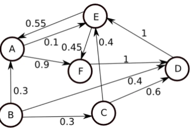
2.1 A weighted directed graph . . . 19
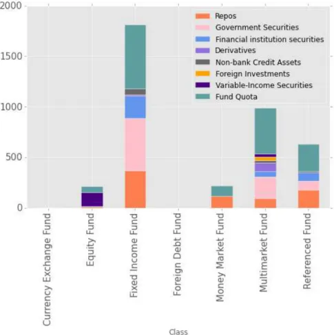
2.2 Portfolio composition by fund class. Fixed income funds represent most
of the total asset in the industry. Fund quotas is by far the most owned
asset, representing a potential source of contagion. Brazilian government
bonds follow as second most owned asset. . . 31
2.3 Number of funds by fund class. Multimarket funds represent the largest
class in number of funds, followed by fixed-income and equity funds.
Funds with more risk appetite are more numerous but smaller in total
assets. . . 32
2.4 Stability of the Investment Fund network. The table shows Jaccard
coeffients of edges and nodes for the network in pairs of months over the
period from Jan/2012 to Dec/2014. . . 33
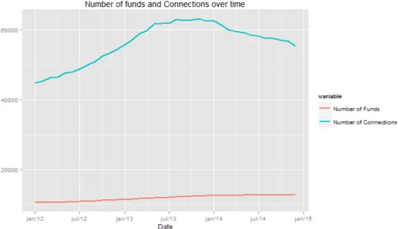
2.5 Number of nodes and connections on the network over time. The number
over funds grows slowly but steadily over time. The number of edges
2.6 The directionality of the edges indicates the investor fund as the tail
and the invested fund as the head. (a) In degree histogram for the
cross-holdings network. The histogram exhibit typical power law (b)
Out degree histogram for the cross-holdings network. The steepness of
the curve is much lower in the out-degree distribution. . . 34
2.7 Degree histograms for both types of nodes in the bipartite fund-asset
net-work. While both distributions exhibit characteristic power law shapes,
the hubs are much more prominent among assets than funds. . . 36
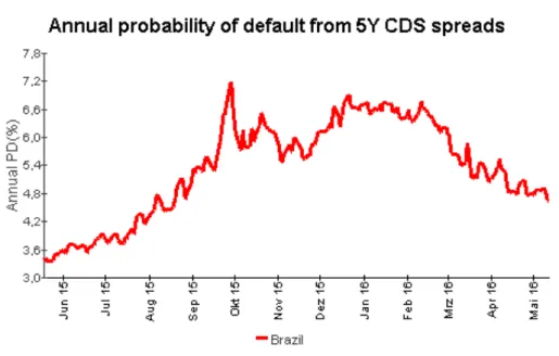
2.8 Annual probability of default from Brazilian %Year CDS spreads.. . . . 37
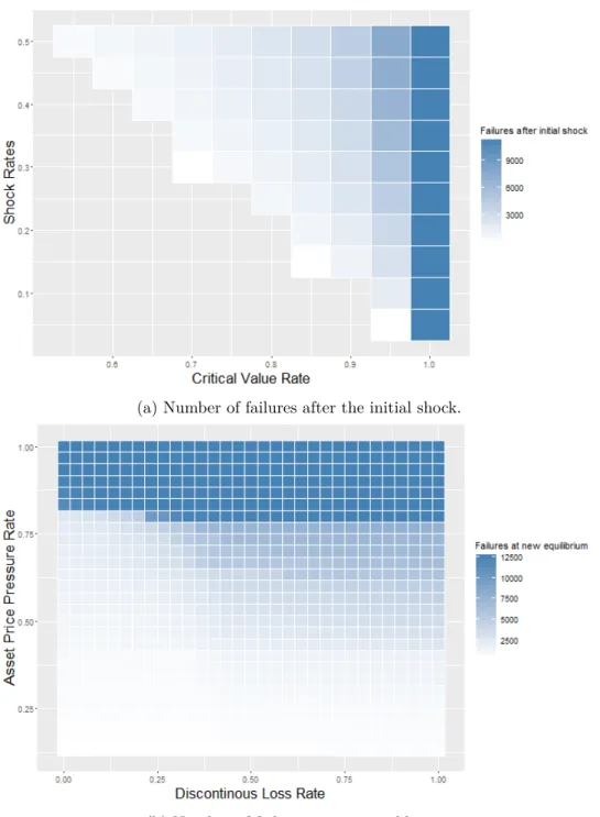
2.9 (a) Number of failures after the initial shock as we vary both the critical
value rate and the shock rate. (b) Number of final failures at a fixed
initial shock rate of 15% and critical value rate of 85% as we vary asset
price pressure rate and discontinous loss rate. . . 39
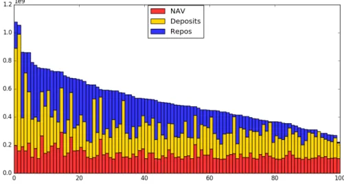
3.1 Liability composition of banks in the simulation. After initial market
creation liabilities are composed by NAV, bank deposits and repurchase
agreements. . . 64
3.2 Portfolio composition of banks in the simulation.Banks leverage to invest
in the risky asset. . . 65
3.3 Deleverage of the banking system as the the system suffers a run on the
repo. . . 66
3.4 Number of solvent, defaulted and bankrupt at each time step in our
simulation. The system reaches a new equilibrium with close to 42% of
the banks having gone bankrupt. . . 67
Lista de Tabelas
2.1 Maximum centrality observed in both networks. The Fund-Asset network
has nodes with much stronger presence as hubs. . . 35
3.1 Summary of Financial Agents. . . 64
1 Introduction 14
2 Financial Contagion in Investment Funds 15
2.1 Introduction. . . 15
2.2 Graph Theory and Network Science . . . 18
2.2.1 Graph Theory . . . 18
2.2.2 Centrality Measures . . . 20
2.2.3 Homophily and Assortativity . . . 22
2.2.4 Dynamic Networks . . . 23
2.3 The Cross-Holdings Contagion Model . . . 23
2.3.1 Primitive Assets and Cross-Holdings . . . 23
2.3.2 Firm Susceptibility to Financial Shocks . . . 25
2.3.3 The Contagion Model . . . 27
2.4 The Data . . . 29
2.5 Results and Discussion . . . 30
2.5.1 Network Topology . . . 30
2.5.2 Simulations . . . 35
2.6 Final Remarks . . . 38
13 Sumário
3 An Agent-based Model of Contagion in Financial Networks 44
3.1 Introduction. . . 44
3.2 Financial Contagion . . . 47
3.3 Agent-Based Computational Finance . . . 49
3.4 The Artificial Repo Market Model . . . 51
3.4.1 Assets . . . 51
3.4.2 Financial Agents . . . 54
3.4.3 Risk Management . . . 58
3.4.4 Market Mechanism . . . 60
3.4.5 Failures, Fire sales and Contagion . . . 61
3.5 Simulation. . . 63
3.5.1 Experimental Design . . . 63
3.5.2 Results . . . 64
3.6 Final Remarks . . . 69
Bibliography 70 A Computational Models 75 A.1 Computational Model for "Financial Contagion in Investment Funds". . 75
A.1.1 Dependencies . . . 75
A.1.2 Data . . . 76
A.1.3 Code Description . . . 77
A.2 Computational Model for "An Agent-based Model of Contagion in Fi-nancial Networks" . . . 78
A.2.1 Dependencies . . . 78
A.2.2 Object-Oriented Model . . . 78
Introduction
This dissertation explores the modeling of financial contagion and is composed by two
essays. Each study focus on different types of financial intermediaries and in different
forms interconnectivity and propagation chanels. They also propose different models
to simulate the propagation of economic shocks.
The first article, "Financial Contagion in Investment Funds", develops a cascading
failures algorithm to assess the vulnerability of investment funds to an economic shock
over the financial system. The study considers both the network of cross-holdings of
quotas and the network between assets and investment funds as connectivity measures.
Through these complementary transmition channels shocks can propagate and become
systemic. We also use data from the Brazilian Asset management to provide a
des-cription of the structure of a network of investment funds, to illustrate the proposed
algorithm and to analyse how the network structure affect the results of the algorithm.
The second article, "An Agent-based Model of Contagion in Financial Networks",
develops an artificial financial market model that simulates trading behavior in the
repo markets after a shock hits the financial system. The model is capable of simulating
a "run on the repo"with effects similar to the observed in the repo market during the
Capítulo 2
Financial Contagion in
Investment Funds
Abstract
Many new models for measuring financial contagion have been presented recently.
While these models have not been specified for investment funds directly, there are
many similarities that could be explored to extend the models. In this work we explore
ideas developed about financial contagion to create a network of investment funds using
both cross-holding of quotas and a bipartite network of funds and assets. Using data
from the Brazilian asset management market we analyse not only the contagion pattern
but also the structure of this network and how this model can be used to assess the
stability of the market.
2.1
Introduction
In recent years the use of network representations for the study of economic systems has
and production chains Allen and Babus (2008). A special subject in these topics is
the study of financial systems. Since the global financial crisis that hit the world in
2007-08 the interest in the intricate ways in which financial institutions are intertwined
has soared, with studies showing the several facets of the interconnections of financial
systems, specially in the way these connections affect global stability.
The 2007-08 crisis, which started in the US sub-prime mortgage market, rapidly
spilled over to debt markets in a process of financial contagion that ultimately led to
the demise of major American and European banks and triggered a world recession that
spanned years. Interconnection is also a cause of major concern in the ongoing European
debt crisis, with worries that the interconnection in the European bank system may
cause a serious crisis if one nation defaults on its sovereign debt or enters into recession
putting some of the external private debt at risk.
Due to the aforementioned events, much of the studies on the connectedness of
financial institutions is focused on the mutual exposures between banks, specially the
ones acquired on the interbank market (see Cocco et al. (2009),Mistrulli (2011) and
Iori et al. (2006)). But more recently some attention has been devoted to non-bank
financial intermediaries, such as the studies being conducted by the Financial Stability
Board to address what in being called the "Shadow Banking System" (Board (2011a)
and Board(2011b)). In this work, we aim to explore one of these elements of financial
systems, the asset management industry.
In the Brazilian market, in 2014, asset management firms oversaw the allocation
of approximately U$ 1T in financial assets, consisting of a substantial part of the
Brazilian financial system. Not only is the industry significant in size, but these firms
and the funds they manage transact with other institutions in the financial system,
and within themselves, in a variety of ways. As a consequence, this industry is heavily
interconnected with the bank and insurance markets, augmenting greatly the effects it
17 2.1. Introduction
While it is still highly debatable whether asset management in fact poses systemic
risk, the industry has a number of factors that make it susceptible to financial shocks.
Behaviors such as reaching for yield and herding, redemption risks associated to liquidity
mismatch, high leverage and even behaviors of the asset managers can represent sources
of risk (for a deeper discussion of the risks of asset management see the recent report
of the Office of Financial Research, U.S. Department of the Treasury(2013)). These
are factors that have the potential to amplify financial shocks over the funds and, if
the system is heavily interconnected, cause cascading failures and heavy losses to the
entire financial system.
In this paper we develop a network model to assess the inter-connectivity and
how cascading failures can occur among investment funds. We also take a empirical
approach to study the asset management market through simulations with data from
the Brazilian Market.
In a simple definition, networks can be described as collections of objects in which
some objects can be connected forming a set of links. By this generic definition, many
types of connections can be used to compose the edgeŠs set (Easley and Kleinberg
(2010)).
The literature on financial networks contains many proposed metrics which can
be used to define the connections between firms. For instance, Huang et al. (2013)
propose the use of a bipartite network between firms and assets where a link represents
a ownership relation between firm and asset, Diebold and Yılmaz (2014) propose
connectedness measures built from pieces of variance decompositions and Billio et al.
(2012) proposes a set of econometric measures based on principal-components analysis
and Granger-causality networks. In this regards we follow closely the approach adopted
by Elliott et al.(2014), in which cross-holdings of organizations shares form the edges,
taken together with the approach fromHuang et al.(2013), to better explain the effects
By forming networks considering cross-holdings and common asset holdings we can
analyze the structure of an investment fund network and look for potential impacts of
financial shocks using contagion and diffusion models. While our model uses the ideas
from the aforementioned works, this approach is not exhaustive, there are many other
contagion and diffusion models in the finance literature which could have been explored
(see Gai and Kapadia(2010) and Allen and Gale(2000)).
The structure of this paper is organized as follows. In Section 2 we provide a
background and basic terminology on graphs and networks that will be used throughout
the analysis. In Section 3 we present the contagion model using the frameworks
developed by Elliott et al. (2014) and Huang et al. (2013). Section 4 describes the
data used and give a brief overview of asset management in Brazil. Section 5 presents
the findings about the network structure and the results of simulations over the data.
Finally, in Section 6 we discuss future research directions and present a summary and
final remarks on the work.
2.2
Graph Theory and Network Science
In this section we provide some basic terminology about the concepts used along this
paper. Its comprises concepts from graph theory for the representation of networks
and from Social / Economic Network Analysis for understanding network structure and
stability.
2.2.1 Graph Theory
A graph is a mathematical construct of a set of objects, called nodes or vertices,
con-nected by a set of links, called edges. More formally a graph�= (�,�)is an ordered pair consisting of a set of nodes� and a set of edges� where� ⊆� ×�. The order of
19 2.2. Graph Theory and Network Science
Figure 2.1: A weighted directed graph
A graph may be directed or undirected. A directed graph (or digraph) is a ordered
pair �= (�,�)consisting of a set of nodes� and a set of edges� where �⊆� ×�
and where, for every edge (�,�)∈�, there is a link that leaves uand enters v. We say
that u is the tail andv is the head.
An import metric of networks is their degree distribution. The degree of a node�i
is the number of connections it has. For a digraph we define in-degree as the number
of connections incoming to a node and the out-degree as the number of connections
leaving the node.
Graph labeling is the assignment of labels to edges and/or nodes of a graph. These
labels often represent attributes of the graph. In a labeled graph we define the set of
edges� ⊆� ×�×� where� is the set of labels. Aweighted graph is a labeled graph
where edge labels are members of an ordered set, usually of integers or real numbers,
which represent the "strength" of the connections. We define�ij as the weigh between
nodes�and �.
There are many ways to represent graphs. In this work, they are usually represented
2.2.2 Centrality Measures
Graphs are a natural way to represent networks, but social economic networks usually
exhibit some properties better analyzed through specific metrics. As was found by
Albert and Barabási (2002), many real networks exhibit a property that their degree
distributions are scale-free. In social and economic networks, this property can create a
structure where a few members of the network can gather most of the connections, thus,
controlling the flow of information in the network. This brings up the importance of
analyzing the influence of members in a network. One way to analyze this importance
is through centrality measures.
Centrality measures aim to describe how a given node relate to the network in some
aspect of its structure, such as node position in the network. Four types of centrality
measures are usually described in the network literature (Jackson et al.(2008)), each
one aiming to describe an different aspect of node importance in the network. These
are:
1. Degree Centrality: How many connections a node has;
2. Closeness Centrality: How easily a node can reach other nodes;
3. Betweenness Centrality: How central the node is in creating paths between other
nodes;
4. Eigenvector Centrality: How important (well connected) the nodeŠs neighbors
are.
Degree Centrality is considered the most classical measure of centrality and it
measures how import a node is by the number of connections it has (Freeman et al.
21 2.2. Graph Theory and Network Science
that it misses the location of the node in the network while for some applications, like
spread of processes, the position of the node in the network is a fundamental aspect.
Closeness Centralitymeasures a node importance by how close it is to any other
node in the network (Freeman et al.(1980)) . One way to measure closeness is:
�c(�) =
�−1 ︁n−1
v=1�(�,�)
, (2.1)
where�(�,�)is is the shortest-path distance between� and�, and�is the number
of nodes in the graph. In a diffusion process, the nodes with highest closeness centrality
are likely to be affect by the process more rapidly than others.
Betweenness Centrality captures how well situated a node is in terms of the
paths (Freeman et al.(1980)) in the network. The betweenness centrality of a node�is
the sum of the fraction of all-pairs shortest paths that pass through it. Mathematically
we measure betweenness as::
�b(�) = ︁
s,t∈V
à(�,�|�)
à(�,�) , (2.2)
where à(�,�|�)is the number of shortest (�,�)-paths and à(�,�)is the number of those paths passing through�. In a diffusion process, a node that has high betweenness
can control the flow of information in the network.
Eigenvector Centrality is based on the premise that a nodeŠs importance is
measured by how important its connections are (Bonacich (1972)). The eigenvector
centrality for node � is xi where � is the index of node � and xi is the principal
Ax=Úx (2.3)
where A is the adjacency matrix of the network. In diffusion process, an node
who is high on eigenvector centrality is connected to many nodes which themselves are
connected to many nodes, thus multiplying their probability of contagion.
2.2.3 Homophily and Assortativity
Social and Economic networks sometimes exhibit a property that entities are more prone
to establish connections with similar entities. This property was named homophily by
Kandel (1978). Homophily may play an important role in economic networks, since it
can mean a network can be largely segregated (Jackson et al.(2008)).
One way to measure homophily among labeled nodes is by assortativity.
Assortativ-ity measures the similarAssortativ-ity of connections in a network with relation to some attribute
or label. We define the assortativity coefficient as:
�=
︁
i�ii−︁i�i�i 1−︁
i �i�i
, (2.4)
where �ij is the fraction of edges in the network that connect a type � node to
a type � and�ij = �i�j. The matrix M is the joint probability distribution (mixing matrix) of the specified attributeNewman(2003). Assortativity may play an important
whole in financial networks as segregated financial firms may form regions of closure
23 2.3. The Cross-Holdings Contagion Model
2.2.4 Dynamic Networks
Some networks vary over time. The field that studies how networks change over time
is known as network dynamics or dynamic network analysis (DNA). The main aspects
of DNA is the analysis of the statistical properties of time varying networks and the
simulation of network changes over time. DNA is a broad field and we refer to the work
of Carley (2003) for those interested in it. For the purpose of financial networks and
contagion we focus on the stability of financial networks over time.
One way to measure network stability over time is to check the Jaccard similarity
of nodes and/or edges between pairs of successive time spans (Masys(2014)). This is
a indication of how much nodes and/or edges are formed or removed from the network
between small time steps. The Jaccard similarity coefficient is a measure of similarity
between sets. The coefficient of a set S and a set T is|�∩�|/|�∪�|, that is, the ratio
of the size of the intersection of S and T to the size of their union (Rajaraman et al.
(2012)).
2.3
The Cross-Holdings Contagion Model
In determining interconnectivity between investment funds we follow closely the model
developed by Elliott et al. (2014) for financial firms in which cross-holdings of shares
among organizations may lead to cascading failures. In the context of investment funds,
we measure cross-holdings of fundŠs quotas. We differ from the model when common
assets holdings are considered in the process and in this regard we use the framework
developed by Huang et al.(2013).
2.3.1 Primitive Assets and Cross-Holdings
In the original model developed byElliott et al.(2014) the value of organizations are
the shares of the other organizations which they hold. There are�organizations making
up a set � = 1, 2, ...,�. There is also a group of assets in the economy that may be
owned by firms and these assets compose another set� = 1,2,...,�. For investment
funds as organizations, the primitive assets are formed by assets not issued by other
investment funds and legally permitted to be bought by funds, these may be shares
of companies, corporate bonds, government bonds, derivatives, among others. Funds
can also hold shares of other funds, which creates the cross-holdings among
organiza-tions. As the funds are the only organizations in our system we shall use the terms
interchangeably from this point.
The base value of a fund is determined by the value of itŠs assets. The value of an
asset � is denoted by �k and we call p the vector containing the values of the assets
in �. We also call D the matrix which entry �ik is the share of the value of asset
� held by organization �. Complementary to D we have the matrix C in which, for
each,�,� ∈�,�ij ≥0 is the fraction of organization �owned by organization �. The
matrix C can be seen as a network of direct links between the organizations. There
is also the share �ˆii := 1−︁
i∈N�ij of organization i which is not owned by other organizations in the system. This forms the matrixCˆ.
To determine the fair value of organizations, Elliott et al.(2014) used a framework
developed byFedenia et al.(1994) andBrioschi et al.(1989). The value�iof organization
� is determined by the value of itŠs assets plus the value of itŠs applications on other
organizations:
�i = ︁
k
�ik�k+ ︁
j
�ij�j (2.5)
25 2.3. The Cross-Holdings Contagion Model
V= (I−C)−1Dp (2.6)
Brioschi et al. (1989) and Fedenia et al. (1994) argue that the true value of an
organization is better captured by what is held byoutsideinvestors. This value is equal to�˙i =�ˆii�i, leading to:
˙
V=Cˆ(I−C)−1Dp=ADp (2.7)
We also callA =Cˆ(I−C)−1 the dependency matrix. It captures the true value
of the cross-holdings of quotas in the market and allow us to measure the true value of
the funds and how changes in one organizationŠs value shall affect any other.
2.3.2 Firm Susceptibility to Financial Shocks
Organizations can lose value in discontinuous ways under certain situations. We call
these losses failure costs. Failure costs are assumed if an organization falls bellow some
value threshold, in which case we can interpret that it has transitioned from a financially
stable situation to an unstable one (Elliott et al.(2014)). So, if organization �valueŠs
fall below some threshold �¯i, it incurs in failure costs Ñi(p).
In a more general setting there are many possible explanations for failure costs.
The main assumption in investment funds is that under certain situations there main
occur a run on the fund, forcing it to sell assets at inopportune times at a discount
rate, leading to the discontinuous losses. There may be many situations causing this
run on the fund, such as reputation risk generated by the asset manager, performance
risk caused by risky strategies and leverage, or economic risks such as financial bubbles
When funds are directly connected by cross holdings the spread of a discontinuous
loss is straightforward. Nevertheless, failure costs incurred by one organization may
"affect" other organizations even if they are not directly connected in the network. The
main way in which it can happen is common asset holdings. Since many assets are held
simultaneously by many firms, the way one firm incurs in failure costs can force it to fire
sale itŠs assets and force the price of the asset down in a way that other organizations
holding the same assets may also face difficulties.
To correctly address the effect of common asset holdings we use the framework
developed byHuang et al.(2013). In addition to the network of cross-holdings described
in Equation2.6we use a ancillary network formed by organizations as one type of node
and assets as the other.
In this network a link between a fund and an asset exists if the fund has the asset on
its portfolio. It is a bipartite weighted graph where the weights on the links represent
the gross value of the portfolio position in the asset.
Let B be the bipartite network between the organizations in Nand the assets in
M. We have that
B=
︀
︀ ︀
0n,n W
WT 0m ,m
︀
⎥ ︀,
where W is a�� sub-matrix where�ij is the value of the position of fund�in asset
�. We can rewrite the termDpin2.7in terms ofW. Let⃗1= [1, 1, 1,..., 1]T
n. We write:
Dp=W⃗1.
And Eq. 2.6leading to:
27 2.3. The Cross-Holdings Contagion Model
In the presence of financial instability for an organization�, not only failure costs Ñi
are incurred but also every asset� owned by� suffer a pressure to go down, becoming:
�j = ︁
i�ij−æ�ik ︁
i�ij .
2.3.3 The Contagion Model
Financial contagion can occur when one organization fails and itŠs losses spread to other
organizations causing them to fail as well. This can have the potential to generate a
cascade of failures, potentially breaking the financial system as a whole.
The financial contagion process can be described as a diffusion process where losses
spread in the network of interconnections. Through both the cross-holdings connections
and common asset holdings funds can be affected by this diffusion process.
If funds are directly connected, discontinuities will propagate in the cross-holdings
network, affecting the final value of other funds invested in the broken firms in the path
of connections. These affected funds, in turn, may start to face difficulties and cause
new failures and discontinuous losses. At the same time, these funds may be forced to
sell their assets, causing drops in asset prices which may also cause new failures and
discontinuous losses. These losses shall propagate until a new equilibrium is reached.
But prior to contagion we must have a shock over the system. This shock can be of
any kind, but for the contagion to be triggered at least one fund must lose value until
it fall bellow the critical value to move the system from equilibrium.
Bellow we describe an algorithm containing the step-by-step process to simulate
the cascading failure process.
1. Let�tbe the set of failed organizations at step�. We initialize�0 =∅, indicating
a starting state of equilibrium.
2. At the initial moment we shock a market asset �i or a set of assets M =
the nature of the shock). Each asset is reduced to a fraction of its original value
Ö�i, whereÖ <1 is determined by the strength of the shock.
3. After the initial shock, the loss spreads in the network of cross-holdings and we
recalculate the value of each fund in the system using Equation2.8, checking which
of them have fallen bellow a critical value�crit. Each fund �in which �i < �crit(i)
is added to �.
4. We start the iterative process. At step t, Let ˜bt−1 be a vector with element ˜
bi = Ñi if�∈�t−1 and 0 otherwise, whereÑi is the loss in value due to failure. Also, for each asset �j connected with each fund � in �t−1, its overall market
value is reduced as the marketŠs reaction to the fund failure. The price of asset�j
owned by �becomes �i = ︁
i�ij−æ�ij ︁
i�ij
, where æ is a parameter that measures
the strength of the fire sales over the market price of the asset .
5. The new set �t is formed by the funds which have negative values in:
A︁W⃗1−˜bt−1︁
−vcrit.
6. We terminate if �t=�t−1. Otherwise, we go back to step 4.
This algorithm provides a framework to understand how damages spread to both
other funds and to assets until the cascading failure stops. It also describes a hierarchy
of vulnerability under a specific crisis which is determined by the initial shock.
Many parameters can affect the results of the algorithm. The strength of the initial
shock, the assets affected by the shock, the critical value of the funds, the strength of
the discontinuous losses and of the fire sales are all inputs of the algorithm and must
be determined ex-ante.
Next we will present data taken from the Brazilian asset management industry and
29 2.4. The Data
2.4
The Data
Investment funds , sometimes referred to as collective investment vehicles, are financial
intermediaries that collect financial resources from a pool of investors, both individuals
and companies, and apply these resources into a pool of assets (Bodie et al.(2009)).
In Brazil, investment funds are regulated by the Securities and Exchange Comission
of Brazil (CVM) through CVM Instruction 555 (ICVM 555)1 2. Investment funds are
devoid from legal personality, despite that, they are capable of acquiring and transferring
assets and rights, always represented by their administrators and managers (Fortuna
(2008)).
Traditionally, funds are classified as fixed income and variable income to discriminate
the level of risk of their strategies. Fixed income funds invest in assets with a fixed
return rate, such as government bonds and private credit, and variable income funds
investing in assets with returns that vary with the market, such as shares of companies.
This classification can be refined to better represent investment strategies, two common
classifications are provided by the Brazilian Financial and Capital Markets Association
(Anbima) and by CVM. In this work we will adopt the classification used by CVM.
According to CVMŠs classification, funds are organized in 7 classes which reflect their
investment strategies and profile of risk according to the assets they can buy.
Fixed-income funds are the most representative class in terms of total assets and Multimarket
funds comprise the class with biggest number of funds. Multimarket funds are the class
with most diverse strategies and portfolios, as can be seen in figure2.2.
Another broadly used classification is for open-ended, which are funds open to
redemption at any time after a determined grace period, and closed-ended funds, for
1
ICVM 555 is the current legal diploma for the regulation of investment funds, but many of the classifications used in this paper are based on the definitions of CVM Instruction 409, which was the legal diploma in the period of the analysis.
2
funds with strict restrictions or even completely unavailable for redemption. 3.
Open-ended funds are the majority both in number of funds and in number of assets under
management. Close-ended funds are excluded in simulations, since they are much less
susceptible to events that could trigger failure costs, as modeled in this work, such as
a run on the fund.
For this study we used data of investment funds from the CVM database. To analyze
the network structure we used data from January 2012 up to December 2014 and for
the simulations we used data from December 2014.
2.5
Results and Discussion
2.5.1 Network Topology
To better understand how the market is organized we take a brief look at some key
fea-tures of the network topology. We then proceed to present the results of the simulation
experiments and discuss the role of the topology in the systemŠs dynamics.
Stability
The structure of the network and itŠs stability over time reflect investment decisions
from asset managers. As in Masys (2014) Jaccard similarity coefficients are used to
measure the structural stability of the network over pairs of successive periods. Figure
2.5shows the network growth over time and Figure2.4reports a summary of the Jaccard
coefficients. The network exhibit considerable stability between successive months, the
number of nodes exhibit growth at a steady rate while the number of connections seems
to fluctuate more, exhibiting a hump. This fluctuation may indicate some relationship
between the edge count and economic variables which could be further investigated.
3
31 2.5. Results and Discussion
33 2.5. Results and Discussion
Figure 2.4: Stability of the Investment Fund network. The table shows Jaccard coeffients of edges and nodes for the network in pairs of months over the period from Jan/2012 to Dec/2014.
On average, more then 90% of connections are stable between periods, which support
running dynamic models (Snijders et al.(2010)) such as the cascading failures model.
Network Metrics
The cross-holdings network has very low connectivity with an average degree of�avg=
4.34. The degree histogram shows a typical scale free distribution but in-degree and
out-degree curves have very different shapes as can be seen in Figure2.6. The highest
in-degree is 889 and highest out-degree is 70. The in-degree is the most interesting
metric since it is the one that shows how many other funds are directly affected by the
spreading of losses in the cross-holdings network.
The fund-asset network, on the order hand, has an average degree of �avg=20.23.
If we disregard cash, which is connected to almost all funds, the highest asset in-degree
of 4838. The degree distribution in Figure 2.7 shows that a few assets are present in
Figure 2.5: Number of nodes and connections on the network over time. The number over funds grows slowly but steadily over time. The number of edges fluctuates.
(a) In degree histogram (b) Out degree histogram
35 2.5. Results and Discussion
Comparing the two networks we can observe that the fund-asset network is much
more dense, with values of 0.001070 for the fund-asset network and 0.00034 for the
cross-holdings network. In Table 3.1 we can see that in the fund-asset network there
are some very central nodes while in the cross-holding network this metric is much
weaker. While assortativity is not a relevant metric in the fund-asset network, in the
cross-holding network we can observe some level of segregation. Most notably, funds
from same Administrators show assortativity of 0.502 and funds from the same class
exhibit assortativity of 0.217. While the segregation of funds of the same class is not
high enough to indicate regions of confinement for the spread of risk, the segregation
among administrators may be an issue of attention.
Table 2.1: Maximum centrality observed in both networks. The Fund-Asset network has nodes with much stronger presence as hubs.
Cross-Holdings Network Fund-Asset Network
Max. Degree Centrality 0.069 0.256
Max. Closeness Centrality 0.006 0.437
Max. Betweenness Centrality 5.98e-05 0.035 Max. Eigenvector Centrality 0.788 0.670
The nature of the spreading process in this model is very different in the cross-holding
network and in the bipartite network of funds and assets. The results above indicate
that we could observe a faster spreading of contagion caused by asset connections than
by cross-holding connections, this is due to the fact that the network is more dense and
central assets play a stronger whole as hubs.
2.5.2 Simulations
In this section we illustrate how the use of some network metrics combined with the
contagion model can be used to monitor the stability of the financial system and to
identify institutions and assets that could rapidly trigger a contagion process. We build
(a) Degree histogram for fund nodes. (b) Degree histogram for asset nodes.
Figure 2.7: Degree histograms for both types of nodes in the bipartite fund-asset network. While both distributions exhibit characteristic power law shapes, the hubs are much more prominent among assets than funds.
we can see in Figure 2.8, stressing the system to a sovereign debt default.
Sovereign debt default can occur in many forms. A sovereign debt is a contractual
obligation and the most clear-cut example of default is the failure to meet these
obliga-tions to pay interest or principal on the due date. Another example is the failure by
the government to honor debt it has guaranteed where there are clear provisions for
the guarantor to make timely payment.
But sovereign defaults are often not so explicit. Government responses to financial
distress can take many forms. In some cases, it can be inferred that, even in the absence
of an interruption of debt payments, a default has occurred because actions by the
government result in economic losses by creditors,which can vary widely (Beers et al.
(2014)).
In our network of funds and assets Federal Government Bonds occupy a very central
position. It has a total market cap of 35.12% of the total assets and it also has a degree
centrality of 4838, the biggest among all assets except for Cash. ItŠs average path length
2.19, showing that losses can affect almost any other asset price in the first time step
of the algorithm.
37 2.5. Results and Discussion
Figure 2.8: Annual probability of default from Brazilian %Year CDS spreads.
test the susceptibility of the network in diverse settings. The most important parameters
are the rate of discontinuous loss suffered by funds whenever they fail, the asset prices
factor æ, which affects assets of failed funds, the critical value under which the funds
will fail and the size of the initial shock.Three results are evaluated: the number of
firms failed by the financial shock, the number of total failures caused by the cascading
process and the number of iterations before the system reaches a new equilibrium.
Figure2.9a shows the number of initial failures caused by the initial shock as we
vary the size of the shock and the critical value of organizations. The number of failures
is small when the values are close but escalates quickly as the shock becomes much
stronger than what investors would tolerate. Figure 2.9b shows the number of final
failures as we vary the discontinuous loss rate and the asset pressure rate at a fixed
initial shock rate of 30% and critical value rate of 70%. The asset pressure rate have
a much bigger effect on the number of failures , at a rate of 30% it leads to a total
meltdown of the system independently of the discontinuous loss rate. The discontinuous
These results support our initial hypothesis that the asset network could have a
much bigger influence in the final outcome of the contagion due to the network structure
and the nature of hubs. We emphasize that we do not see these results as robust, but
merely as illustrative of the dynamic of the process.
2.6
Final Remarks
Financial contagion is a complex phenomena with possibly devastating consequences
to financial systems. Here, extending on previous work from Elliott et al. (2014) and
Huang et al.(2013), we have developed a model that accounts for both cross-holdings
among organizations and pressure over asset prices using two complementary networks.
The approach we have developed can be a valuable tool for financial supervisors
and asset managers. For instance, the algorithm can be used with scenario testing to
understand the impact of possible financial crisis to guide supervision and investment
decisions. And, while we do not know if the topological assumptions of the model hold
for other financial firms, we do believe the framework is still valuable for the study
of contagion processes over other financial intermediaries such as banks and insurance
companies.
Although we believe these results are of great value for building a theoretical
un-derstanding of financial contagion, the results obtained in this model would hardly be
reproducible in a real economy since it doesnŠt consider interaction with other financial
intermediaries, existing regulatory measures and the direct intervention of financial
regulators and/or government bailout.
Several improvements to the modeling process are possible to make it more realistic
and closer to the observable reality. To advance this line of research: (1) More work is
required to understand critical values under which discontinuities occur and the value
39 2.6. Final Remarks
(a) Number of failures after the initial shock.
(b) Number of failures at new equilibrium.
needs to be better determined, (3) a better model of financial shocks should be explored,
(4) the interaction with other financial intermediaries should be included and, (5) The
Bibliography
Albert, R. and Barabási, A.-L. (2002). Statistical mechanics of complex networks.
Reviews of modern physics, 74(1):47.
Allen, F. and Babus, A. (2008). Networks in finance.
Allen, F. and Gale, D. (2000). Financial contagion. Journal of political economy, 108(1):1Ű33.
Assaf Neto, A. (2001). Mercado financeiro.
Beers, D., Nadeau, J.-S., et al. (2014). Introducing a new database of sovereign defaults.
Technical report, Bank of Canada.
Billio, M., Getmansky, M., Lo, A. W., and Pelizzon, L. (2012). Econometric measures
of connectedness and systemic risk in the finance and insurance sectors. Journal of Financial Economics, 104(3):535Ű559.
Board, F. S. (2011a). Shadow banking: Scoping the issues. A Background Note of the Financial Stability Board (Basel.
Bonacich, P. (1972). Factoring and weighting approaches to status scores and clique
identification. Journal of Mathematical Sociology, 2(1):113Ű120.
Brioschi, F., Buzzacchi, L., and Colombo, M. G. (1989). Risk capital financing and
the separation of ownership and control in business groups. Journal of Banking & Finance, 13(4):747Ű772.
Carley, K. M. (2003). Dynamic network analysis. Citeseer.
Cocco, J. F., Gomes, F. J., and Martins, N. C. (2009). Lending relationships in the
interbank market. Journal of Financial Intermediation, 18(1):24Ű48.
Diebold, F. X. and Yılmaz, K. (2014). On the network topology of variance
decom-positions: Measuring the connectedness of financial firms. Journal of Econometrics,
182(1):119Ű134.
Easley, D. and Kleinberg, J. (2010). Networks, crowds, and markets: Reasoning about a highly connected world. Cambridge University Press.
Elliott, M., Golub, B., and Jackson, M. O. (2014). Financial networks and contagion.
Available at SSRN 2175056.
Fedenia, M., Hodder, J. E., and Triantis, A. J. (1994). Cross-holdings: estimation
issues, biases, and distortions. Review of Financial Studies, 7(1):61Ű96.
Fortuna, E. (2008). Mercado financeiro: produtos e serviços. Qualitymark Editora
Ltda.
Freeman, L. C., Roeder, D., and Mulholland, R. R. (1980). Centrality in social
networks: Ii. experimental results. Social networks, 2(2):119Ű141.
Gai, P. and Kapadia, S. (2010). Contagion in financial networks. InProceedings of the Royal Society of London A: Mathematical, Physical and Engineering Sciences,
43 Bibliography
Huang, X., Vodenska, I., Havlin, S., and Stanley, H. E. (2013). Cascading failures in
bi-partite graphs: model for systemic risk propagation. Scientific reports, 3.
Iori, G., Jafarey, S., and Padilla, F. G. (2006). Systemic risk on the interbank market.
Journal of Economic Behavior & Organization, 61(4):525Ű542.
Jackson, M. O. et al. (2008). Social and economic networks, volume 3. Princeton
University Press Princeton.
Kandel, D. B. (1978). Homophily, selection, and socialization in adolescent friendships.
American journal of Sociology, pages 427Ű436.
Masys, A. J. (2014). Networks and network analysis for defence and security. Springer
Science & Business Media.
Mistrulli, P. E. (2011). Assessing financial contagion in the interbank market:
Max-imum entropy versus observed interbank lending patterns. Journal of Banking & Finance, 35(5):1114Ű1127.
Newman, M. E. (2003). Mixing patterns in networks. Physical Review E, 67(2):026126. Office of Financial Research, U.S. Department of the Treasury (2013). Asset
manage-ment and financial stability. Technical report.
Rajaraman, A., Ullman, J. D., Ullman, J. D., and Ullman, J. D. (2012). Mining of massive datasets, volume 77. Cambridge University Press Cambridge.
Snijders, T. A., Van de Bunt, G. G., and Steglich, C. E. (2010). Introduction to
An Agent-based Model of
Contagion in Financial Networks
Abstract
This work develops an agent-based model for the study of how the leverage through
the use of repurchase agreements can function as a mechanism for the propagation
and amplification of financial shocks in a financial system. Based on the analysis of
financial intermediaries in the repo and interbank lending markets during the 2007-08
financial crisis we develop a model that can be used to simulate the dynamics of financial
contagion.
3.1
Introduction
In recent years, the use of complex models for the analysis of financial contagion in
economic systems has become widely used. The recent 2007-08 financial crisis, regularly
attributed to the complex relationships among financial institutions, has revived the
45 3.1. Introduction
interlinkages which serve as channels for the transmission and amplification of economic
shocks.
The crisis, which started with a liquidity drain in the US sub-prime mortgage
market, due to the collapse of a bubble in the housing market, quickly overflowed to
debt markets and stock markets in a process of financial contagion that eventually
prompted the downfall of major American and European banks and triggered a world
recession. The means by which the crisis spread from a specific bubble to the whole
financial system is what we call financial contagion and it is a process made possible
by the existing interconnectivity between financial institutions.
Financial institutions are interconnected in a variety of ways, both directly and
indirectly. Direct interconnectedness happen mostly through mutual credit exposures
while indirect interconnectedness occurs mainly through common asset holdings, margin
call losses and haircut increases triggered by fire sales and liquidity drain and information
spillover (Liu et al.(2015)).
Direct interconnectedness occurs because mutual credit exposures between financial
institutions can lead to domino effects. With the complex chains of intermediation which
exist in the global financial system, the failure of a highly interconnected institution can
cause major disruptions to the financial system as a whole as this institution wouldnŠt
be able to fulfill itŠs obligations and cause mark-to-market losses in the balance sheets
of all other institutions with direct exposure to it, which could cause a number of other
institutions to face distress as well.
Indirect interconnectedness occurs as institutions facing distress can start fire selling
itŠs assets. Fire sales further stress the market prices of the assets owned by the company,
causing mark-to-market losses in all institutions with common asset holdings and causing
increases in margin calls and haircuts in repurchase agreements backed by these assets.
Information spillover can also cause other institutions with similar balance sheets to
As more institutions suffer losses and become distressed, market conditions may
further deteriorate via the aforementioned contagion channels, leading to a negative
feedback loop and, possibly, to a cascade of failures.
While many approches to understand the dynamics of financial contagion using
equation-based modeling have been developed, mostly through economic and network
models (see Gai and Kapadia (2010), Huang et al. (2013) and Elliott et al. (2014)),
these approaches have the limitation of reproducing an homogenized and simplified
approximation of the observed reality, sometimes producing unrealistic models which
are not sufficiently justified (Helbing and Balietti(2010)).
In this work we focus on the prospects of the computer simulation of economic
systems to model the dynamics of financial contagion. Agent-based modeling is a
computational technique where the components of a system are encapsulated as agents,
which can represent individuals, groups, companies and/or countries, while the analysis
of the system is carried out through the interactions of these agents (Helbing(2012)).
By modeling the financial system through the use of agents, we are capable not
only of creating simulations that reflect the interactions between different entities more
accurately, but also of testing the implications of different hypothesis. We furthermore
emphasize the importance of building models using a range of empirical observations
to design more realistic models which are capable of representing market dynamics
observed in historical episodes and allows us to explore in more detail the dynamics of
financial markets.
In this work we focus on modeling one of the most prominent effects of the
2007-08 financial crisis: the liquidity drain observed in the repurchase agreement (repo)
markets. During the crisis both interbank lending and repurchase agreements shrank
dramatically, causing a massive deleverage in the financial system and threatening
several banks with insolvency in a movement that only stopped through a government
47 3.2. Financial Contagion
market funds and hedge funds in the repo and interbank markets in order to recreate
this financial contagion movement.
The remainder of this paper is structured as follows. In Section3.2 we introduce
the problem of financial contagion and focus on the repo markets. Section3.3discusses
agent-based models of financial markets and how they can be used to understand
market dynamics such as the one we wish to model. Section 3.4 presents our
agent-based financial contagion model. In Section3.5we perform some numerical simulations
and discuss the results. Finally, in Section 3.6 we discuss extensions of the proposed
method and our conclusions.
3.2
Financial Contagion
Strong financial contagion has been one of the key features of most recent financial
crises, as localized problems in certain segments of the markets spread to other segments
leading to the risk of cascading defaults and failures which are often avoided through
government bailouts of institutions deemed "too big to fail".
As described byGorton and Metrick(2009), the panic of 2007-08 occurred through
a run on the repo market. The repo market is very important market that provides
collaterized financing for banks.They work very much like bank deposits, but for firms
operating in the capital markets. In a repurchase agreement the bank sells a security
with the promise of repurchasing the security at a specified price in the end of the
contract. The intermediary buying the security from the bank is remunerated by the
spread in operation.
According toGorton and Metrick (2009), in the last twenty-five years a number of
financial innovations have allowed traditional assets of banks to be traded in capital
markets through securitization and loan sales and have allowed banks to leverage
Since the 2007-08 crisis, the interconnected nature of financial markets has not
only been studied as an explanation for the spread of risk and losses throughout the
system, but also motivated much of the policy recommendations in the aftermath. Yet,
a framework to understand how the dynamics of the network structure of the financial
market, specially the repo market, leads to systemic risk remains incomplete.
In a broader sense, there is currently a high level of uncertainty about which elements
in the structure of the financial system causes contagion and how it occurs. Early work,
prior to the crisis, focused on general aspects of interbank lending such as the work of
Allen and Gale(2000), which modeled contagion as an equilibrium phenomenon caused
by liquidity preference shocks through economic regions, and of Rochet and Tirole
(1996), which considers the systemic risk created by interbank lending and investigates
whether decentralized bank interactions can be preserved while maintaining the stability
of the system.
More recent work, such as Gai and Kapadia (2010), Acemoglu et al. (2013) and
Elliott et al.(2014) examine how shocks propagate through a network based on debt
holdings or interbank lending and, also, how shocks propagate as a function of network
architecture.
While these works have provided useful insights about financial contagion (although
presenting quite different and complementary results), the use of economic equilibrium
and network models have some limitations in the study of the phenomenon. For
instance, financial agents usually have different goals and strategies, thus, behaving
very differently. Also, we must consider that the nature of debt exposures as connectivity
measures can also vary greatly, with mutual lending exposures, cross-holding of shares,
repurchase agreements and common asset holdinds of other sorts (e.g. stocks) having
a different impact on the propagation of shocks.
Accounting for these heterogeneities in network and economic models can lead to
49 3.3. Agent-Based Computational Finance
accurate representation of the financial system, despite being unable to render an
analytical solution to understand the problem, is to use agent-based simulation, as we
describe bellow.
3.3
Agent-Based Computational Finance
Much of the work in economics and finance hopes to simplify human interactions and
behaviors in a way that we can analyze these systems through aggregated macro-features.
But complex systems involves complex interactions among many individuals and, in
some cases, this complexity makes the use of analytical models to understand the
system unfeasible. For this reason, agent-based models and simulations have become
an invaluable tool for understanding the dynamics of the economic and/or financial
system as a whole.
Agent-based models are a class of computational models used to simulate the actions
and interactions of autonomous agents (Gilbert(2008)). In computational economics,
these models have been used to study properties of markets by building and simulating
markets, especially in the field of computational finance and there are many ways in
which agent-based models can be used to study financial markets1
The building of artificial markets is one of the most important contributions of
agent-based models to the study of financial systems. They allow us to model economic agents
according to a theoretical model and to observe if our economic assumptions about the
agents interactions in a financial setting would generate the expected dynamics.
Since the eighties some models of artificial markets have been tried, specially for
stock markets. Cohen et al.(1983) tried to look the impact of random behaving agents
on various market structures, while Kim and Markowitz (1989) used discrete event
1
simulation to model the interactions of different kinds of trading agents andDe Grauwe
et al. (1995) focused on the dynamics of foreign exchange markets.
One of most notable and most sophisticated markets is the Santa Fe Institute (SFI)
market. The SFI market was created with the idea of modeling a financial market
with an ecology of trading strategies (LeBaron (2002)). The SFI Market structure
was modeled to consider preferences and risk aversion in trading and even allowed
the emergence of trading patterns over time through the use of genetic algorithms.
Although there have been several generations of the SFI artificial market, consisting
of modifications of the market structure and of different programming platforms, the
fundamentals of the theoretical model have persisted2.
Other artificial stock markets have been designed focusing on features not included
in the SFI artificial market model. For instance,LeBaron(2001b) andLeBaron (2001a)
have used a new framework including varying forecasting horizons and memory lengths,
which is crucial in the convergence to a rational expectations equilibrium, while
Ser-guieva and Wu (2007) have investigated herding behaviors as a possible reason for
contagion among different markets, and Martinez-Jaramillo and Tsang (2009) have
elaborated an artificial market in which trading behaviors model technical,
fundamen-tal and noise traders, being able to recreate statistical properties of price series in real
financial markets.
Outside of stock markets, Arciero et al.(2008) developed a model of real time gross
settlement paying system for predicting the impact of disruptive events in the flow of
interbank payments andLlacay and Peffer (2010) developed a model to simulate crisis
and risk management in fixed-income markets.
Agent-based models of financial markets have allows to simulate and recreate
episodes observed in historical data to assess economic theories. In this work we
2
51 3.4. The Artificial Repo Market Model
focus on building an artificial repo market and itŠs behavior under a liquidity shock.
3.4
The Artificial Repo Market Model
To simulate the dynamics of financial contagion in the repo market we build an artificial
financial market where financial agents must manage their risk and may face defaults
and bankruptcy if there are significant imbalances between their balance sheets. The
financial risk is measured and controlled trough losses, liquidity and leverage metrics.
Our artificial market structure is designed to reflect financial intermediaries that
may choose to invest in a set of tradeable assets from outside the financial system
(representing economic projects) and that can also make operations among themselves
to improve resource allocation.
We design three types of financial intermediaries as agents, which can be banks,
money market funds (MMFs) or hedge funds. These intermediaries interact with each
other trading assets according to their roles, as described bellow, and with an
optimiza-tion strategy. Every intermediary tries to maximize their gains while managing their
risk.
3.4.1 Assets
For the assets that can be traded by the agents, there is a risk free government bond,
a stock, representing a risky liquid asset, and a risky fixed-income asset (from this
point only called risky asset), representing a economic project financed and securitized
by banks. The intermediaries can also trade resources through interbank lending and
repurchase agreements. These serve as instruments for them to improve resource
allocation, and manage risk.
List of Assets:
In our market there is a government bond, consisting of a risk free asset, paying a
constant interest rate, �f =0.10. This asset has complete liquidity as there is we assume there are external agents willing to match the order imbalance (treasury,
foreign investors, central banks, etc.).
B) Stock
There is also a risky stock, similar to the one described inLeBaron(2002), paying
stochastic dividend following the autoregressive process:
�t=�¯+�(�t−1−�¯) +Ût (3.1)
with �¯ = 10, � = 0.95 and Û
t ∼ �(0,àµ2). The price of the stock is determined endogenously in the market.
C) Risky Asset
There is a risky asset paying a constant interest rate�r=0.11. This asset represents an economic project financed by banks and securitized in the capital markets. This
asset can lose liquidity fast and may be a major source of risk. Since we do not
implement mark-to-market calculation of bond prices, mainly because there are
no variation in Government Bond interest rates, the higher interest rate reflects
exclusively the perceived liquidity risk and the default risk of the asset.
D) Interbank Loan
Interbank lending play a key role in the financial system. They are vital for banksŠ
liquidity management.The interbank lending market is constituted by unsecured
loans (the interbank loan) and secured loans (through repurchase agreements and
53 3.4. The Artificial Repo Market Model
The interbank loan is an operation where banks extend loans to one another for a
small term. In our model they are used when banks donŠt have access to secured
loans and must meet liquidity or cash requirements to avoid a default. The interbank
loan has an interest rater�IL = �f +Ói where Ói is the risk premium paid by the borrower and:
Ói =
︁ j��ij ︁
�i�sell(�)
(3.2)
where ��ij is the value of interbank loan issued from bank� to bank�, �i is the
total value of asset�owned by the bank�and�sell(�i)is the probability of selling the asset�at each timestep, which is determined by the liquidity index of the asset,
defined in Subsection 3.4.3. Interbank loans are always overnight.
E) Repurchase Agreement
Repos are a key mechanism in our fixed-income market. Repos require margining
practices, where the borrower pays an initial margin, or ŚhaircutŠ, to provide some
protection to the lender in case the other party defaults.
In our market, we implement a simplified version of repo operations3. Repos
can be backed up by Government Bonds or by the Risky Asset. Also, repos, as
interbank loans, are always overnight, but can be renewed at each time step. We
also implement margining pratices with the haircut being calculated as:
�������=1−�sell(�) (3.3)
3