Edges, Chains, Shadows, Neighbors and
Subgraphs in the Intrinsic Order Graph
Luis Gonz´alez
Abstract—Many different scientific, technical or social phe-nomena can be modeled by a complex system depending on a large numbern of random Boolean variables. Such systems are called complex stochastic Boolean systems (CSBSs). The most useful representation of a CSBS is the intrinsic order graph. This is a symmetric digraph on 2n
nodes, with a char-acteristic fractal structure. In this paper, different properties of the intrinsic order graph are studied, namely those dealing with its edges; chains; shadows, neighbors and degrees of its vertices; and some relevant subgraphs, as well as the natural isomorphisms between them.
Index Terms—complex stochastic Boolean system, edges, intrinsic order graph, neighbors, shadows, subgraphs.
I. INTRODUCTION
I
N this paper, we consider complex systems depending on an arbitrary number n of random Boolean variables x1, . . . , xn, the so-calledcomplex stochastic Boolean systems(CSBSs). That is, the n system basic components xi are assumed to be stochastic (i.e., non-deterministic), and they only take two possible values: 0, 1.
So, each one of the2n possible situations (outcomes) for a CSBS is given by a binary n-tuple u = (u1, . . . , un) ∈
{0,1}nof 0s and 1s, and it has its own occurrence probability
Pr{(u1, . . . , un)} [11]. Throughout this paper, the n basic components of the system are assumed to be statistically independent.
Using the classical terminology in Statistics, a stochas-tic Boolean system can be modeled by the n-dimensional Bernoulli distribution X = (x1, . . . , xn)with sample space
{0,1}n, and parametersp1, . . . , pn defined by
Pr{xi = 1}=pi, Pr{xi= 0}= 1−pi,
so that, taking into account the statistical independence of the Bernoulli marginal variables xi, for allu∈ {0,1}n, we have
Pr{u}=
n
Y
i=1
Pr{xi=ui}= n
Y
i=1 pui
i (1−pi)1−ui, (1) that is, Pr{u}is the product of factorspi ifui= 1,1−pi if ui= 0.
Example 1.1: Let n = 4 and u= (1,0,1,0) ∈ {0,1}4. Letp1= 0.1,p2= 0.2,p3= 0.3,p4= 0.4. Then using (1),
we have
Pr{(1,0,1,0)}=p1(1−p2)p3(1−p4) = 0.0144. Manuscript received October 24, 2011. This work was supported in part by the Spanish Government, “Ministerio de Ciencia e Innovaci´on”, “Secretar´ıa de Estado de Universidades e Investigaci´on”, and FEDER, through Grant contracts: CGL2008-06003-C03-01/CLI and UNLP08-3E-010.
L. Gonz´alez is with the Research Institute SIANI & Department of Mathematics, University of Las Palmas de Gran Canaria, 35017 Las Palmas de Gran Canaria, Spain (e-mail: [email protected]).
The behavior of a CSBS is determined by the ordering between the current values of the 2n associated binary n -tuple probabilities Pr{u}. Computing all these 2n proba-bilities –by using (1)– and ordering them in decreasing or increasing order of their values is only possible in practice for small values of the numbernof basic variables. However, for large values ofn, to overcome the exponential nature of this problem, we need alternative procedures for comparing the binary string probabilities. For this purpose, in [2] we have defined a partial order relation on the set{0,1}n of all the2n binaryn-tuples, the so-calledintrinsic order between binaryn-tuples.
The intrinsic order relation is characterized by a simple positional criterion, the so-called intrinsic order criterion
(IOC). IOC enables one to compare (to order) two given binaryn-tuple probabilitiesPr{u},Pr{v}, without comput-ing them, simply lookcomput-ing at the positions of the0s and1s in the binaryn-tuplesu, v.
More precisely, for those pairs (u, v) of binary n-tuples comparable by intrinsic order, the ordering between their occurrence probabilities is always the same for all sets of basic probabilities{pi}
n
i=1. On the contrary, for those pairs (u, v)of binaryn-tuples incomparable by intrinsic order, the ordering between their occurrence probabilities depends on the current values the set of basic probabilities{pi}
n i=1.
The most useful graphical representation of a CSBS is the intrinsic order graph. This is a symmetric, self-dual diagram on 2n nodes (denoted by In) that displays all the binary n-tuples from top to bottom in decreasing order of their occurrence probabilities. Formally, In is the Hasse diagram of the intrinsic partial order relation on{0,1}n.
In this context, the main goal of this paper is to present some new properties of the intrinsic order graph. In particu-lar, we give the set and the number of edges ofIn, the set and the number of elements which are neighbors (adjacent) in the graph to a fixed binaryn-tupleu∈ {0,1}n. To determine the set of neighbors of a given binaryn-tupleu, we first study its lower and upper shadows. Moreover, we also analyze some chains and subgraphs of the the intrinsic order graph. Some of these properties can be found in [9], but this paper also presents some other new properties ofIn, not described in that paper.
II. THEINTRINSICORDER
Throughout this paper, we indistinctly denote the n-tuple u ∈ {0,1}n by its binary representation (u1, . . . , un) or by its decimal representation, and we use the symbol “≡” to indicate the conversion between these two numbering systems. The decimal numbering and the Hamming weight (i.e., the number of1-bits) ofuwill be respectively denoted by
u≡u(10 =
n
X
i=1 2n−iu
i, wH(u) = n
X
i=1 ui.
Example 2.1: Letn= 6 andu= (1,0,1,0,1,1). Then
u= (1,0,1,0,1,1)≡20+ 21+ 23+ 25= 43, wH(u) = 4.
Given two binaryn-tuplesu, v∈ {0,1}n, the ordering be-tween their occurrence probabilitiesPr (u),Pr (v)obviously depends on the Bernoulli parameters pi, as the following simple example shows.
Example 2.2: Letn= 3,u= (0,1,1)andv= (1,0,0). Forp1= 0.1, p2= 0.2, p3= 0.3, using (1), we have:
Pr{(0,1,1)}= 0.054<Pr{(1,0,0)}= 0.056, for p1= 0.2, p2= 0.3, p3= 0.4, using (1), we have:
Pr{(0,1,1)}= 0.096>Pr{(1,0,0)}= 0.084. However, as mentioned in Section I, in [2] we have es-tablished an intrinsic, positional criterion to compare the occurrence probabilities of two given binaryn-tuples without computing them. This criterion is presented in detail in Section II-A, while its graphical representation is shown in Section II-B.
A. The Intrinsic Order Relation
Theorem 2.1 (The intrinsic order theorem): Let n ≥ 1. Let x1, . . . , xn be n mutually independent Bernoulli vari-ables whose parameterspi= Pr{xi= 1}satisfy
0< p1≤p2≤ · · · ≤pn≤0.5. (2) Then the occurrence probability of the binaryn-tuplev, i.e., v= (v1, . . . , vn)∈ {0,1}
n
, isintrinsicallyless than or equal to the occurrence probability of the binary n-tuple u, i.e., u = (u1, . . . , un) ∈ {0,1}
n
, (that is, for all set {pi} n i=1
satisfying (2))if and only if the matrix
Mu v :=
u1 . . . un v1 . . . vn
either has no 10 columns, or for each 10 column in Mu
v there exists (at least)one corresponding preceding
0 1
column(IOC).
Remark 2.1: In the following, we assume that the pa-rameters pi always satisfy condition (2). Fortunately, this hypothesis is not restrictive for practical applications.
Remark 2.2: The 01
column preceding each 10
column is not required to be necessarily placed at the immediately previous position, but just at previous position.
Remark 2.3: The term corresponding, used in Theorem 2.1, has the following meaning: For each two 10
columns in matrix Mu
v, there must exist (at least) two different
0 1
columns preceding each other. In other words, for each 10
column in matrixMu
v the number of preceding
0 1
columns must be strictly greater than the number of preceding 10 columns.
Claim 2.1: IOC can be equivalently reformulated in the following way, involving only the 1-bits of u and v (with no need to use their0-bits). MatrixMu
v satisfies IOC if and only if either uhas no 1-bits (i.e.,uis the zeron-tuple) or for each 1-bit in uthere exists (at least) one corresponding
1-bit in v placed at the same or at a previous position. In other words, eitheruhas no1-bits or for each1-bit inu, say ui= 1, the number of1-bits in (v1, . . . , vi)must be greater than or equal to the number of1-bits in (u1, . . . , ui).
The matrix condition IOC, stated by Theorem 2.1 or by Claim 2.1, is called the intrinsic order criterion, because it is independent of the basic probabilities pi and it only depends on the relative positions of the 0s and 1s in the binary strings u and v. Theorem 2.1 naturally leads to the following partial order relation on the set {0,1}n [2], [3]. The so-called intrinsic order will be denoted by “”, and whenvuwe say thatvis intrinsically less than or equal tou(or uis intrinsically greater than or equal tov).
Definition 2.1: For allu, v∈ {0,1}n
vu iff Pr{v} ≤Pr{u} for all set {pi} n
i=1 s.t.(2)
iff matrix Mu
v satisfies IOC.
In the following, the partially ordered set (poset, for short) fornvariables({0,1}n,)will be denoted byIn; see [12] for more details about posets.
Example 2.3: Forn= 3:
3≡(0,1,1)(1,0,0)≡4 & (1,0,0)(0,1,1) since
1 0 0
0 1 1
and
0 1 1
1 0 0
do not satisfy IOC (Remark 2.3). Therefore, (0,1,1) and
(1,0,0)are incomparable by intrinsic order, i.e., the ordering between Pr{(0,1,1)} and Pr{(1,0,0)} depends on the basic probabilitiespi, as Example 2.2 has shown.
Example 2.4: Forn= 4:
12≡(1,1,0,0)(0,1,0,1)≡5since
0 1 0 1
1 1 0 0
satisfies IOC (Remark 2.2). For all0< p1≤ · · · ≤p4≤12 Pr{(1,1,0,0)} ≤Pr{(0,1,0,1)}.
Example 2.5: For alln≥1, the binaryn-tuples
0,. . .,⌣n 0≡0 and 1,. . .,⌣n 1≡2n−1
are the maximum and minimum elements, respectively, in the posetIn. Indeed, both matrices
0 . . . 0 u1 . . . un
and
u1 . . . un
1 . . . 1
satisfy the intrinsic order criterion, since they have no 10 columns!.
Thus, for allu∈ {0,1}n and for all {pi} n
i=1 s.t. (2)
Prn1,. . .,⌣n 1o≤Pr{(u
1, . . . , un)} ≤Pr
n
Many different properties of the intrinsic order can be imme-diately derived from its simple matrix description IOC [2], [3], [5]. For instance, we have the two following necessary (but not sufficient) conditions for intrinsic order (see [3] for the proof).
Corollary 2.1: For allu, v∈ {0,1}n
uv⇒wH(u)≤wH(v), uv⇒u(10 ≤v(10. B. The Intrinsic Order Graph
In this subsection, the graphical representation of the poset In = ({0,1}
n
,) is presented. The usual representation of a poset is its Hasse diagram (see [12] for more details about these diagrams). Specifically, for our poset In, its Hasse diagram is a directed graph (digraph, for short) whose vertices are the 2n binary n-tuples of0s and1s, and whose edges go upward fromv touwheneverucoversv, denoted by u ⊲ v. This means that u is intrinsically greater than v with no other elements between them, i.e.,
u ⊲ v ⇔ u≻v and∄ w ∈ {0,1}n s.t. u≻w≻v. A simple matrix characterization of the covering relation for the intrinsic order is given in the next theorem; see [4] for the proof.
Theorem 2.2 (Covering relation inIn): Let n ≥ 1 and u, v∈ {0,1}n. Thenu⊲v if and only if the only columns
of matrix Mu
v different from
0 0
and 11are either its last column 01
or just two columns, namely one 10
column immediately preceded by one 01
column, i.e., either
Mu v =
u1 . . . un−1 0 u1 . . . un−1 1
or (3)
Mu v =
u1 . . . ui−2 0 1 ui+1 . . . un u1 . . . ui−2 1 0 ui+1 . . . un
. (4)
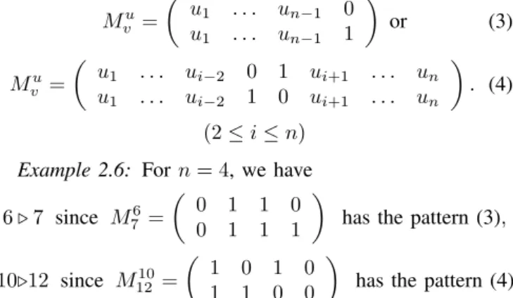
(2≤i≤n) Example 2.6: Forn= 4, we have
6⊲7 since M76=
0 1 1 0 0 1 1 1
has the pattern (3),
10⊲12 since M10 12 =
1 0 1 0
1 1 0 0
has the pattern (4).
The Hasse diagram of the posetIn will be also called the
intrinsic order graphfornvariables, denoted as well byIn. For small values ofn, the intrinsic order graphIn can be directly constructed by using either Theorem 2.1 or Theorem 2.2. For instance, forn= 1:I1= ({0,1},), and its Hasse
diagram is shown in Fig. 1.
0
|
1
Fig. 1. The intrinsic order graph forn= 1.
IndeedI1 contains a downward edge from0 to1 because
(see Theorem 2.1) 0 ≻ 1, since matrix 01
has no 10
columns! Alternatively, using Theorem 2.2, we have that
0 ⊲1, since matrix 0
1
has the pattern (3)! Moreover, this is in accordance with the obvious fact that
Pr{0}= 1−p1≥p1= Pr{1}, since p1≤1/2due to (2)!
However, for large values ofn, a more efficient method is needed. For this purpose, in [4] the following algorithm for iteratively building upIn (for all n≥2) fromI1 (depicted
in Fig. 1), has been developed.
Theorem 2.3 (Building upIn fromI1): Let n≥2. Then
the graph of the poset In ={0, . . . ,2n−1}(on 2n nodes) can be drawn simply by adding to the graph of the poset In−1 =0, . . . ,2n−1−1 (on 2n−1 nodes)its isomorphic
copy2n−1+I
n−1=2n−1, . . . ,2n−1 (on2n−1 nodes).
This addition must be performed placing the powers of2 at consecutive levels of the Hasse diagram of In. Finally, the edges connecting one vertexuofIn−1with the other vertex v of2n−1+I
n−1 are given by the set of2n−2vertex pairs
(u, v)≡ u(10,2n−2+u(10
2n−2≤u(10 ≤2n−1−1 .
Fig. 2 illustrates the above iterative process for the first few values ofn, denoting all the binaryn-tuples by their decimal equivalents. Basically, after adding to In−1 its isomorphic
copy2n−1+I
n−1, we connect one-to-one the nodes of “the
second half of the first half” to the nodes of “the first half of the second half”: A nice fractal property ofIn!
0
|
1 0
|
1
|
2
|
3 0
|
1
|
2
|
3 4
|
5
|
6
|
7 0
|
1
|
2
|
3 4
|
5 8
| |
6 9
| |
7 10
|
11 12
|
13
|
14
|
15
Fig. 2. The intrinsic order graphs forn= 1,2,3,4.
Each pair(u, v)of vertices connected inIn either by one edge or by a longer descending path fromutov, means that u is intrinsically greater than v, i.e., u ≻ v. For instance, looking at the Hasse diagram of I4, the right-most one in
Fig. 2, we observe that 5≡ (0,1,0,1) ≻12≡(1,1,0,0), in accordance with Example 2.4.
On the contrary, each pair(u, v)of non-connected vertices in In either by one edge or by a longer descending path, means thatuandv are incomparable by intrinsic order, i.e., u⊁vandv⊁u. For instance, looking at the Hasse diagram of I3, the third one from left to right in Fig. 2, we observe
that 3 ≡ (0,1,1) and 4 ≡ (1,0,0) are incomparable by intrinsic order, in accordance with Example 2.3.
Moreover, the properties of the intrinsic order stated by Example 2.5 and Corollary 2.1, are also illustrated by any of the diagrams in Fig. 2.
0 1 2 3 4
5 8
6 9 16
7 10 17
11 12 18 13 19 20
14 21 24
15 22 25
23 26 27 28
29 30 31
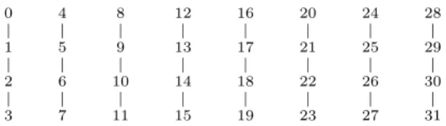
Fig. 3. The edgeless intrinsic order graph forn= 5.
For further theoretical properties and practical applications of the intrinsic order and the intrinsic order graph, we refer the reader to [5], [6], [7], [8], [9], [10].
When viewed as the natural representation of a partial order relation, the Hasse diagram of the intrinsic order is just the picture of the poset In. We refer the reader to [12], for more details about posets. When viewed as an undirected graph, the Hasse diagram is called the cover graph of the poset. We refer the reader to [1], for standard notation and terminology concerning graphs. Using Theorems 2.1, 2.2, and 2.3 we can derive many different order-theoretic and graph-theoretic properties of In. In Sections III, IV, and V, some of these properties are presented.
III. EDGES, CHAINS ANDCHAINDECOMPOSITIONS IN THEINTRINSICORDERGRAPH
A. Edges
LetVn andEn be the sets of vertices and edges, respec-tively, ofIn. As usual, |A|denotes the cardinality of the set A. As mentioned, the number of nodes of In is obviously
|Vn|=|{0,1} n
|= 2n.
Our first property gives the number of edges ofIn.
Proposition 3.1: For all n ≥ 1, the number of edges in the intrinsic order graphIn is
|En|= (n+ 1) 2n−2. (5)
Proof: The edges (going downward from uto v) in a Hasse diagram are exactly the covering relations (u ⊲ v).
Hence, using Theorem 2.2, we obtain
|En|=|{(u, v)∈Vn×Vn |u⊲v}|
=|{(u, v)∈Vn×Vn |Mvu has the pattern (3)}|+
=|{(u, v)∈Vn×Vn |Mvu has the pattern (4)}|
=
u1 . . . un−1 0 u1 . . . un−1 1
+
=
u1 . . . ui−2 0 1 ui+1 . . . un u1 . . . ui−2 1 0 ui+1 . . . un
= 2n−1+ (n−1) 2n−2= (n+ 1) 2n−2,
as was to be shown.
Remark 3.1: Using proposition 3.1, we get for alln≥2
|En|= (n+ 1) 2n−2= 2·n·2n−3+2n−2= 2|En−1|+2n−2,
a recurrence relation for the number |En| of edges of In, which could be also obtained directly from Theorem 2.2.
When we use the binary representation, the set En of all the (n+ 1) 2n−2 edges in I
n is given by Theorem 2.2.
The following proposition gives this set using the decimal numbering for the pairs of adjacent nodes (see Fig. 2).
Proposition 3.2: For alln≥1 En=
u(10, u(10+ 1
u(10 = 2p, 0≤p≤2n−1−1
[
n−2
[
m=0
u(10, u(10 + 2m
u(10 =q+ 2m(1 + 4r), 0≤q≤2m−1,
0≤r≤2(n−2)−m−1
.
Proof: The edges (going downward from u tov) in a Hasse diagram are exactly the covering relations (u ⊲ v).
So, using Theorem 2.2, we obtain
En= u(10, v(10∈Vn×Vn |u⊲v
=
u(10, v(10
∈Vn×Vn |Mvu has the pattern (3)
∪
u(10, v(10∈Vn×Vn |Mvu has the pattern (4) . On one hand, ifMu
v has the pattern (3) then we have that v(10 =u(10+ 1, and
u(10 = (u1, . . . , un−1,0)(10
= 2 (u1, . . . , un−1)(10 = 2p 0≤p≤2
n−1−1
.
On the other hand, if Mu
v has the pattern (4) then making the change of variablem=n−i, we get
v(10 =u(10+ 2n−i with2≤i≤n, i.e., v(10 =u(10 + 2m with0≤m≤n−2 and u(10 = (u1, . . . , ui−2,0,1, ui+1, . . . , un)(10
= (u1, . . . , ui−2,0,0,0, . . . ,0)(10 + (0, . . . ,0,0,1,0, . . . ,0)(10 + (0, . . . ,0,0,0, ui+1, . . . , un)(10
= 2n−i+2(u1, . . . , ui−2)(10
+ 2n−i+ (u
i+1, . . . , un)(10
= 2m+2r+ 2m+q=q+ 2m(1 + 4r),
where,0≤q≤2m−1 and0≤r≤2(n−2)−m−1.
Example 3.1: Letn= 4. Using Proposition 3.2, we get
A4=
u(10, u(10 + 1
u(10 = 2p,
0≤p≤2n
−1−1 = 7
=
(0,1),(2,3),(4,5),(6,7),
(8,9),(10,11),(12,13),(14,15)
,
B4= 2
[
m=0
u(10, u(10 + 2 m
u(10 =q+ 2 m
(1 + 4r),
0≤q≤2m
−1,
0≤r≤22−m−1
=
(1,2),(5,6),(9,10),(13,14),
(2,4),(3,5),(10,12),(11,13),
(4,8),(5,9),(6,10),(7,11)
,
where the three above rows respectively correspond to: m= 0 : q= 0 r= 0,1,2,3 v(10 =u(10+ 20 m= 1 : q= 0,1 r= 0,1 v(10 =u(10+ 21 m= 2 : q= 0,1,2,3 r= 0 v(10 =u(10+ 22
Thus, E4 = A4∪B4 contains all the 20 edges (pairs of
adjacent nodes) of the graphI4, as one can confirm looking
at the right-most diagram in Fig. 2. Note that using (5) for n= 4, we can also confirm that the cardinality of E4 is
B. Chains
Two elements u, v of a poset (P,≤) are said to be comparable if eitheru≤vorv≤u. A chain in a poset is a totally ordered subset, i.e., a subset of pairwise comparable elements. A chain u = u1 > u2 > · · · > ul = v from u to v is said to have length l −1. A chain is said to be saturated when no further elements can be interpolated between its elements. In other words, all successive relations in a saturated chain u1> u2>· · ·> ul
are coverings [12]. In particular, a saturated chain of lengthl−1 in our poset Inis a subsetu1, u2, . . . , ul of{0,1}n, such thatu1⊲u2⊲
· · ·⊲ ul, i.e., u1 ≻ u2 ≻ · · · ≻ ul with no other elements between them.
A chain decomposition of a posetP is a family of disjoint chains whose union is P. A chain cover of a poset P is a chain decomposition into saturated chains, i.e., a set of disjoint saturated chains covering the elements ofP.
Let us mention that one can define many different chain covers ofIn. The chain cover of our poset consisting of the largest possible number of chains (namely, 2n−1), with the
smallest possible length (namely,1) is stated in the following Proposition. Basically, the idea is the following: Each even number2kcovers its consecutive odd number2k+ 1.
Proposition 3.3: For all n ≥ 1 the poset In can be partitioned into the following2n−1saturated chains of length 1, that we call “congruence chains(mod 2)”:
2k ⊲2k+ 1 0≤k≤2n−1−1
.
Proof: For allk≡(u1, . . . , un−1)∈ {0,1}n−1, matrix
M2k
2k+1=
u1 . . . un−1 0 u1 . . . un−1 1
has the pattern (3). Finally, since all these chains are pairwise disjoint, and they completely coverIn, i.e.,
[
0≤k≤2n−1−1
{2k,2k+ 1}= [0,2n−1]≡ {0,1}n,
the proof is concluded.
However, the most intuitive or natural way for partitioning In into saturated chains is clearly suggested by Figs. 2 or 3. Just consider the 2n−2 “columns” obtained after n−2
successive bisections of In, containing four consecutive numbers, and beginning with a multiple 4k of 4. More precisely
Proposition 3.4: For all n ≥ 2 the poset In can be partitioned into the following2n−2saturated chains of length 3, that we call “congruence chains(mod 4)”:
4k ⊲4k+ 1⊲4k+ 2⊲4k+ 3 0≤k≤2n−2−1
. Proof: For all k ≡ (u1, . . . , un−2) ∈ {0,1}n−2, the
matrices
M4k
4k+1 =
u1 . . . un−2 0 0 u1 . . . un−2 0 1
,
M4k+1 4k+2 =
u1 . . . un−2 0 1 u1 . . . un−2 1 0
,
M44kk+3+2 =
u1 . . . un−2 1 0 u1 . . . un−2 1 1
have either the pattern (3) or the pattern (4). Finally, since all these chains are pairwise disjoint, and they completely
coverIn, i.e.,
[
0≤k≤2n−2−1
{4k,4k+ 1,4k+ 2,4k+ 3}= [0,2n−1]
≡ {0,1}n, the proof is concluded.
For instance, for n = 5 the 2n−2 = 8 “columns” or
congruence chains(mod 4)of the graphI5(depicted in Fig.
3), are shown in Fig. 4.
0
|
1
|
2
|
3 4
|
5
|
6
|
7 8
|
9
|
10
|
11 12
|
13
|
14
|
15 16
|
17
|
18
|
19 20
|
21
|
22
|
23 24
|
25
|
26
|
27 28
|
29
|
30
|
31
Fig. 4. The chain cover into saturated congruence chains (mod 4)of the poset I5.
IV. SHADOWS, NEIGHBORS ANDDEGREES IN THE
INTRINSICORDERGRAPH A. Shadows
The following definition (see [12]) deals with the general theory of posets.
Definition 4.1: Let(P,≤)be a poset andu∈P. Then (i) The lower shadow ofuis the set
∆ (u) ={v∈P |v is covered byu}={v∈P |u⊲v}.
(ii) The upper shadow ofuis the set
∇(u) ={v∈P |v coversu}={v∈P |v⊲u}.
Particularly, for our poset P = In, regarding the lower shadow ofu∈ {0,1}n, using Theorem 2.2, we have
∆ (u) ={v∈ {0,1}n |u⊲v}
={v∈ {0,1}n |Mu
v has the pattern (3)}
∪ {v∈ {0,1}n |Mu
v has the pattern (4)}, and hence, the cardinality of the lower shadow ofuis exactly
1−un (pattern (3)) plus the number of pairs of consecutive bits(ui−1, ui) = (0,1) inu(pattern (4)). Formally:
|∆ (u)|= (1−un) + n
X
i=2
max{ui−ui−1, 0}. (6)
Similarly, for the upper shadow ofu∈ {0,1}n, using again Theorem 2.2, we have
∇(u) ={v∈ {0,1}n |v⊲u}
={v∈ {0,1}n |Mv
u has the pattern (3)}
∪ {v∈ {0,1}n |Mv
u has the pattern (4)}, and hence, the cardinality of the upper shadow ofuis exactly un (pattern (3)) plus the number of pairs of consecutive bits
(ui−1, ui) = (1,0) inu(pattern (4)). Formally:
|∇(u)|=un+ n
X
i=2
Proposition 4.1: Let n ≥ 1, and let u ∈ {0,1}n with Hamming weight m. Write u(10 as sum of powers of2, in
increasing order of the exponents, i.e.,
u(10 =
n
X
i=1 2n−iu
i= 2q1+ 2q2+· · ·+ 2qm (8)
(0≤q1< q2<· · ·< qm≤n−1).
(i) The lower shadow∆ (u)ofuis characterized as follows: (i)-(a) Ifu(10 is even (i.e., if un = 0) then
u(10+ 1∈∆ (u), i.e., u(10 ⊲ u(10+ 1.
(i)-(b) For any power 2q (0≤q≤n−2) in (8) s.t. 2q+1
does not appear in (8) then
u(10 + 2q ∈∆ (u), i.e., u(10 ⊲ u(10+ 2q.
(ii) The upper shadow∇(u)ofuis characterized as follows: (ii)-(a) Ifu(10 is odd (i.e., if un = 1) then
u(10−1∈ ∇(u), i.e., u(10 −1⊲ u(10.
(ii)-(b) For any power 2q (1≤q≤n−1) in (8) s.t. 2q−1
does not appear in (8) then
u(10−2q−1∈ ∇(u), i.e., u(10 −2q−1⊲ u(10. Proof: The assertions (i)-(a) and (ii)-(a) immediately follow using pattern (3) in Theorem 2.2, for matrices Mu v and Mv
u, respectively. The assertions (i)-(b) and (ii)-(b) immediately follow using pattern (4) in Theorem 2.2, for matricesMu
v andMu, respectively.v
B. Neighbors and Degrees
The neighbors of a given vertex u in a graph, are all those nodes adjacent to u (i.e., connected by one edge to u). In particular, for (the cover graph of) a Hasse diagram, the neighbors of vertex u either coveru or are covered by u. In other words, denoting byN(u)the set of neighbors of a vertexu∈ {0,1}n in the graph In, we have
N(u) = ∆ (u)∪ ∇(u) (9)
Next proposition provides the total number of neighbors of each nodeuof the intrinsic order graphIn, the so-called degree of u, denoted, as usual, by δ(u).
Proposition 4.2: Let n≥1 andu∈ {0,1}n. The degree δ(u)of u(i.e., the number of neighbors ofu) is
δ(u) = 1 +
n
X
i=2
|ui−ui−1|. (10) Proof: Using (6), (7) and (9), we immediately obtain
δ(u) = |N(u)|=|∆ (u)|+|∇(u)|
= (1−un) + n
X
i=2
max{ui−ui−1, 0}
+ un+
n
X
i=2
max{ui−1−ui, 0}
= 1 +
n
X
i=2
max{ui−ui−1, ui−1−ui}
= 1 +
n
X
i=2
|ui−ui−1|,
as was to be shown.
Example 4.1: Letn= 4andu= (1,0,1,0). Then
u= (1,0,1,0)≡u(10 = 21+ 23= 10.
Using Proposition 4.1-(i), we get (note that u(10 = 10 is
even, i.e.,u4= 0)
∆ (10) ={10 + 1} ∪
10 + 21 ={11,12}
and using Proposition 4.1-(ii), we get
∇(10) =
10−20,10−22 ={6,9}. Thus (see the graphI4, the right-most one in Fig. 2)
N(10) = ∆ (10)∪ ∇(10) ={6,9,11,12}
and using (10), we confirm that the cardinality ofN(10)is
δ(10) =|N(10)|= 1 + 4
X
i=2
|ui−ui−1| = 1 +|u2−u1|+|u3−u2|+|u4−u3| = 1 +|0−1|+|1−0|+|0−1|= 4. V. SUBGRAPHS OF THEINTRINSICORDERGRAPH A. Some Relevant Subgraphs
A subgraph of a graph G = (V, E) is a graph G′ = (V′, E′) whose vertex set is a subset of that of G, and
whose set of edges (adjacency relations) is the subset of that of G restricted to V′ [1], i.e., V′ ⊆ V and E′ = E|
V′. In this subsection, some relevant subgraphs of the intrinsic order graphIn are studied. These subgraphs are obtained by successive bisections ofIn.
A bisection of a graph is a partition of its vertex set into two subsets with half the vertices each [1]. Hence, Theorem 2.2 provides a bisection of the (edgeless) graphIn into its two isomorphic (edgeless) subgraphsIn−1and2n−1+In−1
Of course, this bisection process of the edgeless graphIn can be reiterated by successively partitioning each one of the obtained subgraphs into its top and bottom halves. This iterative bisection process finishes when we have partitioned In into2n singleton subgraphs (with 1 vertex each), i.e. into its2n
nodes.
This particular bisection of the intrinsic order graph means that the posetIn has a “fractal structure”: the whole graph has the same “shape” that each one of its two halves, and the same happens with each one of them, and so on, i.e., the posetIn has the self-similarity property. Figures 2 and 3 illustrate this fact.
Let us set a consistent notation for this iterative bisection process. Recursively bisecting the graphIn (with2n binary n-tuples) is equivalent to recursively bisecting the truth-table for n Boolean variables (with 2n rows). Since, by construction, the first bit u1 in all the n-tuples of the first
and second half of the truth-table is 0 and 1, respectively, we denote the first and second half of In by In0 and In1, respectively. Analogously, since, by construction, the second bitu2in all then-tuples of the first and second half of both
halves of the truth table is 0 and 1, respectively, we denote the first and second half ofI0
n byIn0,0andIn0,1, respectively; and we denote the first and second half of I1
n by In1,0 and I1,1
In general, for all n ≥ 1, for all 1 ≤ k ≤ n and for all k fixed binary digitsu¯1, . . . ,u¯k ∈ {0,1}, we denote by Iu¯1,...,¯uk
n the u¯k+ 1-th half of the u¯k−1+ 1-th half . . . of
the u¯1+ 1-th half of the posetIn. In other words,Inu¯1,...,u¯k can be graphically obtained afterk successive bisections of In (1≤k≤n) simply by changing the “0” and “1” bits of the vector (¯u1, . . . ,u¯k), by the words “first half” and “second half”, respectively. Hence, this is the subset of binary n-tuples whose first or left-most k components are fixed, namelyu1= ¯u1, . . . , uk = ¯uk; while their last or right-most n−kcomponents,uk+1, . . . , un, take all possible values (0
or 1). More precisely, Iu¯1,...,u¯k
n is the set of binaryn-tuples
n
(¯u1, . . . ,u¯k, uk+1, . . . , un)
(uk+1, . . . , un)∈ {0,1}
n−ko
(11) or, alternatively, using the decimal representation, Iu¯1,...,u¯k
n is the interval
h
(¯u1, . . . ,u¯k,0, . . . ,0)(10,(¯u1, . . . ,¯uk,1, . . . ,1)(10
i
. (12) The so obtained graphs I¯u1,...,u¯k
n are relevant subgraphs of the intrinsic order graph In with interesting theoretical properties like, for instance, the ones presented in the next subsection.
The cardinality of these subgraphs are
Inu¯1,...,u¯k =
{0,1}
n−k
= 2
n−k.
(13)
Remark 5.1: In particular, for k = n, the subgraph Iu¯1,...,¯un
n , obtained after n bisections of In, is reduced to a single node of this graph, namely
Iu¯1,...,u¯n
n ={(¯u1, . . . ,u¯n)} (a curious fact!). (14) With this notation, we can formalize the iterative bisection process as follows
In = In0∪In1 =In0,0∪In0,1∪In1,0∪In1,1
= I0,0,0
n ∪I
0,0,1
n ∪I
0,1,0
n ∪I
0,1,1
n
∪ In1,0,0∪I1 ,0,1
n ∪I1 ,1,0
n ∪I1 ,1,1
n
= · · ·= ∪
(¯u1,...,u¯n)∈{0,1}n
Iu¯1,...,¯un
n
= ∪
(¯u1,...,u¯n)∈{0,1}n
{(¯u1, . . . ,u¯n)}. (15)
Example 5.1: For the graph ofI3(the third one from the
left in Fig. 2), using (15), we have
I3= [0,7] = [0,3]∪[4,7] = [0,1]∪[2,3]∪[4,5]∪[6,7] ={0} ∪ {1} ∪ {2} ∪ {3} ∪ {4} ∪ {5} ∪ {6} ∪ {7}. Example 5.2: Forn= 5,k= 3and for the binary3-tuple
(¯u1,u¯2,u¯3) = (0,1,1), we get the subgraph
I50,1,1=
n
(0,1,1, u4, u5)
(u4, u5)∈ {0,1}
2o
=
22+ 23,20+ 21+ 22+ 23
= [12,15] ={12,13,14,15}
and looking at the fifth diagram from the left in Fig. 3, we confirm that [12,15] is exactly the second half (¯u3 = 1)
of the second half (¯u2 = 1) of the first half (¯u1 = 0) of
the poset I5. In accordance with (13), I50,1,1 has25−3 = 4
elements.
Example 5.3: For n = 6, for k = 6 and for the binary
6-tuple (¯u1,u¯2,u¯3,u¯4,u¯5,u¯6) = (1,0,1,0,1,0), using (14)
–herek=n–, we get the singleton subgraph
I61,0,1,0,1,0={(1,0,1,0,1,0)}=
21+ 23+ 25 ={42}
and looking at the right-most diagram in Fig. 3, we confirm that {42} is exactly the first half (¯u6 = 0) of the second
half (¯u5 = 1) of the first half (¯u4 = 0) of the second half (¯u3= 1)of the first half(¯u2= 0)of the second half (¯u1= 1) of the poset I6. In accordance with (13), I61,0,1,0,1,0 has 26−6= 1 element.
B. Isomorphisms of Subgraphs
Let n ≥ 1 and 1 ≤ k ≤ n. Let u¯1, . . . ,u¯k ∈ {0,1} be k fixed binary digits. Let Iu¯1,...,u¯k
n be the subgraph of In defined by (11) or by (12).
Let us recall that two graphsG(V, E)andG∗(V∗, E∗)are
said to be isomorphic if there exists an isomorphism of one of them to the other, i.e., an edge-preserving bijection [1]. That is, a graph isomorphism is a one-to-one mapping between the vertex setsΦ :V →V∗, which preserves adjacency, i.e.,
u, vare adjacent inGif and only ifΦ (u),Φ (v)are adjacent inG∗.
The self-similarity property or fractal structure that one can observe in Figs. 2&3, is an immediate consequence of the following two propositions.
Proposition 5.1: Letn≥1and1≤k≤n. The2k equal-sized subgraphsIu¯1,...,u¯k
n (each with 2n−k nodes), obtained after k successive bisections of the intrinsic order graph In, are pair-wise isomorphic, and indeed all of them are isomorphic to the intrinsic order graphIn−k.
Proof:Consider the following mapping
Iu¯1,...,u¯k
n
Φ
−→ In−k
(¯u1, . . . ,u¯k, uk+1, . . . , un) 7−→ (uk+1, . . . , un). Obviously Φ is a one-to-one mapping. Moreover, using Theorem 2.2, we have
(¯u1, . . . ,¯uk, uk+1, . . . , un)⊲(¯u1, . . . ,u¯k, vk+1, . . . , vn)
if and only if matrix
¯
u1 . . . u¯k uk+1 . . . un
¯
u1 . . . u¯k vk+1 . . . vn
has either the pattern (3) or the pattern (4) if and only if
matrix
uk+1 . . . un vk+1 . . . vn
has either the pattern (3) or the pattern (4) if and only if
(uk+1, . . . , un)⊲(vk+1, . . . , vn),
so thatΦis an isomorphism of graphs, since it preserves the edges (covering relations).
For instance, letn= 5andk= 3. Afterk= 3successive bisections of the intrinsic order graph I5, the 2k = 8
subgraphs are the8isomorphic “columns” or, more formally, congruence chains (mod 4) (each containing 2n−k = 4 nodes) depicted in Fig. 4. Moreover, any of these “column”-subgraphs ofI5 (5-tuples) is isomorphic toI2 (2-tuples), the
The fractal structure of the intrinsic order graph is not only a consequence of Proposition 5.1, but it is also a consequence of the following result.
Proposition 5.2: Let n ≥ 1 and 1 ≤ k ≤ n. Bisect the edgeless graphIninto its2ksubgraphsInu¯1,...,u¯k(i.e. makek successive bisections ofIn). Replace each subgraphInu¯1,...,u¯k by an unique node labeled by its corresponding vector of upper indices (¯u1, . . . ,u¯k) and weighted by the occurrence probability Pr{(¯u1, . . . ,u¯k)} of its label. Next, sort these
2k new nodes in decreasing order of their weights. Then the new “condensed” graph obtained from the intrinsic order graph In –with 2n vertices– by this “bisecting-replacing-sorting” process, is precisely the intrinsic order graph Ik –with 2k vertices. Moreover, this ordering between the 2k new nodes coincides with the ordering between the2k
sums of the occurrence probabilities of all the nodes lying on each one of the respective replaced subgraphs.
Proof: Sorting the 2k vertices of the new graph in de-creasing order of their assigned weightsPr{(¯u1, . . . ,¯uk)}is equivalent to ordering the2k binaryk-tuples(¯u
1, . . . ,u¯k)∈
{0,1}k in decreasing order of their occurrence probabilities. Thus, the new condensed graph is, by definition, the intrinsic order graphIk. Finally, using the obvious fact that
X
(uk+1,...,un)∈{0,1}n
Pr{(uk+1, . . . , un)}= 1 we get
Pr
Iu¯1,...,u¯k
n =
X
u∈Iu¯1,...,¯uk n
Pr{u}= Pr{(¯u1, . . . ,u¯k)},
and this proves the last statement of the theorem. as was to be shown.
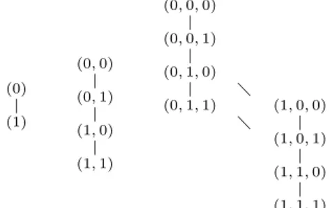
The statement of Proposition 5.2 can be summed up by the following sentence:ksuccessive bisections of the digraphIn lead to the digraphIk. In Fig. 5 this proposition is illustrated for n = 5 and k = 1,2,3. Note that wile the nodes of I5 are binary 5-tuples, the vertices of the corresponding
graphs I1, I2 and I3 are binary 1-tuples, 2-tuples and 3
-tuples, respectively.
(0)
|
(1)
(0,0)
|
(0,1)
|
(1,0)
|
(1,1)
(0,0,0)
|
(0,0,1)
|
(0,1,0)
|
(0,1,1) (1,0,0) |
(1,0,1)
|
(1,1,0)
|
(1,1,1)
Fig. 5. ksuccessive bisections of the digraphInlead to the
digraphIk(n= 5,k= 1,2,3).
Corollary 5.1: Let n ≥ 1 and 1 ≤ k ≤ n. Then the subgraphs I0,⌣...,k 0
n and I1,
k ⌣
...,1
n are the ones with the largest and smallest occurrence probabilities (i.e., sum of the oc-currence probabilities of all nodes lying on each of them), respectively, among all the 2k subgraphsIu¯1,...,u¯k
n obtained
after ksuccessive bisections of In.
Proof: Using Theorem 5.2, we see that proving the current theorem is equivalent to proving that, for all k≥1, the binaryk-tuples
0,. . .,⌣k 0= 0 and 1,. . .,⌣k 1= 2k−1
are the maximum and minimum elements, respectively, in the posetIk. This fact, illustrated by Figs. 2 &3, has been demonstrated in Example 2.5.
VI. CONCLUSION
In this paper, we have considered complex systems de-pending on an arbitrarily large numbernof random Boolean variables, i.e., the so-called complex stochastic Boolean systems (CSBSs). We have defined and characterized by a simple matrix description the intrinsic order between the binary n-tuples associated to a CSBS. Then we have presented the usual graphical representation for CSBSs: a Hasse diagram on2n
nodes called the intrinsic order graph, and denoted by In. New properties of the intrinsic order graph have been stated and proved. These properties deal with different features of the intrinsic order graph like, e.g., its edges; the natural decomposition of the graph In into its 2n−2 “columns of size 4” or congruence chains (mod 4); the shadows, neighbors and degrees of its vertices; and the study of some relevant isomorphic subgraphs of In obtained by bisection. From a theoretical point of view, this paper suggests the search of new graph-theoretic and order-theoretic properties of the intrinsic order graph In. For practical applications, some of these properties can be applied to develop new algorithms that identify binary strings with large occurrence probabilities. Such algorithms can be used in Reliability Theory and Risk Analysis to estimate the failure probability of a technical system modeled by a CSBS.
REFERENCES
[1] R. Diestel,Graph Theory, 3rd ed. New York: Springer, 2005. [2] L. Gonz´alez, “A New Method for Ordering Binary States Probabilities
in Reliability and Risk Analysis,”Lect Notes Comp Sc, vol. 2329, no. 1, pp. 137-146, 2002.
[3] L. Gonz´alez, “N-tuples of 0s and 1s: Necessary and Sufficient
Condi-tions for Intrinsic Order,”Lect Notes Comp Sc, vol. 2667, no. 1, pp. 937-946, 2003.
[4] L. Gonz´alez, “A Picture for Complex Stochastic Boolean Systems: The Intrinsic Order Graph,”Lect Notes Comp Sc, vol. 3993, no. 3, pp. 305-312, 2006.
[5] L. Gonz´alez, “Algorithm Comparing Binary String Probabilities in Complex Stochastic Boolean Systems Using Intrinsic Order Graph,”
Adv Complex Syst, vol. 10, no. Suppl. 1, pp. 111-143, 2007. [6] L. Gonz´alez, “Complex Stochastic Boolean Systems: Generating and
Counting the Binaryn-Tuples Intrinsically Less or Greater thanu,” in
Lecture Notes in Engineering and Computer Science: World Congress on Engineering and Computer Science 2009, pp. 195-200.
[7] L. Gonz´alez, “Partitioning the Intrinsic Order Graph for Complex Stochastic Boolean Systems,” in Lecture Notes in Engineering and Computer Science: World Congress on Engineering 2010, pp. 166-171. [8] L. Gonz´alez, “Ranking Intervals in Complex Stochastic Boolean Sys-tems Using Intrinsic Ordering,” in Machine Learning and Systems Engineering, Lecture Notes in Electrical Engineering, vol. 68, B. B. Rieger, M. A. Amouzegar, and S.-I. Ao, Eds. New York: Springer, 2010, pp. 397410.
[9] L. Gonz´alez, “Complex stochastic Boolean systems: New properties of the intrinsic order graph”, Lecture Notes in Engineering and Computer Science: Proceedings of the World Congress on Engineering 2011, WCE 2011, 6-8 July, 2011, London, U.K., pp. 1194-1199.
[10] L. Gonz´alez, D. Garc´ıa, and B. Galv´an, “An Intrinsic Order Criterion to Evaluate Large, Complex Fault Trees,” IEEE Trans on Reliability, vol. 53, no. 3, pp. 297-305, 2004.
[11] W. G. Schneeweiss,Boolean Functions with Engineering Applications and Computer Programs. New York: Springer, 1989.