www.ann-geophys.net/26/3585/2008/ © European Geosciences Union 2008
Annales
Geophysicae
Spectra and anisotropy of magnetic fluctuations in the Earth’s
magnetosheath: Cluster observations
O. Alexandrova1, C. Lacombe2, and A. Mangeney2
1University of Cologne, Institute of Geophysics and Meteorology, Albertus-Magnus-Platz 1, 50923 Cologne, Germany 2LESIA, Observatoire de Paris, CNRS, UPMC, Universit´e Paris Diderot, 5 place J. Janssen, 92190 Meudon, France Received: 7 May 2008 – Revised: 11 September 2008 – Accepted: 29 September 2008 – Published: 17 November 2008
Abstract. We investigate the spectral shape, the anisotropy of the wave vector distributions and the anisotropy of the am-plitudes of the magnetic fluctuations in the Earth’s magne-tosheath within a broad range of frequencies[10−3,10]Hz which corresponds to spatial scales from∼10 to 105km. We present the first observations of a Kolmogorov-like inertial range of Alfv´enic fluctuations δB⊥2∼f−5/3 in the magne-tosheath flanks, below the ion cyclotron frequencyfci. In the vicinity offci, a spectral break is observed, like in solar wind turbulence. Above the break, the energy of compres-sive and Alfv´enic fluctuations generally follows a power law with a spectral index between−3 and−2. Concerning the anisotropy of the wave vector distribution, we observe a clear change in its nature in the vicinity of ion characteristic scales: if at MHD scales there is no evidence for a dominance of a slab (kk≫k⊥) or 2-D (k⊥≫kk) turbulence, above the spectral
break, (f >fci, kc/ωpi>1) the 2-D turbulence dominates. This 2-D turbulence is observed in six selected one-hour in-tervals among which the average ionβvaries from 0.8 to 10. It is observed for both the transverse and compressive mag-netic fluctuations, independently on the presence of linearly unstable modes at low frequencies or Alfv´en vortices at the spectral break. We then analyse the anisotropy of the mag-netic fluctuations in a time dependent reference frame based on the field B and the flow velocity V directions. Within the range of the 2-D turbulence, at scales[1,30]kc/ωpi, and for anyβ we find that the magnetic fluctuations at a given frequency in the plane perpendicular toBhave more energy along theB×Vdirection. This non-gyrotropy of the fluctua-tions at a fixed frequency is consistent with gyrotropic fluc-tuations at a given wave vector, withk⊥≫kk, which suffer a
different Doppler shift along and perpendicular toVin the plane perpendicular toB.
Correspondence to:O. Alexandrova (alex@geo.uni-koeln.de)
Keywords. Magnetospheric physics (Magnetosheath) – Space plasma physics (Turbulence)
1 Introduction
In the space plasma turbulence, the presence of a mean mag-netic fieldBgives rise to anisotropies with respect to the field direction (k means parallel, and⊥means perpendicular to
B). There are anisotropies both in the intensitiesδB2of the magnetic fluctuations (δB⊥26=δBk2) and in the distribution of their wave vectorsk(k⊥6=kk), i.e., the energy distribution of
the turbulent fluctuations is anisotropic ink-space.
To study the anisotropy of turbulent fluctuations in space plasma, we chose here the Earth’s magnetosheath as a lab-oratory. Downstream of the bow shock, the solar wind plasma slows down, and the plasma density, temperature and magnetic field increase in comparison with the solar wind plasma. The magnetosheath boundaries (bow shock and magnetopause) introduce an important ion temperature anisotropy T⊥>Tk, and therefore linearly unstable waves,
such as Alfv´en Ion Cyclotron (AIC) and mirror modes, are present (see the reviews by Schwartz et al., 1996; Lucek et al., 2005; Alexandrova, 2008). In the vicinity of the bow-shock, anf−1 power law spectrum is observed at frequen-cies below the ion cyclotron frequency,f <fci, (Czaykowska et al., 2001). The power law spectra∼f−5/3, typical of the solar wind inertial range atf <fci, have not been observed in the magnetosheath. However, as in the solar wind, the en-ergy of the magnetic fluctuations follows a power law close to∼f−3 at frequencies f >fci (Rezeau et al., 1999; Cza-ykowska et al., 2001).
where linearly unstable modes are expected (Alexandrova et al., 2004; Sch¨afer et al., 2005; Narita et al., 2006; Narita and Glassmeier, 2006; Constantinescu et al., 2007). Instead, we are interested in permanent fluctuations in the magnetosheath (and not in spectral peaks) which cover a very broad range of frequencies (more than 5 decades), from frequencies well be-lowfcito frequencies much higher thanfci.
These permanent fluctuations within the frequency range [0.35,12.5]Hz, above fci, and for one decade of scale lengths around Cluster separations (∼100 km), have been studied by Sahraoui et al. (2006) using thek-filtering tech-nique. For a relatively short time interval in the inner mag-netosheath (close to the magnetopause) and for a proton beta
βi∼5, the authors show that the wave-vectors of the fluctu-ations are mostly perpendicular to the mean magnetic field
B,k⊥≫kk, and that their frequencyω0in the plasma frame is zero. In the plane perpendicular toB, thek-distribution is non-gyrotropic, more intense and with a well-defined power lawk−8/3in a direction along the flow velocityVwhich was perpendicular to bothBand the normal to the magnetopause for this particular case. The presence of linearly unstable large scale mirror mode during the considered time interval makes the authors conclude that the small scale fluctuations with the observed dispersion propertiesk⊥≫kk and ω0=0 result from a non-linear cascade of mirror modes.
At higher frequencies,∼[10,103]Hz, between about the lower hybrid frequency flh and 10 times the electron cy-clotron frequenciefce, the permanent fluctuations observed in the magnetosheath, during four intervals of several hours, have been studied by Mangeney et al. (2006) and Lacombe et al. (2006). The corresponding spatial scales,∼[0.1,10]km ≃[0.3,30]kc/ωpe(c/ωpebeing the electron inertial length), are much smaller than the Cluster separations, and so only the one-spacecraft technique could be used to analyze the anisotropy of wave vector distributions.
Magnetic fluctuations withkk≫k⊥, usually called “slab
turbulence”, have rapid variations of the correlation function along the field and weak dependence upon the perpendicu-lar coordinates. For the fluctuations withk⊥≫kk, called
“2-D turbulence”, the correlation function varies rapidly in the perpendicular plane, and there is no dependence along the field direction. So, measurements along different directions with respect to the mean field can give the information on the wave vector anisotropy. Under the assumption of con-vected turbulent fluctuations through the spacecraft (i.e., the phase velocityvφ of the fluctuations is small with respect to the flow velocity), these measurements are possible with one spacecraft thanks to the variation of the mean magnetic fieldBdirection with respect to the bulk flowV. WhileVkB, the spacecraft resolve fluctuations withkkB, whenV⊥B, the fluctuations withk⊥Bare measured.
This idea was already used in the solar wind for study-ing the wave vector anisotropies of the Alfv´enic fluctuations in the inertial range (Matthaeus et al., 1990; Bieber et al., 1996; Saur and Bieber, 1999). The authors suppose that the
observed turbulence is a linear superposition of two uncorre-lated components, slab and 2-D, and both components have a power law energy distribution with the same spectral index
s,δB⊥2(kk)∼A1kk−sandδB⊥2(k⊥)∼A2k⊥−s, whereA1andA2 are the amplitudes of slab and 2-D turbulent components, re-spectively. Bieber et al. (1996) propose two independent ob-servational tests for distinguishing the slab component from the 2-D component.
The first test is based on the anisotropy of the power spec-tral density (PSD) of the magnetic fluctuations in the plane perpendicular to B, i.e., on the non-gyrotropy of the PSD at a given frequency in the spacecraft frame: in the case of a slab turbulence withkkB, all the wave vectors suffer the same Doppler shift depending on the angle betweenkandV, and if the spectral power is gyrotropic in the plasma frame, it will remain gyrotropic in the spacecraft frame; in the case of a 2-D turbulence, withk⊥B, if the PSD is gyrotropic in the plasma frame, it will be non-gyrotropic in the spacecraft frame because the Dopler shift will be different ifkis per-pendicular toVand ifkhas a component alongV.
The second test reveals the dependence of the PSD at a fixed frequency on the angle between the plasma flow and the mean field2BV (defined between 0 and 90 degrees): For a PSD decreasing withk(like a power-law, for example), in the case of the slab turbulence, the PSD for a given frequency will be more intense for 2BV=0◦, and therefore, the PSD decreases while2BV increases; for the 2-D turbulence the PSD will be more intense for2BV=90◦, and so it increases with2BV. Using these tests, Bieber et al. (1996) have shown that the subrange[10−3,10−2]Hz in the inertial range of the slow solar wind is dominated by a 2-D turbulence; however, a small percentage of a slab component is present.
Mangeney et al. (2006) proposed a model of anisotropic wave vector distribution without any assumption on the in-dependence of the two turbulence components. In their gy-rotropic model, the wave vector can be oblique with respect to thekand⊥directions. The authors introduce a cone aper-ture of the angleθkBbetweenkandB, as a free parameter of the model. They assume a power law distribution of the total energy of the fluctuations∼k−s, withsindependent onθkB. For a givenk, the turbulent spectrum is modeled by one of the two typical angular distribution∼cos(θkB)µforknearly parallel toBand∼sin(θkB)µforknearly perpendicular to B. For these two distributions, the cone aperture of θkB is about 20◦forµ=10 and 7◦forµ=100. The angleθ
kB can be easily represented through2BV and so the model can be tested with one-spacecraft measurements.
a strongly anisotropic distribution ofk, withθkB=(90±7)◦ (Mangeney et al., 2006). Actually, this model (as well as the tests of Bieber et al., 1996) is valid not only for a power law energy distribution ink, but for any monotone dependence where the energy decreases with increasingk.
Mangeney et al. (2006) have also shown that the varia-tions ofδB2with2BV for a given frequency was not consis-tent with the presence of waves with a non-negligible phase velocityvφ. In other words, if the observed turbulent fluctu-ations are a superposition of waves, theirvφhas to be much smaller than the flow velocity for any wave numberk. This is consistent with the assumption that the wave frequencyω0 is vanishing: the fluctuations are due to magnetic structures frozen in the plasma frame. These results have been obtained in the magnetosheath flanks forf >10 Hz, at electron spatial scales∼[0.3,30]kc/ωpe.
In this paper we extend the study of Mangeney et al. (2006) to frequencies below 10 Hz, for the same time pe-riods in the magnetosheath flanks. As a result, we will cover the largest possible scale range, from electron (∼1 km) to MHD scales (∼105km). At variance with the previous study, we analyse the spectral shapes and anisotropies for parallel (∼compressive)δBk and for transverse (∼Alfv´enic)δB⊥
fluctuations independently. For Alfv´enic fluctuationsδB⊥
we perform the first test of Bieber et al. (1996), i.e., we an-alyze the gyrotropy of the PSD of the magnetic fluctuations in the plane perpendicular toB, at a given frequency, as a function of2BV.
2 Data and methods of analysis
For our study we use high resolution (22 vectors per sec-ond) magnetic field waveforms measured by the FGM in-strument (Balogh et al., 2001). Four seconds averages of the PSD of the magnetic fluctuations at 27 logarithmically spaced frequencies, between 8 Hz and 4 kHz, are measured by the STAFF Spectrum Analyser (SA) (Cornilleau-Wehrlin et al., 1997). Plasma parameters with a time resolution of 4 s are determined from HIA/CIS measurements (R`eme et al., 2001).
2.1 Magnetic spectra and decomposition inδB⊥andδBk
High resolution FGM measurements allow to resolve tur-bulent spectra up to ∼10 Hz. Similar to Alexandrova et al. (2006), we calculate the spectra of the magnetic fluctu-ations in the GSE directions X, Y and Z, using the Morlet wavelet transform. The total power spectral density (PSD) isδB2(f )=Pj=X,Y,ZδBj2(f ). The PSD of the compres-sive fluctuationsδBk2(f )is approximated by the PSD of the modulus of the magnetic field. This is a good approximation when δB2≪B02, whereB0 is the modulus of the magnetic
field at the largest scale of the analysed data set. The PSD of the transverse fluctuations is therefore
δB⊥2(f )=δB2(f )−δBk2(f ). (1) This approach, based on wavelet decomposition, allows the separation ofδB⊥andδBkwith respect to a local mean field, i.e. to the field averaged on a neighbouring scale larger than the scale of the fluctuations. The lower frequency limit of this approach is a scale where the orderingδB2≪B02is no longer satisfied.
The STAFF-SA instrument measures the spectral matrix hδBi(f )δBj(f )i at higher frequencies. Because of a re-cently detected error about the axes directions in the spin plane (O. Santolik, private communication, 2008) we cannot separate parallel and perpendicular spectra at the STAFF-SA frequencies; however we present here the total PSD, the trace of the spectral matrix.
2.2 Anisotropy of thekdistribution
The motion of the plasma with respect to a probe allows a 1-D analysis of the wave vector distribution along the direction ofV, as was discussed in Sect. 1. The 3-D wave vector power spectrumI (k)≡I (k, θkB, ϕk)depends on the wave number k, on the angleθkB betweenkandB, and on the azimuthϕk ofkin the plane perpendicular toB. Ifω0is the frequency of a wave in the plasma rest frame (ω0andωare assumed to be positive), the Doppler shifted frequencyf=ω/2π in the spacecraft frame is given by
ω= |ω0+k·V|. (2)
The trace of the power spectral density at this frequency is
δB2(ω)=A Z
I (k)δ(ω− |ω0+k·V|)dk (3) i.e. the sum of the contributions with differentk.Ais a nor-malisation factor andδthe Dirac function.
The angleθkBcan be considered as depending on the angle θkV betweenk andV, the angle appearing in the Doppler shift frequency, and on the angle2BV betweenBandV(see Eq. 2 of Mangeney et al., 2006). Thus, the variations ofδB2
with2BV for a givenωwill give information aboutI (k). As was discussed in Sect. 1,δB2increases with increasing2BV when the fluctuations havek⊥≫kk(2-D turbulence) and it decreases for a slab turbulence withkk≫k⊥ (see Fig. 6 of Mangeney et al., 2006). As a consequence, in the case of 2-D turbulence, the spectrum of the fluctuations will be higher for large angles2BV than for small ones, and vice-versa for the slab geometry.
2.3 δB-anisotropy in theBV-frame
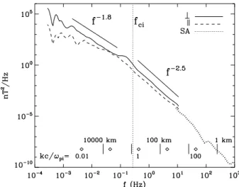
Fig. 1. FGM and STAFF-SA/Cluster data on 19 December 2001, 02:00–04:00 UT. Average spectra of the magnetic fluctua-tions, calculated using the Morlet wavelet transform of the FGM data (f <10 Hz). Solid line: for the transverse fluctuations δB⊥. Dashed line: for the compressive fluctuationsδBk. Dotted line: the
total power spectral density, STAFF-SA data (f >8 Hz). The di-amonds give the scaleskc/ωpi≃krgi≃0.01 to 100. The vertical
dotted line gives the average proton cyclotron frequencyfci. The
shapes of the power lawsf−1.8andf−2.5are shown.
we shall consider the following reference frame (b,bv,bbv):
bis the direction of theBfield,bvthe direction ofB×Vand
bbvthe direction ofB×(B×V).
The definition of this frame depends on the considered scale (frequency). A local reference frame (defined on a neighbouring scale larger than the scale of the fluctuations) is defined for frequencies below the spacecraft spin frequency
fspin=0.25 Hz which limits the plasma moments time reso-lution to 4 s. Then, for any frequencyf >fspin we use the frame (b,bv,bbv) redefined every 4 s.
In this frame, we only consider the frequencies below 10 Hz, i.e., the FGM data (the STAFF-SA data cannot be used because of the error that has to be corrected in the whole data set). We project the wavelet transform ofBX,BY and BZon theb,bv,bbvdirections and we calculate the squares of these projections δBb2(f, t ), δBbv2(f, t ) and δBbbv2 (f, t )
which are the diagonal terms of the spectral matrix in this new frame.
3 k-distribution ofδB⊥andδBk
3.1 A case study withβi≃1
We consider an interval on 19 December 2001, from 02:00 to 04:00 UT. For this interval, the mean plasma parame-ters are the following: the magnetic field B=(18±2)nT, the ion plasma densityNi=(7±1)cm−3, the ion temperature
Ti=(120±15)eV (with Ti⊥/Tik=1.7), the ion plasma beta βi=(1.1±0.4), the ion inertial lengthc/ωpi=(90±5)km and the ion Larmor radius rgi=(65±15)km. The electrons are isotropic and their temperature is small with respect to the ion temperature,Te≃20 eV. The average upstream bow shock an-gleθBNcalculated with the ACE data is about 70◦(Lacombe et al., 2006).
Figure 1 displays the average spectra of the FGM data for the transverse fluctuations (solid lines) and for the compres-sive fluctuations (dashed lines). The total PSD of the STAFF-SA data is the dotted line above 8 Hz. The total covered fre-quency range is more than six decades, from 3×10⁻⁴Hz to 103Hz. The small vertical bars just above the abscissae-axis indicate the scales fromλ=104km to 1 km corresponding to the Doppler shift f=V /λ for θkV=0◦ and for the average velocity V=(246±25)km/s. The diamonds above the ab-scissae indicate the scaleskc/ωpi≃krgi≃0.01 to 100, corre-sponding to the frequencyf=kV /2π. Precisely,kc/ωpi=1 appears in the spectrum atf=(0.44±0.05)Hz and krgi=1 appears atf=(0.63±0.11)Hz.
We see in Fig. 1 that, in the FGM frequency range,
δB⊥2(f )is everywhere larger than δBk2(f ), except around
f∼5×10⁻²Hz whereδB2
⊥∼δB
2
k, and where the
compres-sive fluctuations display a spectral break. The spectrum of
δB⊥ displays a bump and a break around 0.2 Hz, that can
be a signature of Alfv´en vortices (Alexandrova et al., 2006). Below the bump,δB⊥2(f )∼f−1.8, a power law with an expo-nent close to the Kolmogorov’s one−5/3 (in Sect. 5 we will analyse spectral shapes in more details). Above the bump, forkc/ωpi>0.2,δB⊥2(f )andδBk2(f )follow a similar power
law∼f−2.5. This power law extends on the STAFF-SA fre-quency range up tokc/ωpi≃50 (kc/ωpe≃1.2). It is quite possible that, above these scales, the dissipation of the elec-tromagnetic turbulence starts. However, aroundf≃100 Hz, there is another spectral bump, which is due to whistler waves, identified by their right-handed polarisation. The question of the turbulence dissipation is out of scope of the present paper and will be analysed in details in the future.
Now, we consider the anisotropy of the distribution of the wave vectors. Figure 2 shows the dependence ofδB⊥2 (left column) andδBk2 (right column) on the angle 2BV at dif-ferent frequencies. The thick solid curves give the median values for bins 5◦ wide. The upper panels of Fig. 2
cor-respond tof=3 Hz (kc/ωpi≃7). The observed increase of δB⊥2 andδBk2 with2BV can be produced only by fluctua-tions withk⊥≫kk, with phase velocitiesvφnegligible with respect to the plasma bulk velocity, and with decreasing in-tensity of the fluctuations with increasingk(as was discussed in Sects. 1 and 2.2).
Fig. 2. FGM/Cluster data on 19 December 2001, 02:00–04:00 UT. Upper panels: Scatter plots of the power spectral density of the mag-netic fluctuations atf=3 Hz as a function of the angle between the local mean field and velocity,2BV. The distributions of the
en-ergy of Alfv´enic fluctuationsδB⊥2 is shown in the left panel,δBk2is shown in the right panel. Middle and lower panels have the same format, but here the frequencies are respectively 0.52 Hz and 0.2 Hz. In all panels, the thick lines give the median value for bins 5◦wide.
andδBk2at 0.2 Hz (kc/ωpi≃0.5), just at the spectral bump ofδB⊥2 (see Fig. 1). δBk2still increases with2BV (in spite of a large dispersion of the data points around the median), whileδB⊥2 has a flat distribution with2BV. This can be due to several reasons: (i)I (k)is no longer a decreasing func-tion withk, (ii)I (θkB)is more isotropic in the spectral bump and/or (iii) the fluctuations are not frozen in plasma at this scale. This spectral bump, as we have already mentioned, can be the signature of Alfv´en vortices withk⊥≫kk,
propa-gating slowly in the plasma frame. It can be also the signature of propagating AIC waves withkk≫k⊥, which are unstable
for the observed plasma conditions (Mangeney et al., 2006; Samsonov et al., 2007). However, as explained in Sects. 1 and 2.2, the energy of fluctuations withkk≫k⊥ would
de-crease with increasing2BV at a given frequency, while in our caseδB⊥2 seems to be independent on2BV.
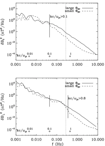
Fig. 3. FGM/Cluster data on 19 December 2001, 02:00–04:00 UT. Average power spectral density of the compressive magnetic fluctu-ations (upper panel) and of the transverse fluctufluctu-ations (lower panel). In each panel, the solid line is the average spectrum for large2BV
angles, and the dashed line for small2BV. The vertical dotted line
gives the averagefci, the diamonds indicatekc/ωpi=0.01, 0.1 and
1.
As we have just seen from Fig. 2 (and as discussed in Sects. 1 and 2.2), the comparison of the energy level of the turbulent fluctuations for different2BV at a given frequency gives us a good estimate of the wave vector anisotropy. We compare now the PSD of the fluctuations observed for large
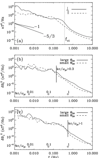
Fig. 4. FGM/Cluster data on 17 May 2002, 08:30–09:30 UT.
(a)Average PSD ofδB⊥( solid line), PSD ofδBk(dashed line),
the vertical dotted line gives the averagefci;(b)the average
spec-trum ofδBkfor large angles2BV (solid line) and for small
an-gles (dashed line), diamonds indicate kc/ωpi=0.01, 0.1 and 1
(krgi=kc/ωpiin this case);(c)same as (b), forδB⊥.
δBk2la≃δBk2sa≃10−4nT2/Hz, that is the sensitivity limit of the FGM instrument. Therefore, the observations atf >5 Hz are not physically reliable.
The lower panel of Fig. 3 displays the spectra for the trans-verse fluctuations for large and small angles 2BV, δB⊥2la (solid line) and δB⊥2sa (dashed line). We observe that
δB⊥2labecomes larger thanδB⊥2saat about the same scale of
kc/ωpi≃0.1 as for compressive fluctuations. However, here within the spectral bump range,∼ [0.1,0.3]Hz, we observe
δB⊥2la≃δB⊥2sa. This is consistent with our previous results that in this short frequency range the 2-D turbulence model is not valid (cf. Fig. 2). A clear dominance ofδB⊥2la over
δB⊥2sa is then observed forf >0.3 Hz (kc/ωpi>0.8, see a vertical solid line).
These observations allow to conclude that, forβi≃1, there is a change in the nature of the wave-vector distribution of the magnetic fluctuations in the magnetosheath, in the vicin-ity of ion characteristic scale: if at MHD scales there is no clear evidence for a dominance of a slab or 2-D geometry of the fluctuations, at ion scales (kc/ωpi>0.1) the 2-D tur-bulence dominates. This is valid for both the Alfv´enic and compressive fluctuations. The large scale limit of the 2-D turbulence is, however, different for Alfv´enic and compres-sive fluctuations, and seems to depend on the presence of spectral features, as peaks or bumps. We analyse this point more in details by considering other cases.
3.2 Other case studies
The comparison between the spectra for large2BV and for small2BV has been made during four other one-hour inter-vals, with different averageβi and different average shock anglesθBN. For the same intervals, Samsonov et al. (2007) display the observed proton temperature anisotropy and the corresponding thresholds for AIC and mirror instabilities.
Figure 4 gives the results of the analysis for an interval (17 May 2002, 08:30–09:30 UT) for which θBN≃70◦, βi=(1.6±0.3), B=(24±3)nT, V=(190±10)km/s, fci=(0.37±0.04)Hz, c/ωpi=(55±2)km and rgi=(50±5)km.
Figure 4a gives the average PSD of transverse (solid line) and compressive fluctuations (dashed line). There is a spec-tral bump for the transverse fluctuations around 0.2 Hz. Be-low the spectral bump,δB⊥2(f )∼f−5/3. For the compressive fluctuations there is a spectral bump around 0.07 Hz, proba-bly made of mirror modes. Below the bump,δBk2(f )is close tof−1.
In the two other panels of Fig. 4, we display the spec-tra for large and small2BV for compressive and for trans-verse fluctuations, respectively. In Fig. 4b, at frequencies above the bump ofδBk2(f >0.1 Hz,kc/ωpi≥0.3) we observe δBk2la>δBk2sa. In Fig. 4c, we observeδB⊥2la≃δB⊥2saat large scales (observed atf <0.05 Hz, i.e.kc/ωpi<0.1), but at fre-quencies above the bump of δB⊥2 (kc/ωpi>1) we observe δB⊥2la>δB⊥2sa. So, the transverse and compressive fluctu-ations have k⊥≫kk at scales smaller than their respective spectral bumps. This confirms the conclusions of Sect. 3.1.
Fig. 5. Same as Fig. 4, but for FGM/Cluster data on 16 December 2001, 05:30–06:30 UT.
In an interval with a larger value of βi (17 May 2002, 11:00–12:00 UT, βi≃4.5, θBN≃73◦), the analysis of the spectra for large and small2BV (not shown) shows that the 2-D turbulence takes place forkc/ωpi>0.3 for the transverse fluctuations, and forkc/ωpi>0.2 for the compressive fluctu-ations. So, the 2-D turbulence range of scales for the trans-verse fluctuations is wider in this case.
Figure 5 shows the results of the analysis for an interval (16 December 2001, 05:30–06:30 UT) downstream of an oblique bow shock (θBN≃50◦), when βi=(10±3), B=(27±6)nT, V=(370±20)km/s, fci=(0.4±0.1)Hz, c/ωpi=(30±2)km andrgi=(60±20)km. The wavenumber kc/ωpi=1 appears in the spectrum atf=(2.0±0.2)Hz and the wavenumberkrgi=1 appears atf=(1.1±0.3)Hz.
Figure 5b shows that at low frequencies (i.e., at large scales, kc/ωpi<0.1) the spectrum for large angle δBkla dominates slightly at every frequencies. At smaller scales,
kc/ωpi>0.1, this dominance is more clear. Figure 5c shows
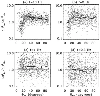
Fig. 6. FGM/Cluster data on 19 December 2001, 02:00–04:00 UT. Scatter plots of the ratioR=δBbv2 /δBbbv2 averaged over 4 s, as a function of the angle 2BV at(a) 10 Hz,(b) 3 Hz, (c) 1 Hz and
(d)0.3 Hz. The thick lines give the median value for bins 10◦wide.
that δB⊥la>δB⊥sa as far as kc/ωpi>0.01 (wavelengths smaller than 104km), i.e., theδB⊥fluctuations can be
de-scribed by the 2-D-turbulence model at all the scales smaller than the Earth’s radius. In this case, with large value of plasma beta, the 2-D turbulence range of scales increases again, but the lower limit of 2-D turbulence is not related to any spectral features, as was observed for smallerβi.
We may therefore conclude that, at frequencies above the spectral break in the vicinity offci, theδB⊥ andδBk
fluc-tuations in the magnetosheath havekmostly perpendicular toB, and this is independent onβi and onθBN. In terms of spatial scales, this is valid forkc/ωpi>0.1 (or>1 when spectral features appear in the vicinity of kc/ωpi=1). For high values ofβi, the range of scales of the 2-D turbulence seems to increase: forβi∼10 the fluctuations havek⊥≫kk forkc/ωpi>0.01. This small scale spectral anisotropy is also independent on the presence of transverse and/or compres-sive spectral features (peaks) at larger scales. Nevertheless, for the moderate values of beta (βi<3), these spectral peaks appear as the lower limit of 2-D turbulence.
4 Gyrotropy of the magnetic fluctuations
In this section we analyse the anisotropy of the amplitudes of magnetic fluctuations in the plane perpendicular toB. For this purpose, we use the coordinate frame based onBandV,
For the same time interval as Fig. 1, Fig. 6 displays the ra-tioR=δBbv2/δBbbv2 , amplitude of the fluctuations alongB×V
over the amplitude alongB×(B×V), in the plane perpendic-ular toB, at four fixed frequencies, as a function of2BV.
In Fig. 6a (f=10 Hz,kc/ωpi=23) and Fig. 6b (f=3 Hz, kc/ωpi=7) the ratioR is larger than 1 for2BV&20◦. The median value decreases and reaches 1 or less for2BV<20◦. A similar dependence was observed by Bieber et al. (1996) and Saur and Bieber (1999) at MHD scales in the solar wind, indicating the dominance of the 2-D turbulence.
At larger scales (Fig. 6c,f=1 Hz,kc/ωpi=2), in spite of the strong dispersion of R, the median values are slightly larger than 1 for any2BV: the 2-D turbulence still domi-nates. At an even larger scale, the scale of the spectral break (Fig. 6d,f=0.3 Hz,kc/ωpi=0.7), the ratioRis strongly dis-persed. The variation of the median does not correspond to a slab or 2-D turbulence. That is in agreement with the re-sults obtained within the spectral break frequency range in Sect. 3.1 (cf. Fig. 2, lowest panel forδB⊥).
The anisotropy of the magnetic fluctuations for the [10−3,10]Hz frequency range is shown in Fig. 7 with aver-age spectra in the three directionsb(dashed line),bv(solid line) andbbv(dotted line). The panels (a) to (f) correspond to increasing values ofβi for the six considered intervals. For each interval, the vertical solid bar indicates the scale
kc/ωpi=1, the dashed-dotted bar indicateskrgi=1 and the dotted bar showsfci.
In Fig. 7a, b and c, for kc/ωpi≥1 we observe that the spectra of the components alongband alongbbvare nearly equal,δBb2≃δBbbv2 . In Fig. 7e and f,δBb2is larger thanδBbv2 : the fluctuations are more compressive for the largest values of βi. All the panels of Fig. 7 show thatδBbv2 >δBbbv2 for kc/ωpi≥1 (krgi≥1). So, within the 2-D turbulence range the PSD is not gyrotropic at a given frequency.
As we have mentioned in Sect. 1, the observed non-gyrotropy in the spacecraft frame can be due to the Doppler shift. Indeed, we have shown in Sect. 3 that the wave vectors
kare mainly perpendicular toB, i.e.klies in plane spanned bybvandbbv. Assuming plane 2-D turbulence, the relation
k⊥·δB=0 holds and thus, the wave vectors along bbv(i.e.,
along the direction of the flow in the plane perpendicular to
B, we denote such wave vectorskbbv) contribute to the PSD ofδBbvand the wave vectors alongbv(kbv) contribute to the PSD ofδBbbv. Even ifI (k)is gyrotropic, the fluctuations δBbv withkbbvsuffer a Doppler shift stronger than the fluc-tuationsδBbbv withkbv. For 2-D turbulence, this Doppler shift effect is more pronounced when2BV reaches 90◦.
This implies that, for a gyrotropic energy distribution,
I (kbv)≃I (kbbv), in the plane perpendicular to B, and if the energy decreases with k, for example as a power law
I (k)∼k−s, the observed frequency spectrumδBbv2 (f )will be more intense thanδBbbv2 (f ). In other words, at the same fre-quencyfin the spacecraft frame, we observe the fluctuations with|kbv|>|kbbv|. As the larger wave numbers correspond
to a weaker intensity (for a monotone energy decrease with
k),δBbbv2 will be smaller thanδBbv2.
Therefore, the non-gyrotropy of δB2(f ), observed here, could be due to the non-gyrotropy of the Doppler shift, and could be compatible with a gyrotropic distribution ofI (k). This is confirmed by the upper panels of Fig. 6: as far ask
is mainly perpendicular toB, the Doppler shift is small and gyrotropic for small2BV and we observeR∼1, i.e. the PSD is gyrotropic; but for large2BV,R>1.
On the other hand, the ratioR(f )>1, observed in Fig. 6a and b for 2BV≃90◦, is also compatible with the non-gyrotropick-distribution observed by Sahraoui et al. (2006) near the magnetopause, for2BV≃90◦. In this case study, the authors show that the turbulent cascade develops along
V, perpendicular toB andn, wheren is the normal to the magnetopause. In this geometry, the direction V is close tobbv. Therefore, a non-gyrotropic I (k)distribution with
δBbv2 (k)/δBbbv2 (k)>1 is expected in the k-domain. This non-gyrotropy of wave vectors is then reinforced by the Doppler shift, and would giveδBbv2 (f )/δBbbv2 (f )>1 in the
f-domain.
5 Spectral shapes
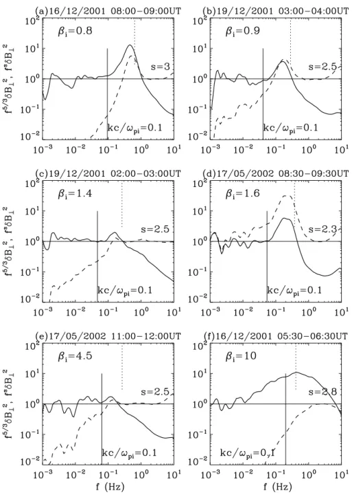
We have mentionned in Sect. 3 that, at frequenciesf <fci, below the spectral break, the spectra of the transverse fluctu-ationsδB⊥2(f )follow a power law close tof−5/3(see Figs. 1 and 4a). For the six intervals of Fig. 7, Fig. 8 displays com-pensated plots of the transverse spectraf5/3δB⊥2(f )(solid lines). On the low frequency side of these plots, we see that the compensated spectra oscillate around a horizontal line, in a frequency range which varies slightly from day to day: a power lawf−5/3 is thus a good approximation for the ob-servations in this frequency range. In Fig. 8a to e, for which
βi is between 0.8 and 4.5, the Kolmogorofff−5/3power law is observed below 0.06 or 0.1 Hz, corresponding to scales
kc/ωpi<0.1 (see the vertical solid bar).
In Fig. 8f, forβi≃(10±3), thef−5/3power law is only ob-served below 0.01 Hz, i.e., below the 2-D turbulence range of δB⊥ (see Fig. 5c). Above this frequency, as we see in
Fig. 7f, the spectra of all the components are close to an
f−1 power law and the three spectra have nearly the same intensity,δBb2(f )≃δBbv2 (f )≃δBbbv2 (f ). This isotropy of the amplitudes of the turbulent fluctuations is natural to observe in a high beta plasma, where the mean magnetic field does not play any important role. Within this frequency range the spectrum can be also formed by a superposition of AIC and mirror waves. For such highβi, the mirror modes are more unstable than the AIC waves, but they have an impor-tant Alfv´enic component (G´enot et al., 2001), that can also contribute to make fluctuations more isotropic.
Abovefci, the spectraδBk2(f )andδB⊥2(f )follow similar power laws, see Fig. 7. The compensated spectrafsδB⊥2(f )
Fig. 7. Average spectra of the magnetic fluctuations in the(b,bv,bbv)-frame,bis parallel to theBfield (dashed line),bvis parallel to
B×V(solid line),bbvis parallel toB×(B×V)(dotted line). For each of the 6 considered one-hour intervals a vertical dotted bar givesfci,
a vertical solid bar gives the Doppler shifted wavenumberkc/ωpi=1 and a dashed-dotted bar giveskrgi=1. In each panel the shapes of the
power lawsf−5/3,f−1are indicated; in the high frequency range we show thef−sspectral shape, withsdetermined in Sect. 5, see Fig. 8.
lines. We see that the compensated spectraf2.5δB⊥2(f ) os-cillate around a horizontal line in a few cases (Fig. 7b, c and e), for different values ofβi. In Fig. 8a, the power law is steeper,s=3. Actually, in this case the spectral bump is the most clearly pronounced of the six analyzed intervals. This bump is a signature of the Alfv´en vortices, which have their own spectrum∼k−4ork−6, depending on the vortex
Fig. 8. Compensated spectraf5/3δB⊥2(f )(solid lines) andfsδB2⊥(f )withsindicated in each panel (dashed lines) for the same time periods as Fig. 7.
6 Summary and discussion
In the present paper, we have analysed six one-hour intervals in the middle of the terrestrial magnetosheath (at more than one hour from the crossing of the bow shock or of the netopause). Precisely, we considered intervals in the mag-netosheath flanks: the local times for the three considered days are respectively 08:00, 17:00 and 18:00 h (Lacombe et al., 2006). The ion beta varies from one interval to another,
βi∈[0.8,10], that allows us to study the plasma turbulence in a very large range of plasma conditions.
6.1 Spectral shape
The spectral shape of the magnetic fluctuations in the mag-netosheath has been studied by several authors (see Alexan-drova, 2008). Rezeau et al. (1999) find a power lawf−3.4
power laws aroundf−1belowf
ci, andf−2.6abovefci. But in these studies, intervals of 4 min have been analyzed, so the minimal resolved frequency is about 10−2Hz. In the present paper, the length of the intervals allows to reach frequencies smaller than 10−3Hz.
Here, we present, for the first time, the observations of a Kolmogorov-like inertial range for Alfv´enic fluctuations
δB⊥2(f )∼f−5/3in the frequency rangef <fci. It is clearly observed in five of the six studied intervals, those for which
βi<5 and when Alfv´enic fluctuations were dominant. Such a Kolmogorov power law is observed in the Alfv´enic inertial range of the solar wind turbulence, below the spectral break in the vicinity offci. The presence of such power law in the magnetosheath flanks is consistent with the estimations made by Alexandrova (2008): in the flanks, the transit time of the plasma is longer than in the subsolar regions, and it is much longer than the time of nonlinear interactions; therefore, the turbulence has enough time to become developed.
In the high frequency range,f >fci, we generally observe δB⊥2(f )andδBk2(f )following similar power lawf−swith a spectral indexsbetween 2 and 3, in agreement with previous studies.
6.2 Wave-vector anisotropy
We analysed here the anisotropy of wave-vector distribution of the magnetic fluctuations from 10−3to 10 Hz. This fre-quency range corresponds to the spatial scales going from ∼10 to 105km (from electron to MHD scales). For this anal-ysis we used a statistical method, based on the dependence of the observed magnetic energy at a given frequency on the Doppler shift for different wave vectors (Bieber et al., 1996; Horbury et al., 2005; Mangeney et al., 2006).
Within the inertial range of the magnetosheath turbulence (f <fci,kc/ωpi<1,krgi<1), we do not observe a clear ev-idence of wave-vector anisotropy. It can be related to the fact that linearly unstable modes, such as AIC modes with
kmainly parallel toBand mirror modes withkmainly per-pendicular toB, together with Alfv´en vortices withk⊥≫kk
co-exist in this frequency range.
However, above the spectral break in the vicinity of the ion characteristic scales (f >fci,kc/ωpi>1,krgi>1 and up to electron scales), we observe a clear evidence of 2-D turbu-lence withk⊥≫kkfor bothδB⊥andδBk, and independently
onβi, on the bow-shock geometryθBN, and on the wave ac-tivity within the inertial range at larger scales. This wave vector anisotropy seems to be a general property of the small scale turbulence in the Earth’s magnetosheath.
The range of wavenumbers of this 2-D turbulence some-times goes down tokc/ωpi≃0.1 (or even tokc/ωpi≃0.01), but usually it is limited bykc/ωpi≃1, while atkc/ωpi<1 spectral features (peaks or bumps) appear. As we can con-clude from the work of Mangeney et al. (2006), the largest wavenumbers of the 2-D turbulence are observed around
kc/ωpi∼100, where the dissipation of electromagnetic
tur-bulence begins. This last conjecture must be verified by a deeper analysis.
6.3 Anisotropy of magnetic fluctuations
Analyzing the anisotropy of the amplitudes of turbulent fluc-tuations, we usually find thatδB⊥2>δBk2; but for the largest plasma βi, the fluctuations are more isotropic δB⊥2∼δBk2. This is valid for both the large scale inertial range and the small scale 2-D turbulence. The dominance ofδBk2happens only locally in the turbulent spectrum, indicating the pres-ence of an unstable mirror mode.
Concerning the gyrotropy of the amplitude of the mag-netic fluctuations in the plane perpendicular toB, there is no universal behavior at large scales. At smaller scales, within the frequency range[0.3−10]Hz and for anyβi, the 2-D tur-bulence is observed to be non-gyrotropic: the energy δBbv2
along the direction perpendicular toVandBis larger than the energyδBbbv2 along the projection ofVin the plane per-pendicular toB. This non-gyrotropy might be a consequence of different Doppler shifts for fluctuations withkparallel and perpendicular toVin the plane perpendicular toB. The non-gyrotropy at a fixedf is compatible with gyrotropic fluctu-ations at a givenk. On the other hand such a non-gyrotropy will be also observed if thek-distribution is not gyrotropic, but is aligned with the plasma flow, as was observed by Sahraoui et al. (2006) in the vicinity of the magnetopause. Acknowledgements. We thank Jean-Michel Bosqued for providing the CIS/HIA proton data, and Nicole Cornilleau-Wehrlin for the STAFF-SA data. We thank Joachim Saur for constructive com-ments on the paper. We are very grateful to the team of the Cluster Magnetic field investigation, to the team of the STAFF instrument, and to the Cluster Active Archive (CAA/ESA).
Topical Editor R. Nakamura thanks two anonymous referees for their help in evaluating this paper.
References
Alexandrova, O.: Solar wind vs magnetosheath turbulence and Alfv´en vortices, Nonlin. Processes Geophys., 15, 95–108, 2008, http://www.nonlin-processes-geophys.net/15/95/2008/.
Alexandrova, O., Mangeney, A., Maksimovic, M., Cornilleau-Wehrlin, N., Bosqued, J.-M., and Andr´e, M.: Alfv´en vor-tex filaments observed in the magnetosheath downstream of a quasi-perpendicular bow shock, J. Geophys. Res., 111, A12208, doi:10.1029/2006JA011934, 2006.
Alexandrova, O., Mangeney, A., Maksimovic, M., Lacombe, C., Cornilleau-Wehrlin, N., Lucek, E. A., D´ecr´eau, P. M. E., Bosqued, J.-M., Travnicek, P., and Fazakerley, A. N.: Cluster ob-servations of finite amplitude Alfv´en waves and small-scale mag-netic filaments downstream of a quasi-perpendicular shock, J. Geophys. Res., 109, A05207, doi:10.1029/2003JA010056, 2004. Balogh, A., Carr, C. M., Acu˜na, M. H., et al.: The Cluster Magnetic Field Investigation: overview of in-flight performance and initial results, Ann. Geophys., 19, 1207–1217, 2001,
Bieber, J.W., Wanner, W., and Matthaeus, W. H.: Dominant two-dimensional solar wind turbulence with implications for cosmic ray transport, J. Geophys. Res., 101, 2511–2522, 1996. Constantinescu, O. D., Glassmeier, K.-H., D´ecr´eau, P. M. E., Fr¨anz,
M., and Fornac¸on, K. H.: Low frequency wave source in the outer magnetosphere, magnetosheath, and near Earth solar wind, Ann. Geophys., 25, 2217–2228, 2007,
http://www.ann-geophys.net/25/2217/2007/.
Czaykowska, A., Bauer, T. M., Treumann, R. A., and Baumjohann, W.: Magnetic fluctuations across the Earth’s bow shock, Ann. Geophys., 19, 275–287, 2001,
http://www.ann-geophys.net/19/275/2001/.
G´enot, V., Schwartz, S. J., Mazelle, C., Balikhin, M., Dunlop, M., and Bauer, T. M.: Kinetic study of the mirror mode, J. Geophys. Res., 106, 21 611, doi:10.1029/2000JA000457, 2001.
Horbury, T. S., Forman, M. A., and Oughton, S.: Spacecraft ob-servations of solar wind turbulence: an overview, Plasma Phys. Controlled Fusion, 47, B703–B717, 2005.
Lacombe, C., Samsonov, A. A., Mangeney, A., Maksimovic, M., Cornilleau-Wehrlin, N., Harvey, C. C., Bosqued, J.-M., and Tr´avn´ıˇcek, P.: Cluster observations in the magnetosheath: 2. In-tensity of the turbulence at electron scales, Ann. Geophys., 24, 3523–3531, 2006,
http://www.ann-geophys.net/24/3523/2006/.
Lucek, E. A., Constantinescu, D., Goldstein, M. L., Pickett, J. S., Pinc¸on, J.-L., Sahraoui, F., Treumann, R. A., and Walker, S. N.: The Magnetosheath, Space Sci. Rev., 118, 95–152, 2005. Mangeney, A., Lacombe, C., Maksimovic, M., Samsonov, A. A.,
Cornilleau-Wehrlin, N., Harvey, C. C., Bosqued, J.-M., and Tr´avn´ıˇcek, P.: Cluster observations in the magnetosheath: 1. Anisotropy of the wave vector distribution of the turbulence at electron scales, Ann. Geophys., 24, 3507–3521, 2006,
http://www.ann-geophys.net/24/3507/2006/.
Narita, Y., Glassmeier, K.-H., Fornac¸on, K. H., Richter, I., Sch¨afer, S., Motschmann, U., Dandouras, I., R`eme, H., and Georgescu, E.: Low-frequency wave characteristics in the upstream and downstream regime of the terrestrial bow shock, J. Geophys. Res., 111, A01203, doi:10.1029/2005JA011231, 2006.
Narita, Y. and Glassmeier, K.-H.: Propagation pattern of low fre-quency waves in the terrestrial magnetosheath, Ann. Geophys., 24, 2441–2444, 2006,
http://www.ann-geophys.net/24/2441/2006/.
R`eme, Aoustin, H. C., Bosqued, J. M., et al.: First multispacecraft ion measurements in and near the Earth’s magnetosphere with the identical Cluster ion spectrometry (CIS) experiment, Ann. Geophys., 19, 1303–1354, 2001,
http://www.ann-geophys.net/19/1303/2001/.
Rezeau, L., Belmont, G., Cornilleau-Wehrlin, N., and Reberac, F.: Spectral law and polarization properties of the low frequency waves at the magnetopause, Geophys. Res. Lett., 26, 651–654, 1999.
Sahraoui, F., Belmont, G., Rezeau, L., Cornilleau-Wehrlin, N., Pinc¸on, J. L., and Balogh, A.: Anisotropic tur-bulent spectra in the terrestrial magnetosheath as seen by the Cluster spacecraft, Phys. Rev. Lett., 96, 075002, doi:10.1103/PhysRevLett.96.075002, 2006.
Samsonov, A. A., Alexandrova, O., Lacombe, C., Maksimovic, M., and Gary, S. P.: Proton temperature anisotropy in the magne-tosheath: comparison of 3-D MHD modelling with Cluster data, Ann. Geophys., 25, 1157–1173, 2007,
http://www.ann-geophys.net/25/1157/2007/.
Saur, J. and Bieber, J. W.,: Geometry of low-frequency solar wind magnetic turbulence: Evidence for radially aligned Alf´enic fluc-tuations, J. Geophys. Res., 104, 9975–9988, 1999.
Sch¨afer, S., Glassmeier, K.-H., Narita, Y., Fornac¸on, K. H., Dan-douras, I., and Fr¨anz, M.: Statistical phase propagation and dis-persion analysis of low frequency waves in the magnetosheath, Ann. Geophys., 23, 3339–3349, 2005,
http://www.ann-geophys.net/23/3339/2005/.