Assessing wheat performance using environmental information

(1)

______________________________

Corresponding author: Dejan Dodig, Maize Research Institute Zemun Polje, Slobodana Baji a 1, 11185 Belgrade, Serbia, e-mail: [email protected]

UDC 575: 633.11

Original scientific paper

ASSESSING WHEAT PERFORMANCE USING ENVIRONMENTAL INFORMATION

Dejan DODIG1_{, Miroslav ZORI} 2_{, Desimir KNEŽEVI} 3_{, Bojana}

DIMITRIJEVI 2_{and Gordana ŠURLAN–MOMIROVI} 2

1_{Maize Research Institute Zemun Polje, Belgrade} 2 _{Institute of Field Crop Science, Faculty of Agriculture, Belgrade}

3 _{Faculty of Agriculture, University of Priština, Zubin Potok}

Dodig D., M. Zori , D.Kneževi , B.Dimitrijevi and G. Šurlan Momirovi (2007): Assessing wheat performance using environmental information. – Genetika, Vol. 39, No. 3, 413-425.

(2)

wheat landraces are able to better exploit environments with higher temperatures and lower water availability during vegetative growth (March-June) than cultivars.

Key word: biomass, GEI, grain yield, PLS regression, wheat

INTRODUCTION

Grain yield is a major selection criterion for improved adaptation to environmental stresses in many wheat breeding programs. It is commonly limited by seasonal rainfall, rainfall distributions and temperature. Many studies have assessed interactions of a genotype and a production environment on wheat grain yield (ANNICCHIARICO, 1997; VARGAS et al., 2001; LILLEMO et al., 2004; KAYA et al., 2006). On the other hand, several studies established the importance of total biomass to increase yield in wheat (REYNOLDS et al., 1999; SHEARMAN et al.,

2005), especially in drought stress conditions (van GINKEL et al., 1998; QUARRIE et

al., 1999; DODIG, 2005).

Wheat in Serbia is mainly grown under varied rainfed and water stress conditions. With predicted climate change in southern Europe (WAGGONER, 1993)

the frequency of dry years, and therefore drought will increase. Beside the decrease in yield, the most important consequence of drought is the increase in genotype × environment interaction (GEI) (BLUM, 1988). GEI is described as the differential response of cultivars to environmental changes. An understanding of the environmental causes is of fundamental importance for understanding GEI, for assessing the association between phenotypic and genotypic values, and for enhancing the selection of superior and stable genotypes (CROSSA et al., 1999).

GEI has been studied, described, and interpreted by means of several statistical models (CROSSA, 1990). When additional information on external

environmental variables such as meteorological data or soil variables is available the partial least square (PLS) regression (AASTVEIT and MARTENS, 1986) can be

used to determine which of these variables influence GEI. VARGAS et al. (1999)

studying advantages and/or disadvantages of several statistical models for studying and interpreting GEI with a large number of external and/or cultivar variables in wheat trials. Results of their study indicated that PLS regression model was effective in detecting the environmental variables that explained a sizeable proportion of GEI variability.

(3)

MATERIAL AND METHODS

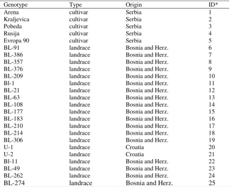
The data set used in this study represents total biomass per plant (g) and grain yield (kg ha-1_{) of 20 wheat landraces and 5 wheat cultivars (Table 1) tested}

for 4 yr (1998-2001) under three treatments: fully irrigated plots (IP), rainfed plots (RP) and under a rain-out plot shelter (drought plots-DP). In this study we included only RP and DP treatments. The rain-out shelter was erected above the plots at the end of the winter period (end of February-beginning of March) when most of the genotypes were at the tillering stage. Amounts of precipitation (mm) during the vegetative period (March-June) were 205.4, 263.3, 74.6 and 284.4 for 1998-2001, respectively. The sowing dates were 1 November 1997, 28 October 1998, 26 October 1999, and 21 October 2000. In each year, the experiment was set up in a randomized complete block design with three replicates. In the first two years, each genotype was sown in a single 1 m row at 20 cm spacing in three replications, with a sowing rate of 60 seeds per row. In the second two years, plots consisted of three 1 m long rows at 20 cm spacing in three replications, with a sowing rate of 80 seeds per row.

Table 1. Genotype name, type and country origin of the genotypes grown in rainfed and drought trials over 4 year (1997-2001)

Genotype Type Origin ID*

Arena cultivar Serbia 1

Kraljevica cultivar Serbia 2

Pobeda cultivar Serbia 3

Rusija cultivar Serbia 4

Evropa 90 cultivar Serbia 5

BL-91 landrace Bosnia and Herz. 6

Bl-1 landrace Bosnia and Herz. 11

U-1 landrace Croatia 20

U-2 landrace Croatia 21

Bl-11 landrace Bosnia and Herz. 22

(4)

The dependent variable (biomass per plant and grain yield) Y matrix was

of size 8 × 25 (8 rows corresponding to treatments and 25 columns corresponding to cultivars). There were 21 explanatory covariables in the Zmatrix of size 8 × 21

(treatments × environmental factors): mean minimum temperature [°C] (mT), mean maximum temperature [°C] (MT), mean soil moisture in the top 75 cm [%] (sm), mean sun hours per day (sh), mean maximum soil temperature at 5 cm [°C] (mst) and winter period (December-February) precipitation [mm] (wpp). All covariables (except wpp) were measured during the growth cycle in March (3), April (4), May (5) and June (6).

Table 2. Values of environmental covariables (Cov) by treatment (RP-rainfed plots and DP-drought plots) in period 1998-2001

Treatment

Cov. DP98 DP99 DP00 DP01 RP98 RP99 RP00 RP01

MT3† _14.5 _15.0 _15.9 _15.6 _12.5 _13.3 _14.6 _14.5

MT4 22.2 21.9 24.8 19.1 19.6 18.9 22.3 18.0

MT5 26.9 27.8 31.4 28.2 23.4 23.8 28.1 24.4

MT6 34.5 33.8 37.2 32.7 28.5 26.7 34.2 27.7

mT3 -1.0 1.5 -0.3 3.5 -1.9 0.8 -1.2 2.7

mT4 6.0 6.3 6.6 5.4 4.8 5.0 5.2 3.5

mT5 9.5 10.3 9.7 10.5 9.1 9.4 9.0 9.5

mT6 14.1 14.8 12.6 12.9 12.9 13.4 11.6 11.7

sm3 21.6 21.9 18.8 21.1 21.2 20.9 18.4 19.5

sm4 21.8 21.4 19.3 19.2 19.8 18.8 16.3 17.4

sm5 21.6 20.1 17.3 17.2 18.4 17.4 13.8 15.8

sm6 19.0 17.8 15.9 14.8 14.6 13.8 12.2 13.3

sh4 6.3 4.6 5.6 4.1 6.3 4.6 5.6 4.1

sh5 5.7 4.9 6.6 4.5 5.7 4.9 6.6 4.5

sh6 5.9 7.0 10.0 6.9 5.9 7.0 10.0 6.9

sh7 9.4 7.4 10.4 7.9 9.4 7.4 10.4 7.9

mst3 9.4 9.7 11.2 13.4 9.4 9.7 11.2 13.4

mst4 18.2 17.2 24.6 18.2 18.2 17.2 24.6 18.2

mst5 24.6 25.2 34.7 28.7 24.6 25.2 34.7 28.7

mst6 33.8 32.5 43.5 30.7 33.8 32.5 43.5 30.7

wpp 142 81 137 64 142 81 138 64

† _{MT, mean maximum temperature; mT, mean minimum temperature; sm, mean soil moisture in the top}

75 cm; sh, mean sun hours per day; mst, mean maximum soil temperatures at 5 cm; wpp, winter period precipitation (December-February); 3, March; 4, April; 5, May; 6, June.

Based on two data matrix Y and Z (which is previously double-centred i.e.

column centred) we applied the partial least square (PLS) regression model (AASTVEIT and MARTENS, 1986; TALBOT and WHEELWRIGHT, 1989; VARGAS et al., 1998). The general idea of this procedure is to relate several Y variables to

several Z variables (AASTVEIT and MARTENS, 1986). In the context of plant

breeding trials Y matrix represented grain yield or biomass per plant data several

(5)

represented additional information (about environments or genotypes) collected during this trials. Both data matrices can be expressed as:

Y = TQ' + F and Z = TP' + E.

where matrix T contains the Z scores; matrix P contains the Z loadings; matrix Q

contains the Y loadings and F and E is the residual of variation. VARGAS et al. (1998) stated that the relationship between Yand Zis transmitted through the latent

variables (or dimensions) T. The number of latent variables (T), which optimally

predict variation in the Y matrix, is determined using cross validation procedure (STONE, 1974). Results of the PLS procedure will be presented using the biplot graph (GABRIEL, 1971) and interpreted by means of the “inner-product” principle (KROONENBERG, 1995). The partial least squares regression procedure was performed using Statistica 7.1 software (StatSoft, Inc. 2004).

RESULTS AND DISCUSSION

For both biomass per plant and grain yield, the analysis of variance showed that the genotype × treatment interaction was highly significant (P<0.001). The main effect of treatments explained 67 and 34% of the total sum of squares, whereas differences between genotype means contributed 14 and 45% and the genotype × treatment interaction 19 and 21% for biomass per plant and grain yield, respectively (data not shown). The cross-validation procedure for the number of significant dimensions suggests that only one dimension (latent vector) out of eight possible is of relevance for prediction.

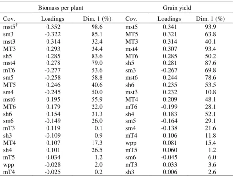
Biomass per plant. - Results from the PLS procedure showed that the first and second dimensions explained 31.6 and 13.5% of the GEI in Y for biomass

(6)

Table 3. Proportion of total variance of X covariables (Cov) explained by the first dimension (Dim. 1) and loadings of X environmental covariables with first dimension

Biomass per plant Grain yield

Cov. Loadings Dim. 1 (%) Cov. Loadings Dim. 1 (%)

mst5† _0.352 _98.6 _mst5 _0.341 _93.9

sm3 -0.322 85.1 MT5 0.321 63.8

mst3 0.314 32.4 MT3 0.314 40.1

MT3 0.293 34.4 mst4 0.307 93.4

sh5 0.285 83.6 MT6 0.285 50.2

mst4 0.278 79.0 sh5 0.281 87.6

mT6 -0.277 53.6 sm3 -0.267 69.8

sm5 -0.258 58.8 mst6 0.244 78.6

MT5 0.246 40.6 sh6 0.235 53.5

sm4 -0.245 50.0 mst3 0.232 10.8

mst6 0.195 55.9 MT4 0.209 48.1

MT6 0.179 22.0 mT6 -0.199 28.1

sh6 0.154 31.3 sh4 0.183 52.1

sm6 -0.149 26.0 sm5 -0.164 29.1

mT3 0.119 0.1 sm4 -0.138 21.6

sh3 -0.109 0.9 mT4 0.106 11.8

MT4 0.107 17.3 wpp 0.081 15.4

sh4 0.101 26.5 mT5 0.060 1.2

mT5 0.034 1.2 sm6 -0.045 6.0

wpp -0.028 2.0 mT3 0.033 3.6

mT4 -0.025 0.2 sh3 0.006 2.6

† _{MT, mean maximum temperature; mT, mean minimum temperature; sm, mean soil moisture in the top}

75 cm; sh, mean sun hours per day; mst, mean maximum soil temperatures at 5 cm; wpp, winter period precipitation (December-February); 3, March; 4, April; 5, May; 6, June.

(7)

June (sh4, sh5, and sh6), and minimum temperature in March and May (mT3 and mT5) (with positive first dimension loadings). The environmental covariables that are located farther from the centre of the PLS biplot caused larger GEI. The smallest contribution to the GEI for biomass per plant had minimum temperature in April (mT4) (Figure 1a).

In general, the years with higher biomass per plant (1998 and 1999) in both treatments had more precipitation during winter period and higher soil moisture in top 75 cm during entire vegetative growth than the remaining two years. The years with lower biomass per plant (2000 and 2001) in both treatments were characterized by high maximum air and soil temperatures. Slightly more tested genotypes had a positive interaction with treatments in 1998 and 1999 than with treatments in the second two years (13 vs. 12). Most genotypes are concentrated in the upper left quadrant of the biplot and had a positive biomass interaction with relatively cool and wet year such as 1998. Only a few genotypes had a high positive biomass interaction with the warm and dry year 2000 (6, 11, and 19). CROSSA et al. (1999) found maximum temperature as most important covariable for explaining GEI for biomass in maize.

The first dimension clearly separates 10 landraces with the highest mean biomass over treatments (25, 24, 23, 16, 13, 22, 14, 17, 21, and 15) from 10 landraces with the lowest mean biomass over treatments (18, 10, 6, 19, 20, 9, 11, 7, 8, and 12). Landraces with high biomass were favoured by good water status during the entire vegetative growth and sun hours in March (tillering stage) and/or maximum temperature in June (grain filling). Low biomass landraces 6, 11, and 19 were less sensitive to high soil and moisture temperatures from April to June in RP00 and DP00. The positive interaction between low biomass landraces 18, 10, 20, 9, 7, 8 and 12 with RP01 and DP01 seems to be due to higher minimum and maximum temperatures in March and May. Cultivars also showed different sensitivity to treatments. Cultivars 1 and 3 were favoured by mT6 and soil moisture from March to June. This led to higher biomass in DP99 and RP99, respectively. Cultivar 5 had high biomass in RP98 probably because of higher sh3 and wpp. Cultivars 2 and 4 showed a positive biomass interaction with DP01 and RP01, respectively. These treatments scored for high minimum and maximum temperatures in March and May.

(8)

A) MT3 MT4 MT5 MT6 mT3 mT4 mT5 mT6 sm3 sm4 sm5 sm6 sh3 sh4 sh5 sh6 mst3 mst4 mst5 mst6 wpp 1 2 3 4 5 6 7 8 9 10 11 12 13 14 15 16 17 18 19 20 21 22 23 24 25 DP98 DP99 DP00 DP01 RP98 RP99 RP00 RP01

-0.4 -0.3 -0.2 -0.1 0.0 0.1 0.2 0.3 0.4 0.5

Dimension1 (31.6%) -0.5 -0.4 -0.3 -0.2 -0.1 0.0 0.1 0.2 0.3 0.4 0.5 D im e n s io n 2 (1 3 .5 % ) D im e n s io n 2 ( 1 3 .5 % ) B)

-0.4 -0.3 -0.2 -0.1 0.0 0.1 0.2 0.3 0.4

Dimension (31.2%) -0.4 -0.3 -0.2 -0.1 0.0 0.1 0.2 0.3 0.4 D im e n s io n 2 ( 1 8 .4 % )

Dimension 1 (31.2%)

D im e n s io n 2 ( 1 8 .4 % )

Fig.1. Biplot from PLS procedure for biomass per plant (A) and grain yield (B) for 25 wheat genotypes tested across 8 environments. Genotype codes are given in Table 1 and environmental covariables codes are in Table 2 and 3 footnote. Treatments are: RP = rainfed plots, DP = drought plots, 98 = 1998, 99 = 1999, 00 = 2000, 01 = 2001.

(9)

positive (MT5) loadings with the first dimension. On the other hand variability of soil moisture in the top 75 cm in June (sm6), minimum temperature in March and May (mT3 and mT5), and sun hours per day in March (sh3) was not explained well by the first dimension and had values close to zero for the first dimension loadings. The first PLS dimension explained 15 to 54% of the variability of the remaining explanatory variables (Table 3).

In summary, maximum soil temperature at 5 cm in April and May (mst4 and mst5) were associated with a factor that explained a large proportion of the GEI in both traits. Besides, the variables soil moisture in the top 75 cm in March (sm3), maximum soil temperature at 5 cm in June (mst6), and sun hours per day in April (sh4) were explained in a relatively high proportion in both traits. On the other hand, winter period precipitation (wpp) and minimum temperature in March, April and May (mT3, mT4, and mT5) were associated with a factor that explained a small proportion of the GEI in both traits. For biomass per plant, the first dimension did not explain as much variability in sun hours per day in May (sh5) as it did for grain yield (31.3 vs. 87.6%). The remaining variables were explained, more or less, in intermediate and similar proportion by the first PLS dimension in both traits.

The PLS biplot for grain yield (Figure 1b) showed that, for treatments and environmental variables, the results were similar to those obtained for biomass per plant (Figure 1a). Dimension 1 is primarily a contrast between, on one hand, water availability in soil between March and June (sm3, sm4, sm5, and sm6) and minimum temperature during grain filling (mT6) and, on the other hand, maximum soil and air temperatures between March and June (mst3, mst4, mst5, mst6, and MT3, MT4, MT5, MT6, respectively) and sun hours during anthesis and grain filling (sh5 and sh6, respectively). REYNOLDS et al. (2002) showed that environmental factors such as sun hours and moisture influence the GEI of the three crops (triticale, durum and bread wheat) differently at different growth phase.

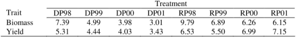
Table 4. Grain yield (kg ha-1) and biomass per plant (g) averaged over all 25 genotypes for rainfed (RP) and drought (DP) plots in period 1998-2001

Treatment

Trait DP98 DP99 DP00 DP01 RP98 RP99 RP00 RP01

Biomass 7.39 4.99 3.98 3.01 9.79 6.89 6.26 6.15

Yield 5.31 4.44 4.03 3.43 6.53 5.50 6.99 7.15

(10)

during vegetative growth, respectively. The explanation for relatively high soil moisture content in DP99 could be in a lot of precipitation during the spring time in 1999. It is expected that with more precipitation, there will be fewer sun hours, lower temperature, and thus, reduced evaporation. Moreover, since the first two PLS factors do not explain all the GEI for grain yield, some distortions occurred, e.g., treatments DP98 and DP99 are in same direction as sm covariables. The second cluster is in the lower left quadrant and includes RP99, RP01, and DP01. The year 2001 had a very low winter soil moisture reserve i.e. precipitation (Table 2) that caused the lowest mean grain yield in DP01 (Table 4). Both years (1999 and 2001) were rainy, with fewer sun hours and reduced maximum (soil and air) temperatures (Table 2). The third cluster involves RP00 and DP00. The year 2000 was warmer, sunnier and drier than the average (Table 2).

Concerning the genotypes, most of them showed a positive grain yield interaction with the same treatment as for biomass per plant. Nevertheless, more landraces had positive interaction with warm and dry 2000 for grain yield than for biomass. For example, landraces 17 and 21 had positive interaction with RP99 for biomass, but for grain yield they were favoured by conditions in DP00. Or, landraces 18 and 20 had positive biomass interaction with treatments in 2001, but for grain yield interacted better with treatments in 2000. This suggests that different plant trait(s) than biomass allows these landraces to achieve relatively better yield in warm and dry conditions. Tested cultivars had significantly higher grain yield than landraces and there was no one with positive interaction with 2000. This is expected since many wheat breeding programs in Serbia hadbeen carried out under non-limiting conditions. Cultivars 1, 2, 3, and 5 had positive yield interaction with treatments in 1998 and 1999 when a higher level of water in the soil was recorded. Nevertheless, the cultivar 4 exhibited a positive interaction with DP01 in which plants experienced water stress starting from tillering because of low wpp and high mT3 and smt3.

CONCLUSION

The PLS regression model was used to determine the most informative subset of environmental covariables affecting GEI for biomass per plant and grain yield in wheat. Results of this study indicated that mean maximum soil temperature in April and May, mean soil moisture in March, and mean sun hours per day in May were correlated to PLS factor that explained most of the GEI for biomass per plant. Similar results were obtained for grain yield. The environmental covariables that mostly explained GEI for this trait were mean maximum soil temperature in April and May, mean sun hours per day in May, and mean maximum soil temperature in June.

(11)

Generally, wheat landraces are able to better exploit warm and dry environments than cultivars. On the other hand cultivars are favoured by environments with higher soil moisture content during the vegetative growth (March to June). Having in mind global climate changes (decrease in annual precipitation and an increase in mean annual temperatures) it seems that some of the tested landraces could be regarded as useful for improving yield of new varieties for regional markets.

Received Septembert 29th_{, 2007}

Accepted November 5th_{, 2007}

REFERENCES

AASTVEIT, H. and H. MARTENS (1986): ANOVA interactions interpreted by partial least squares

regression. Biometrics, 42, 829-844.

ANNICCHIARICO, P. (1997): Additive main effects and multiplicative interaction (AMMI) analysis of

genotype-location interaction in variety trials repeated over years. Theor. Appl. Genet., 94, 1072-1077.

BLUM, A. (1988): Plant breeding for stress environments. CRC Press, Boca Raton, FL.

CROSSA, J. (1990): Statistical analyses of multilocation trials. Adv. Agron., 45, 55-85.

DODIG, D. (2005): Ocena genotipova pšenice prema suši. Doktorska disertacija, Univerzitet u Beogradu, Poljoprivredni fakultet–Zemun.

GABRIEL, K.R. (1971): The biplot graphic display of matrices with application to principal component

analysis. Biometrika, 58, 453–467

KAYA, Y., M. AKCURA, R. AYRANCI and S. TANER (2006): Pattern analysis of multi-environments trials in bread wheat. Commun. Biometry Crop Sci., 1, 63-71.

KROONENBERG, P.M. (1995): Introduction to biplots for G × E tables. Department of Mathematics,

Research Report 51, University of Queensland, AUS.

LILLEMO, M., M. van GINKEL, R.M. TRETHOWAN, E. HERNANDEZ and S. RAJARAM (2004):

Associations among international CIMMYT bread wheat yield testing locations in high rainfall areas and their implications for wheat breeding. Crop Sci., 44, 1163-1169.

QUARRIE, S.A., J. STOJANOVIC and S. PEKIC (1999): Improving drought resistance in small grained

cereals: a case study, progress and prospects. Plant Growth Regul. 29, 1-21.

REYNOLDS, M.P., K.D. SAYRE and S. RAJARAM (1999): Physiological and genetic changes of irrigated

wheat in the post green revolution period and approaches for meeting projected global demand. Crop Sci., 39, 1611-1621.

StatSoft Inc. (2004): STATISTICA (data analysis software system), version 7.1 (http://www.statsoft.com).

SHEARMAN, V.J., R. SYLVESTER–BRADLEY, R.K. SCOTT and M.J. FOULKES (2005): Physiological

processes associated with wheat yield progress in the UK. Crop Sci., 45, 175-178.

TALBOT, M. and A.V. WHEELWRIGHT (1989): The analysis of genotype × environment interactions by

(12)

VARGAS, M., J. CROSSA, F. van EEUWIJK, K.D. SAYRE and M.P. REYNOLDS (2001): Interpreting treatment × environment interaction in agronomy trials. Agron. J., 93, 949-960.

van GINKEL, M., D.S. CALHOUN, S. GEBEYEHU, A. MIRANDA, C. TIAN-YOU, R. PARGAS LARA, R.M.

TRETHOWAN, K. SAYRE, J. CROSSA and S. RAJARAM (1998): Plant traits related to yield of

wheat in early, late, or continuous drought conditions. Euphytica, 100, 109-121.

VARGAS M., J. CROSSA, K. SAYRE, M. REYNOLDS, M.E. RAMIREZ and M. TALBOT (1998): Interpreting

genotype × environment interaction in wheat using partial least squares regression. Crop Sci., 38, 679–689.

VARGAS M., J. CROSSA, F.A. van EEUWIJK M.E. RAMIREZ and K. SAYRE (1999): Using partial least

square regression, factorial regression, and AMMI models for interpreting genotype × environment interaction. Crop Sci., 39, 955-967.

WAGGONER, P.E. (1993): Preparing for climate change. In International Crop Science I. Crop Science

(13)

ANALIZA OGLEDA SA GENOTIPOVIMA PŠENICE KORIŠ ENJEM FAKTORA SREDINE

Dejan DODIG1_{, Miroslav ZORI} 2_{, Desimir KNEŽEVI} 3_{, Bojana}

DIMITRIJEVI 2_{i Gordana ŠURLAN-MOMIROVI} 2

1

Institut za kukuruz, Zemun Polje“, Beograd

2 _{Institut za ratarstvo, Poljoprivredni fakultet, Beograd} 3 _{Poljoprivredni fakultet, Univerzitet u Prištini, Zubin Potok}

I z v o d

U cilju utvr ivanja klimatskih i zemljišnih faktora kojima se najbolje može objasniti interakcija biomase i prinosa genotipova pšenice sa spoljašnjom sredinom primenjen je model regresije parcijlnih najmanjih kvadrata (PLS). Koriš en je set podataka iz ogleda sa 20 lokalnih populacija i 5 priznatih doma ih sorti pšenice. Genotipovi pšenice su tokom etiri godine (1998-2001) ispitivani u dva razli ita režima gajenja: prirodni uslovi i u uslovima suvog polja. Zaštitni krov iznad suvog polja svake godine je postavljen na kraju zimskog perioda (po etkom marta), u fazi bokorenja biljaka.

Za oba anlizirana svojstva ANOVA je pokazala da je interakcija genotip × uslovi gajenja (tretman) visoko signifikantna (P<0.001). Rezultati PLS modela su pokazali da prva i druga dimezija (latentni faktori) objašnjavaju 31.9 i 12.5% interakcije genotipa sa spoljnom sredinom za biomasu po biljci, odnosno 31.2 i 18.4% za prinos zrna, respektivno. Faktori spoljašnje sredine kao što su maksimalna temperatura zemljišta na 5 cm dubine u aprilu i maju, vlažnost zemljišta u sloju od 75 cm u martu i trajanje dnevnog osun avanja u maju mesecu u najve oj meri doprinose interakciji genotipa sa uslovima gajenja za biomasu po biljci. Sli ni rezultati su dobijeni za prinos zrna, s tom razlikom da se umesto faktora vlažnost zemljišta u sloju od 75 cm u martu mesecu kao zna ajana pokazala temperatura zemljišta na 5 cm dubine u junu mesecu.

Generalno, lokalne populacije pšenice su ispoljile bolju prilago enost sredinama sa visokim temperaturama (vazdušnim i zemljišnim) i manjom dostupnoš u vode tokom vegetativnog perioda (mart-jun) od sorti pšenice.