www.geosci-model-dev.net/8/3715/2015/ doi:10.5194/gmd-8-3715-2015
© Author(s) 2015. CC Attribution 3.0 License.
The Explicit Wake Parametrisation V1.0: a wind farm
parametrisation in the mesoscale model WRF
P. J. H. Volker, J. Badger, A. N. Hahmann, and S. Ott
Wind Energy Department, Technical University of Denmark, Risø Campus, Roskilde, Denmark Correspondence to:P. J. H. Volker ([email protected])
Received: 15 April 2015 – Published in Geosci. Model Dev. Discuss.: 29 April 2015 Revised: 3 November 2015 – Accepted: 5 November 2015 – Published: 18 November 2015
Abstract.We describe the theoretical basis, implementation, and validation of a new parametrisation that accounts for the effect of large offshore wind farms on the atmosphere and can be used in mesoscale and large-scale atmospheric models. This new parametrisation, referred to as the Explicit Wake Parametrisation (EWP), uses classical wake theory to describe the unresolved wake expansion. The EWP scheme is validated for a neutral atmospheric boundary layer against filtered in situ measurements from two meteorological masts situated a few kilometres away from the Danish offshore wind farm Horns Rev I. The simulated velocity deficit in the wake of the wind farm compares well to that observed in the measurements, and the velocity profile is qualitatively simi-lar to that simulated with simi-large eddy simulation models and from wind tunnel studies. At the same time, the validation process highlights the challenges in verifying such models with real observations.
1 Introduction
Wind turbines capture the kinetic energy of the wind with their turning blades, which transfer the energy to a transmis-sion system that drives an electric generator. In this process the flow in front and behind a wind turbine is decelerated by the forces acting on the rotating blades. In large wind farms, the interaction of the flow and the wind turbines is further complicated by the interaction of the wake of one wind tur-bine with neighbouring turtur-bines. Besides the changed veloc-ity field around the turbines, there is also evidence that wind turbines affect planetary boundary layer (PBL) processes due to the changed turbulence (Baidya Roy et al., 2004; Calaf et al., 2010; Baidya Roy and Traiteur, 2010; Barrie and
Kirk-Davidoff, 2010; Wang and Prinn, 2010; Lu and Porté-Agel, 2011; Hasager et al., 2013; Fitch et al., 2013a).
Coastal regions are expected to become major areas for wind energy production, since winds there are generally strong, steady, and less turbulent. To obtain an optimal yield, which is, among other things, a function of power produc-tion, electrical cabling, and installation costs, it is often con-venient to group wind farms together. Examples are the Dan-ish Rødsand 2 and Nysted or the Belgian Belwind, North-wind, and Thornton wind farms, in which the wind farm sep-aration is only a few kilometres. In planning new wind farms near existing ones it is important to estimate the velocity per-turbation from the nearby farm as accurately as possible, be-cause the power production is highly sensitive to the wind speed. Velocity deficits behind wind farms can be consid-erable. Christiansen and Hasager (2005), for example, found for near-neutral atmospheric stability, velocity deficits of 2 % up to 20 km downstream of the Horns Rev I (25 km2) wind farm. The accurate measurement of wakes from nearby farms becomes even more important in light of the fact that as of 2015 large offshore wind farms cover areas of up to 100 km2. Mesoscale models are suitable tools to estimate wind energy resources in these sea areas (Hahmann et al., 2014). How-ever, the collective effect of the wind turbines to the flow needs to be included in these models, and because these oc-cur at scales smaller than the model’s grid size and remain unresolved, the effects have to be parametrised.
on the other hand, is on the order of kilometres and tens of metres in the horizontal and vertical direction, respectively. This means that the profile of the turbine-induced velocity deficit can be captured to some extent in the vertical direc-tion. However, the downstream development of the velocity remains completely unresolved for scales smaller than the grid size. The major challenge in the parametrisation is to account for the unresolved relevant processes in agreement with the flow equations of the model. In recent years, steady progress has been made in the parametrisation of the effect of wind farms in global and mesoscale models: from the repre-sentation of wind farms by an increased roughness length in Keith et al. (2004) and Frandsen et al. (2009), up to the more advanced drag approaches in Adams and Keith (2007), Bla-hak et al. (2010), Baidya Roy (2011), Jacobson and Archer (2012), Fitch et al. (2012), Fitch et al. (2013b), and Abkar and Porté-Agel (2015). Apart from a local drag force, an ad-ditional turbulence kinetic energy (TKE) source term is as-sumed in the schemes proposed by Adams and Keith (2007), Blahak et al. (2010), Fitch et al. (2012), and Abkar and Porté-Agel (2015).
In this article we develop a new approach, which is here-after referred to as the Explicit Wake Parametrisation (EWP). We define the TKE from random fluctuations around the ensemble-averaged velocity, instead of around the grid-cell-averaged velocity as done in the previous parametrisations. Therefore, to be consistent with the flow equations of the model, we apply a grid-cell-averaged drag force, and addi-tional TKE is only provided by the PBL scheme where there is an increased vertical shear in horizontal velocity compared to the free-stream velocity profile.
We implemented the EWP scheme in the open-source Weather Research and Forecast (WRF) model (Skamarock et al., 2008). The WRF model already includes a wind farm parametrisation option (Fitch et al., 2012), denoted as WRF-WF, which has been validated against wind farm measure-ments (Jiménez et al., 2014). We validated the WRF-WF and EWP parametrisations against long-term meteorological (met) mast measurements in the wake of an offshore wind farm. To our knowledge, measurements in the wake of a wind farm have not been used for the validation of a wind farm parametrisation model in previous literature.
In Sect. 2, we explain the theoretical basis of the EWP scheme and its implementation in the WRF model. Section 3 describes the measurements, whereas Sect. 4 introduces the WRF model setup and the configuration of the EWP and WRF-WF scheme. In Sect. 5 both wind farm parametrisa-tions are validated against the met mast measurements in the wake of the wind farm. A discussion of the results finalises the article in Sect. 6, followed by the conclusions in Sect. 7.
-2 -1 0 1
0 2 4 6
wind speed
distance
grid size
u
u u
u′′
u′
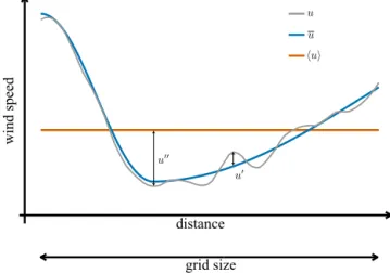
Figure 1.A sketch of the downstream development of a turbine-induced velocity reduction. Thexaxis indicates the grid-cell size. The grey line represents the instantaneous velocity and the coloured lines the averaged values. The difference between the average and instantaneous velocity defines the turbulence fluctuation at each dis-tance.
2 The Explicit Wake Parametrisation
We start by introducing the relevant mesoscale model equa-tions. Thereafter, the additional terms that represent the ef-fect of the wind turbines are derived and added to the model equations. At the end of the section their implementation in the mesoscale model is described.
2.1 The mesoscale model framework
Wind turbines are well described by drag devices that slow down the wind velocity from a free-stream valueu. Down-stream, due to mixing of fluid particles from within and out-side the wake, the velocity deficit is gradually reduced to the point at which the background conditions are restored.
We use a mesoscale model for the simulation of the wind farm wake and its recovery. It uses the Reynolds-averaged Navier–Stokes (RANS) equations,
∂ ui
∂ t +uj ∂ ui
∂ xj +
∂ u′ iu′j
∂ xj
= −1
ρ ∂ p ∂xi
−2εij kjuk−δi3g+fdi, (1) to describe the flow evolution. We use an overline to denote ensemble-averaged quantities and a prime for a fluctuation around the ensemble average. The exception is the average air densityρ(x, t ), where t denotes the time and x the
po-sition. In Eq. (1), ui(x, t ) and p(x, t ) represent the mean
velocity components and the pressure, whereas j and g
are the Earth’s rotation vector and the gravitational acceler-ation constant. Furthermore, the rightmost termfdi(x, t )is
Mesoscale models generally simulate the effects of turbu-lence in the vertical direction only. The components of the Reynolds stress are parametrised in a 1.5-order PBL scheme as
u′iu′3= −Km∂ ui ∂ x3
, (2)
where the turbulence diffusion coefficient for momentum, Km(x, t )=Smℓ
u′iu′i
1 2
, depends on the stability function Sm(x, t ), the turbulence length scale ℓ(x, t ), and the TKE
per unit mass,u′iu′i/2. We write the most general form of the TKE equation:
∂ e
∂t +T =ps+pb+pt−ǫ, (3) where on the left hand side (l.h.s.) edenotes the TKE and T the transport, which includes the advection by the mean flow, turbulence transport of TKE, and the divergence of the pressure correlation. On the right hand side (r.h.s.),ps rep-resents the turbulence production from the vertical shear in the horizontal velocity (shear production),pbthe turbulence production or destruction related to buoyancy forces,pt the turbulence induced by the turbine rotor, andǫthe dissipation. 2.2 The mesoscale model grid
For the mesoscale model, the previously defined variables in the Eqs. (1) and (3) have to be redefined on the three-dimensional model grid. For the parametrisation, we aim to obtain expressions for the volume-averaged drag force,
hfdi, and the volume-averaged turbulence induced by the turbine,hpti, that are consistent with the mesoscale model flow equations. Here, the angle brackets denote the volume average.
A new volume-averaged velocity equation is derived by integrating Eq. (1) over the grid-cell volume. This gives the expression forhfdi, which is derived in the following sec-tion (Sect. 2.2.1).
The derivation of the additional term hpti depends on the definition of the velocity perturbation. Formally, a veloc-ity perturbation is the difference between the instantaneous and ensemble-averaged velocity. For homogeneous flows, the spatially averaged velocity can be used for the defini-tion of a velocity fluctuadefini-tion, since the ensemble average can be approximated by the spatial average. However, the flow around wind turbines is non-homogeneous and conse-quently the spatial and ensemble average deviate. This has been illustrated in Fig. 1. Double averaging (ensemble and spatial) allows for the total kinetic energy to be separated into three components. The definition of the termhptiin the TKE equation will then depend on which of the three com-ponents contribute to the mean and which to the turbulence kinetic energy. In Appendix A, we discuss in more detail the double averaging and the ways mean and turbulence kinetic energy can be described.
In the EWP scheme, we follow Raupach and Shaw (1982) and Finnigan and Shaw (2008) and define a turbulence fluctu-ation around the ensemble mean (approach 1 in Appendix A). Therefore, we include only the random motion in the TKE.
With this definition, the additional term becomeshpti = hu′
i,hfd′ii, wherehis the hub height of the turbine. When we usefdi= −ρ Arctu
2
i,h/2 for the drag force, wherect(u) is the thrust coefficient andArthe rotor area, we obtain:
hpti = hui,hfdii − hui,hfdii
= −ρ Arcth(ui,h+u′i,h) u2i,hi/2+ρ Arcthui,hu2i,hi/2
≈ −ρ Arct
ui,hu′i2,h
. (4)
This term represents a sink of TKE due to the extraction of momentum. The magnitude of this term is much smaller than the additional term in the WRF-WF scheme (see Sect. 4.1.2). Therefore, the additional termhptiis neglected in the EWP approach. Additional turbulence is generated by shear pro-duction, which we assume to be the dominant mechanism on the grid-cell average.
In the following sections, we derive the expression for the grid-cell-averagedhfdi.
2.2.1 The sub-grid wake expansion
The velocity deficit expansion in the vertical direction within one grid cell is not negligible, which leads to flow decelera-tions that extend beyond the rotor-swept area. This part of the wake expansion is not accounted for in the mesoscale model, hence we estimate it explicitly with a sub-grid-scale (turbu-lence) diffusion equation. Then, a grid-cell-averaged force is determined and added to the model RANS equations.
In this model, we assume the horizontal advection of ve-locity and the turbulence diffusion to dominate in Eq. (1). Considering first only the flow behind the turbine rotor, we obtain the diffusion equation from Eqs. (1) and (2):
uo ∂
∂ x (uo−bu)=K ∂2
∂ z2 (uo−bu)+K ∂2
∂ y2 (uo−bu) , (5) which describes the expansion of the velocity deficit,uo−bu, behind the turbine. Here, uo= |u(h, t )| denotes the advec-tion velocity at hub height andbu(x)the unresolved veloc-ity in the stream-wise direction x in the wake of the tur-bine. The turbulence diffusion, which causes the wake ex-pansion, is described by a single turbulence diffusion coef-ficientK(x, y, t )=Km(x, y, h, t )in Eq. (2) and is given by the PBL scheme in WRF.
2.2.2 The velocity deficit profile
Equation (5) can be solved for the velocity deficit profile:
ud=usexp "
−1
2
z−h σ 2 −1 2 y σ 2# , (6)
where the length scale, σ, that determines the wake expan-sion is
σ2=2K
uo x+σ 2
o. (7)
Equation (6) describes the ensemble-averaged profile of the velocity deficit around hub height at a given point in the far wake (Tennekes and Lumley, 1972). Equation (7) rep-resents the vertical wake extension, resulting from turbulent diffusion of momentum, and it is similar to the solution of Eq. (4.29) in Wyngaard (2010) for the dispersion of plumes. Normally, the turbine wake is divided into a near and far wake, where the far wake begins between 1 and 3 rotor diam-eters (Vermeer et al., 2003; Crespo and Hernández, 1996). In the parametrisation, we account for the near-wake expansion in the initial length scaleσoand describe the unresolved far wake expansion with Eq. (6).
We can find the velocity deficit profile for wind turbines by equating the total thrust to the momentum removed by the action of the wind turbine, i.e.
1 2ρ ctπ r
2 ou2o=
∞ Z −∞ ∞ Z −∞
ρ uouddzdy=ρ uous2π σ2, (8)
whererois the radius of the rotor. In Eq. (8), the l.h.s. repre-sents the local forces at the rotor swept area, whereas the r.h.s. describes the equivalent distributed force for the ex-panded wake at any x. From the Eqs. (8) and (6), we find the velocity deficit profile for a specific thrust force,
ud= ctro2uo
4σ2 exp " −1 2 z −h σ 2 −1 2 y σ 2# . (9)
When we insert the velocity deficit of Eq. (9) in the second term of Eq. (8) and integrate in the cross-stream directiony, we have the integrated thrust profile
fd= ∞ Z −∞ ∞ Z −∞
ρ uouddzdy
= ∞ Z −∞ ρ r π 8
ctro2u2o σ exp
"
−1
2
z−h σ
2#
dz. (10)
The term on the r.h.s. within the integral describes the equiv-alent distributed thrust force in the vertical direction at any distancex. Next, we derive from Eq. (10) a single effective thrust force, which represents the average wake expansion within a grid cell.
2.2.3 Turbine forcing in the mesoscale model
For the mesoscale model we derive an effective thrust force, which describes the average wake expansion within a grid cell. Therefore, we first determine the effective velocity deficit profileueby averaging the velocity deficit of Eq. (9) over the cross-stream directionyand over a downstream dis-tance L that the wake travelled within the grid cell. It is convenient to approximate this area-averaged velocity deficit profile by a Gaussian-shaped profile:
ue= r
π 8
ctro2uo σe exp " −1 2
z−h σe 2# ∼ = 1 L L Z 0 ∞ Z −∞
uddydx.
(11) In Appendix B, we compare the area-averaged velocity deficit profile to the approximated Gaussian-shaped profile. In Eq. (11),σeis the effective length scale that is related to the model grid size,
σe= 1 L
L Z
0
σdx= uo
3K L "
2K uo L+σ
2 o
3 2
−σo3 #
. (12)
From the definition of the effective length scale, we can ob-tain the total effective thrust force fe by substituting the length scaleσ in Eq. (10) with the effective length scaleσe. This gives
fe= ∞ Z −∞ ρ r π 8
crro2u2o σe exp " −1 2 z −h σe 2# dz. (13)
The grid-cell-averaged acceleration for the model RANS equations, Eq. (1), is now obtained when we divide Eq. (13) by the mass and apply the grid-cell volume. For every verti-cal model layerk, we then obtain from Eq. (13) the grid-cell-averaged acceleration components,
hfd1(k)i = −
r π 8
ctro2u2o
1 x 1 y σe
exp "
−1
2
z−h σe
2#
cos[ϕ(k)]
(14) and
hfd2(k)i = −
r π 8
ctro2u2o
1 x 1 y σe
exp "
−1
2
z−h σe
2#
2.3 Implementation in the WRF model
We assume every turbine within a grid cell to be positioned at its centre and useL=1 x/2 in Eq. (12). In the numerical model, Eqs. (14) and (15) are added to the numerical approx-imation of Eq. (1). Furthermore, Eq. (12) is used to determine the effective length scale σeof the vertical wake extension.
At every time step the total thrust force within a grid cell is obtained from a superposition of the single turbine thrust forces.
To a first approximation, we use the grid-cell-averaged ve-locity at hub height,huo,hi, as the upstream velocityuofor
all turbines within the same grid cell (see Sect. 6). The tur-bulence diffusion coefficient for momentum,Kin Eq. (12), comes from the selected PBL scheme. The parametrisation, therefore, can be used with any PBL scheme. However, to be consistent with the assumptions used in the derivation of the wind farm parametrisation, a 1.5-order closure scheme with a turbulence shear production term is recommended. A prac-tical description of how to use the EWP scheme in the WRF model is given in the section “Code availability” at the end of the paper.
3 Wind farm and measurements
3.1 The Horns Rev I wind farm and met masts
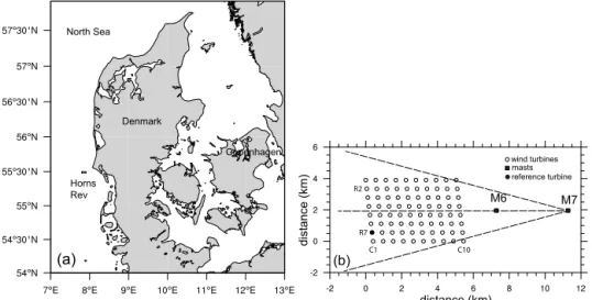
The parallelogram-shaped Horns Rev I wind farm is situ-ated in the North Sea about 15 km west of the Danish coast (Fig. 2). It is made up of 80 Vestas V80 (2 MW) pitch-controlled, variable-speed turbines, resulting in a total rated wind farm capacity of 160 MW. The turbines have a swept-area diameter of 80 m with the hub mounted at 70 m a.m.s.l. The equally spaced turbines are placed in 10 columns from west to east and 8 rows from north to south, labelled C1–C10 and R1–R8 in Fig. 2b. The spacing between columns and rows is 560 m, which is equivalent to 7 turbine diameters. Hansen et al. (2012) describe in detail the various produc-tion data available at the wind farm as well as their quality filtering and processing.
Turbine (C1, R7) is used as a reference turbine since it is not affected by the wind farm wake under westerly flows; in Fig. 2b it is marked with the solid bullet. The wind speed for each turbine is estimated from the power production data, using the turbine-specific power curve, and the wind direc-tion is obtained from the adjusted yaw angle (Hansen et al., 2012).
For the validation, we use data from two met masts, M6 and M7, whose positions are shown in Fig. 2b. The masts are located 2 and 6 km to the east of the eastern edge of the wind farm and are thus directly in its wake for westerly winds. The 70 m tall masts are identically equipped and their instrumen-tation includes high-quality Risø cup anemometers for mea-suring wind speeds. The 10 min averaged data from the two
masts, which are independent of the wind farm data, are used to validate the modelled wind speed reductions downstream from the wind farm.
3.2 Data selection and averaging for the validation For the validation of the results of the model simulations, and especially because of the relatively large area-averaged fields in the mesoscale model, it is very important to ensure that measurements and model fields are comparable. This can be achieved by properly selecting the wind direction and wind speed interval at the reference turbine.
Regarding the wind direction selection, for narrow wind direction sectors, Gaumond et al. (2013) found a higher mea-sured turbine production at Horns Rev I compared to that es-timated by wake models. Most likely this is related to wind direction variations, which, for small wind direction bins, ex-ceed the bin size within the 10 min averaging period. Since these variations are not accounted for in the model, we follow the recommendation of averaging over a relatively large wind direction interval. Furthermore, it is important that the flow reaching the mast anemometers has passed through the wind farm, as otherwise it does not characterise the wind farm wake. Therefore, we select velocities whose directions are at the reference turbine between 255 and 285◦. As demon-strated in Fig. 2b, the flow from this sector is influenced by the wind farm wake.
In the period 2005 to 2009, we select the 10 min aver-aged wind speeds from 6.5 to 11.5 m s−1at the reference tur-bine and bin them in 1 m s−1intervals. In this range, we are guaranteed to be above the cut-in wind speed of the turbines (4 m s−1) and below the wind speed at which the control sys-tem starts to pitch the blades (13 m s−1). To obtain as many data as possible, we do not filter the measurements on sta-bility. For strong westerly winds, we expect the atmospheric stability near to the ground on average to be neutral (Sathe et al., 2011).
For every instance that the wind direction and wind speed at the reference turbine was within the above-described range, the wind speeds at M6 and M7 were accepted. Af-terwards, the selected wind speeds were averaged for each wind speed bin and normalised by the average wind speed at the reference turbineuref(Table 1).
4 WRF model configuration and averaging
Horns Rev North Sea
Denmark
Copenhagen
(a)
M6 M7
wind turbines masts
C1 C10
R7 R2
distance (km)
distance (km)
(b)
reference turbine
Figure 2.Location(a)and layout(b)of the offshore wind farm Horns Rev I including two nearby masts (M6 and M7). The centre of the wind farm and width of the sector (±15◦) used for the filtering of the measurements are indicated by the dashed lines.
5∆x×5∆y
L40 L60 L80
0 2 4 6
z/z
h
(a) (b)
Figure 3. (a)Illustration of the model wind farm layout as applied in the mesoscale model. The squares indicate the model grid cells and the wind turbines are marked with triangles.(b)Height (normalised by the turbine hub height) of the model mass-levels for the three simulations: L40, L60, and L80. The solid grey line and the dashed lines mark the hub height and the upper and lower turbine blade tip, respectively.
Table 1.Average wind speed at the reference turbine (uref) and fre-quency of the measurements at the met mast for all wind speed bins within the wind direction range 255–285◦.
Wind speed bin uref Nobsat M6–M7 (m s−1) (m s−1)
7±0.5 7.00 887
8±0.5 7.95 933
9±0.5 8.95 1097
10±0.5 10.05 990
11±0.5 11.05 729
V80 turbines and extends over five grid cells in the west–east and north–south direction (Fig. 3a). The Vestas V80 thrust and power curves were used for the turbine parameters.
The model was run in an idealised case mode with open lateral boundary conditions (Skamarock et al., 2008, p. 51), Coriolis forcing, and zero heat fluxes from the lower bound-ary. At the surface, the no-slip condition holds. The to-tal domain is located over water, and we prescribe a con-stant roughness length of z0=2×10⁻⁴m, which follows the World Meteorological Organization (WMO) standards. The friction velocity is obtained with the Charnock formula. The model simulations were run with the MYNN 1.5-order level 2.5 PBL scheme (Nakanishi and Niino, 2009), on which the WRF-WF scheme is dependent. These and other details of the model configuration are summarised in Table 2.
Table 2.The WRF model configuration used in the simulations.
Number of grid cells in the horizontal plane (nx,ny): 80, 40
Horizontal grid spacing (km): 1.12
Domain size inx,y,z(km): 89.6, 33.6, 15 Wind farm extension (nx×ny): 5×5
Boundary condition: OPEN
PBL scheme: Nakanishi and Niino (2009)
Surface layer scheme: MYNN Monin–Obukhov similarity theory
TKE advection: Yes
Perturbation Coriolis: Yes
Roughness length (m): 2×10⁻⁴
Coriolis frequency (s−1) 1.2×10⁻⁴
Table 3.Details of the WRF simulations.
Wind direction range (◦): 258.75–281.25 Wind direction interval (◦): 3.75
Wind speeds (m s−1): 7.0, 8.0, 9.0, 10.0, and 11.0 Number of vertical levels (nz): 40 (L40), 60 (L60), 80 (L80) Wind farm parametrisation: None, WRF-WF, EWP
there are 5, 7, and 10 grid-cell volumes intersecting with the turbine rotor as shown in Fig. 3b.
All 135 simulations (5 wind speeds, 9 wind directions, and 3 vertical resolutions) were initialised with a constant geostrophic wind in height in a dry and slightly stable atmo-sphere. After a 4-day integration period, the wind converged in the whole domain to a logarithmic neutral profile within a 650 m deep boundary layer. The boundary layer was capped by an inversion layer with a potential temperature gradient of around 6 K km−1. Above the inversion layer the velocity re-mained independent of height. The atmospheric state of each of these 135 simulations was used to drive a control simula-tion without wind farm parametrisasimula-tion, a simulasimula-tion with the WRF-WF scheme, and a simulation with the EWP scheme. We used the restart option in the WRF model to initialise these simulations.
Each control or wind farm simulation lasted 1 day, result-ing in a total simulation length of 5 days. The wind speeds in the control simulations were 7, 8, 9, 10, and 11 m s−1at 70 m (hub height) after 5 days of simulation. We ended up with the desired magnitude of the geostrophic wind by con-ducting several experiments with different initialisations.
To summarise, we performed simulations for 9 wind di-rections, 5 wind speeds, and 3 vertical resolutions, with and without wind farm parametrisation, which gives a total of 405 (3 times 135) simulations as outlined in Table 3. For the validation against the mast measurements, we averaged the model wind speeds over the nine wind directions with a uniform direction distribution. We used the instantaneous wind speeds at the end of the simulation period for the val-idation. Like for the observations, we normalise the
wind-L80 L60 L40
1.9 R0
1.7 R0
1.5 R0 Turbine measurement
0.7 0.8 0.9 1.0
0 1000 2000 3000 4000 5000
Distance(m)
h
uh
i
/
h
uo,
h
i
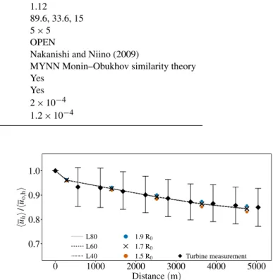
Figure 4.Measured and simulated hub-height velocity within the wind farm. The lines show the model-simulated velocities averaged over wind direction with an initial length scaleσo=1.7rofor the three vertical resolutions (L40, L60, and L80). The diamonds repre-sent the measured turbine velocity averaged over each row and the bars indicate their standard deviations. The crosses mark the veloc-ity at the grid-cell centre. The normalised velocveloc-ity forσo=1.5ro andσo=1.9rois shown with red and blue dots.
direction-averaged wind speeds and hereafter simply refer to them as “velocity”. The model wind speeds from the simula-tions without the wind farm were used to normalise the wind farm flow.
4.1 Wind farm parameters 4.1.1 The EWP scheme
We use the wind speeds, derived from the power production data of the turbines, to determine the initial length scaleσoin Eq. (12). To a first approximation, the initial length scale is defined to be independent of the upstream conditions, and it is therefore the same for all turbines. The initial length scale is assumed to scale with the rotor radius and accounts for the near-wake expansion.
a minimum of 850 observations for a turbine at the eastern edge of the wind farm and a maximum of 1612 observations for a turbine in the first wind farm column. The difference in the selected number of observations results from the ad-ditional requirement that, for a given turbine, the local up-stream turbines have to be operational in order to guarantee wake losses. For the power production data obtained in this way, we used the power curve to derive the wind speed. The column-averaged velocity was afterwards derived by averag-ing over the inner six rows (R2–R7). The outer rows were excluded because they experience different wake conditions under various wind directions.
Similarly to the model experiments in Sect. 4, we per-formed simulations for nine wind directions between 255 and 285◦for the three vertical resolutions with a wind speed at
hub height of 9 m s−1. To determine the best-fitting value, we varied for the EWP simulations the initial length scale for all turbines fromσo=ro toσo=2ro, stepping with1ro= 0.1. For the comparison to the measurements, the column-averaged wind speed was obtained by averaging over the 3 central wind farm grid cells in the cross-stream direction.
The lines in Fig. 4 show the hub-height velocity from the simulations with σo=1.7ro, which had the smallest over-all bias compared to the measurements. Additionover-ally, the coloured dots indicate the sensitivity to the initial length scale for σo=1.5 and 1.9ro. The figure shows the same veloc-ity reduction for all three vertical resolutions. Consequently, the amount of energy extracted by the turbines is indepen-dent of the vertical resolution. The simulations with an initial length scaleσo=1.7rofollow the measured velocity reduc-tion fairly well. We use this length scale for all simulareduc-tions in Sect. 5.
4.1.2 The WRF-WF scheme
In the validation, we also include results from the wind farm parametrisation WRF-WF from WRF-V3.6. This parametri-sation was introduced in WRFV3.3 by Fitch et al. (2012). In this approach, the grid-cell-averaged force, hfdi, is ap-proximated by the local forcing term at the turbine rotor. The scheme applies a fraction of the total drag force to ev-ery model level that intersects with the blade-sweep area of the wind turbine. Thus the scheme simulates the local drag forces over the turbine rotor. The additional TKE source term is parametrised as
hpt,WRF-WFi =ρ Ar(ct−cp)h |u| i3/2, (16) where cp is the power coefficient of the turbine andh |u| i the absolute value of the grid-cell velocity. The application of one-dimensional theory (Hansen, 2003) to Eq. (16) gives pt,WRF-WF=ρ Arctah |u| i3/2 for the additional TKE term. Here,adenotes the induction factor.
The same result,hpt,WRF-WFi =ρ Arctah |u| i3/2, is ob-tained by defining a velocity fluctuation as the difference
between the grid-cell-averaged velocity and the instanta-neous velocity (approach 2 in Appendix A). In Fig. 1, this velocity fluctuation has been denoted by u′′. An
an-alytical derivation can be found in Abkar and Porté-Agel (2015) (their Eq. 21, with theirξ=1). In this definition of TKE, the turbine-induced velocity reduction is counted as TKE. For the considered wind speeds, the absolute value of
hpt,WRF-WFiis around 30 times larger thanhptidefined in Eq. (4), which comes from the different definition of TKE in the two schemes. For example, for 10 m s−1withct=0.79, cp=0.43, andhu′i
2
,hi =0.7 m
2s−2 at hub height, the ratio betweenhpt,WRF-WFiandhptias has been defined in Eq. (4) is 32.
In Sect. 5, we use the updated WRF-WF parametrisation from WRFV3.6, which has no free parameters. The power and thrust coefficients come from the Vestas V80 turbine.
5 Validation of the wind farm parametrisations To obtain a complete picture of the modelled velocity field within and downstream of the Horns Rev I wind farm, we compare (1) the velocity decay in the wake of the wind farm from the two wind farm parametrisations to the measure-ments for the 10 m s−1wind speed bin, and (2) the modelled velocities to the measurements at M6 (2 km downstream) and M7 (6 km downstream) for all five wind speeds (7, 8, 9, 10, and 11 m s−1). We recall that the initial length scale used in the EWP scheme has been determined for 9 m s−1.
In a qualitative validation, we examine the velocity reduc-tion behind the wind farm and the profile of the velocity deficit. Furthermore, we discuss the vertical structure of the modelled TKE field from the discretised Eq. (3), where the additional termhptihas been parametrised in the WRF-WF scheme and neglected in the EWP scheme. We use results from independent LES simulations and wind tunnel experi-ments as a reference.
In the validation, we use the instantaneous model outputs from the converged flow field after the 5-day integration pe-riod. Furthermore, the velocities are normalised as described in the Sects. 3 and 4.
5.1 Velocity recovery at turbine hub height
Mast
M6
M7
L80 L60 L40 0.6
0.7 0.8 0.9 1.0
0 4000 8000 12000
Distance(m)
h
uh
i
/
h
uo,
h
i
Mast
M6
M7
L80 L60 L40 0.6
0.7 0.8 0.9 1.0
0 4000 8000 12000
Distance(m)
h
uh
i
/
h
uo
,
h
i
(a)
(b)
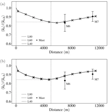
Figure 5.Hub-height velocity for the EWP(a)and WRF-WF(b)
parametrisations for the L40, L60, and L80 simulations and ob-servations as a function of distance from the western edge of the wind farm. The lines show the model simulated velocities, with the crosses showing the velocity at the grid-cell centre. The diamonds are used for the met mast measurements, and the bars are their stan-dard deviation. The vertical dashed lines show the wind farm ex-tension and the horizontal dotted line the velocity with the EWP scheme at the easternmost grid cell.
equilibrium has been reached within the wind farm between the extracted momentum by the wind turbines and the com-pensating flux of momentum from above. On the other hand, from the nearly constant velocity at the end of the wind farm for the WRF-WF scheme, it seems that the extraction of mentum by the turbines is almost balanced by the flux of mo-mentum from aloft. At the end of the wind farm the velocity difference between the two schemes is only 0.1 %. We have indicated the velocity from the EWP scheme at the most east-erly grid cell of the wind farm with a dotted horizontal line in Fig. 5. This agreement is noteworthy, given the two different methods used. At M6, 2 km downstream of the wind farm, the modelled velocity for both schemes is within the uncer-tainty of the measurements. Nevertheless, the difference be-tween the schemes is increased from 0.1 % at the end of the wind farm to 4.7 % at M6. This means that, downstream of the wind farm grid cells, where the wind farm parametrisa-tions are not active, the velocity diverges for the two schemes and its difference becomes significant. The near-wake recov-ery is important, especially if the velocity was used to esti-mate the power production on a neighbouring wind farm that was located at this distance from the original wind farm. For
example, the Rødsand 2 and Nysted offshore wind farms in southern Denmark are separated by a comparable distance.
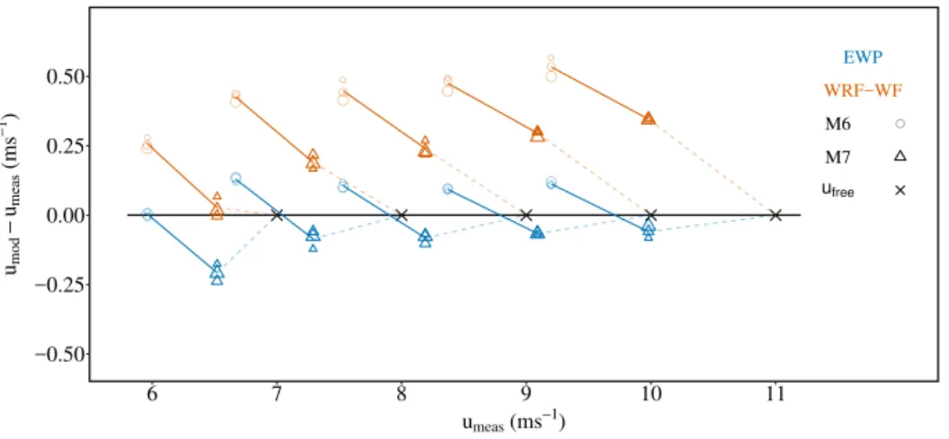
Figure 6 depicts wind-direction-averaged velocity recov-ery at the two met masts for all five wind speed bins and all vertical resolutions. It shows the differences in the WRF-modelled and measured wind speed at M6 (circles) and M7 (triangles) compared to the measured wind speed at the same masts. The WRF-modelled wind speed is obtained from lin-ear interpolation of the wind speeds in the nlin-earest grid cells. The modelled recovery rate can be deduced from the slopes of the solid (between the values at M6 and M7) and dashed lines (between M7 and the free-stream velocity). A negative slope is linked to a slower modelled recovery compared to that measured, whereas a positive slope shows a faster mod-elled recovery. There is no vertical resolution dependency for a wind farm parametrisation when the circles or triangles for a given wind speed bin lie on top of each other.
The results show that the bias in velocity between the mea-surements and the EWP simulations is small (<0.15 m s−1) for all wind speeds (except for the 7 m s−1bin at M7). For the EWP scheme, we find a positive velocity difference at M6 and a negative one at M7. Hence, the modelled wake re-covery oscillates between being slightly slower from M6 to M7 and being slightly faster from the end of the wind farm to M6, as well as from M7 to the end of the wake. The ve-locity of the EWP scheme at M6 is nearly independent of the vertical resolution, and at M7 the dependency is very weak.
The WRF-WF scheme shows a positive difference in ve-locity of up to 0.5 m s−1 at M6. This difference, between the WRF-WF scheme and the measurements, becomes larger with increasing wind speed. The higher modelled velocity at M6 is a consequence of the more rapid recovery of the mod-elled wake compared to that of the measurements from the end of the wind farm to M6. Between M6 and the point at which the free-stream velocity is reached again, the modelled wake recovery is slower than that measured. This overall positive difference suggests that the modelled velocity with the WRF-WF scheme is overestimated throughout the whole wake.
●
● ●
● ●
● ●
● ● ●
● ●
● ● ●
● ●
● ●
●
●
● ● ●
●
●
● ● ●
●
● EWP
WRF−WF
M6
M7
ufree
−0.50 −0.25 0.00 0.25 0.50
6 7 8 9 10 11
umeas (ms−1)
um
od
−
um
ea
s
(ms
−
1)
Figure 6.Modelled (umod) minus measured wind speeds (umeas) at M6 (circles) and M7 (triangles) as a function of their measured wind speed, for the EWP (blue symbols) and theWRF-WF scheme (red symbols) for five wind speed bins and three vertical resolutions (shown with different symbol sizes). The coloured solid lines link the M6 and M7 values for the same wind speed bin, whereas the dashed lines are the values from M7 and the free-stream velocities at the end of the wake. The crosses indicate the free-stream velocity.
0.80 0.85 0.90 0.95 1.00
-10 0 10
0.85
0.9
0.925
0.95 0.97 EWP L60
y
(
km
)
x(km)
0 10 20 30 40 50
0.80 0.85 0.90 0.95 1.00
-10 0 10
0.85
0.9
0.925
0.95 0.97
WRF-WF L60
y
(
km
)
x(km)
0 10 20 30 40 50
(a)
(b)
Figure 7.Horizontal view of the WRF-simulated velocity field at hub height using the(a)EWP and(b)WRF-WF schemes. The sim-ulations are for 10 m s−1in the 270◦wind direction and L60. The dotted line indicates the latitudinal centre and the solid rectangle the outer boundary of the wind farm.
Finally, Fig. 7 shows a difference in the orientation of the axis of the velocity deficit downstream from the wind farm. In both simulations the steady-state wind direction of the free-stream flow was 270◦. As the velocity decreases within the wind farm, the velocity is expected to turn to the north, due to the changed Coriolis force. In the wind farm wake, where the flow accelerates again, the velocity should turn back again to the background direction. This effect is seen
for the EWP scheme (Fig. 7a). However, for the WRF-WF scheme (Fig. 7b) the wake turns southward behind the wind farm. A possible reason for this unexpected behaviour is the turbulence transport of momentum from aloft (Ekman spiral) within the wind farm. In the wind farm wake the flow keeps turning to the south because of the flow acceleration from the momentum transport.
5.2 Vertical profile of TKE and velocity
To obtain a broader understanding of the mechanisms acting in the two schemes, we compare the simulated TKE (per unit mass) and the velocity deficit profiles for the 10 m s−1wind speed bin in the 270◦wind direction.
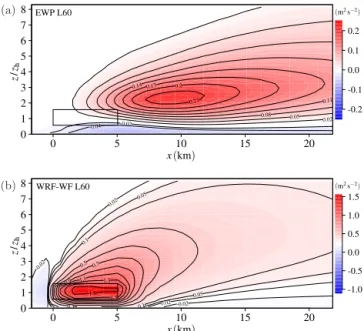
Figure 8 shows the difference in TKE (wind farm minus control simulation) for the L60 simulation. The cross sec-tions in thex–zplane are in the west–east direction and pass through the centre of the wind farm. We used different colour scales in the two plots, due to the relatively large differences in TKE production between the two schemes. However, we have kept the outermost contour (0.02 m2s−2) the same. The maximum TKE difference was 0.30 and 1.9 m2s−2 for the EWP and WRF-WF scheme, respectively.
-0.2 -0.1 0.0 0.1 0.2
0 1 2 3 4 5 6 7 8
-0.04 -0.02
0.02 0.05 0.08
0.11
0.140.17 0.2
0.23
EWP L60
z
/
zh
x(km)
(m2s−2)
0 5 10 15 20
-1.0 -0.5 0.0 0.5 1.0 1.5
0 1 2 3 4 5 6 7 8
-0.02
-0.02
0.02
0.02
0.05
0.05
0.1
0.1 0.3
0.50.7
0.9 1.1 1.3
1.5 1.8
WRF-WF L60
z
/
zh
x(km)
(m2s−2)
0 5 10 15 20
(a)
(b)
Figure 8. Vertical cross section of the TKE difference (hewfi − herefi) (m2s−2) for the simulations for 10 m s−1in the 270◦wind direction and L60 for the(a)EWP and(b)WRF-WF scheme. The region in the model containing turbine blades is indicated by the rectangle.
turbulence shear production (hpsi), we find that the inten-sity ofhptidominates over that of the shear production. The sum of the additional source term and the turbulence shear production causes within the wind farms an increased turbu-lence from the lowest model level upwards.
We use the results from the actuator-disc approach without rotation from Wu and Porté-Agel (2013) to obtain a qualita-tive impression of the structure of the turbulence field from an LES model within a wind farm. The actuator-disc ap-proach from their LES model is most similar to the drag approach in the mesoscale model. Their Fig. 5c shows that higher and lower turbulence intensities dominate around the upper and lower turbine blade tip. Also, a positive and neg-ative shear stress occur above and below hub height (their Fig. 7c). This indicates that the shear in velocity dominates the turbulence production. Similar features are present in the TKE field from the EWP scheme, where the increased and decreased TKE above and below hub height are, in a simi-lar manner, caused by an enhanced and reduced turbulence shear production with respect to the neutral logarithmic ve-locity profile. Furthermore, Wu and Porté-Agel (2013) show an upper wake edge at around 4.5 turbine hub heights for 10 aligned wind turbines after 60 turbine diameters (their Fig. 12). They defined the wake edge at the point where the velocity reduction for a given height was 1 %. Similarly, the edge of the wake can be found from an increased TKE due to shear production. For the outermost contour in Fig. 8, we obtain a vertical wake extension of around 5 turbine diame-ters for the EWP scheme at 4.8 km downstream (equivalent
to 60 turbine diameters). At the same distance, it is around 7 turbine hub heights for the WRF-WF scheme.
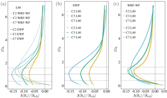
The influence of the TKE field to the velocity profile is analysed in Fig. 9. The figure shows the velocity deficit pro-file 1huxi/huo,hi for both schemes and all vertical
res-olutions. Here huo,hi denotes the free-stream velocity at
hub height. The velocity deficit is defined as 1hux(z)i = hu(z)i − hufree(z)i, wherehufree(z)iis the free-stream ve-locity profile from the reference simulation andhu(z)i the velocity profile from the wind farm simulation. The free-stream velocities from the EWP and WRF-WF simulations were visually indistinguishable. We choose the second and third grid cell within the wind farm (C2 and C3) and the sec-ond point behind the wind farm (C7) that correspsec-onds ap-proximately to the location of M6.
Figure 9a shows the velocity deficit profiles from the EWP and WRF-WF scheme from the L60 simulation. The profiles indicate a stronger diffusion in the WRF-WF scheme com-pared to that in the EWP scheme. This can be recognised by the vertical extension of the vertical deficit profile at C7, be-hind the wind farm.
For the EWP scheme (Fig. 9b), we find a maximum ve-locity deficit at hub height and symmetric features around the maximum for the L40 and L80 simulations. Also, re-sults from LES simulations, wind tunnel experiments, and measurements (Vermeer et al., 2003; Wu and Porté-Agel, 2013; Iungo et al., 2013) have a maximum velocity deficit at hub height in the far turbine wake for a neutral boundary layer. The profiles in Vermeer et al. (2003) (their Fig. 36) and in Wu and Porté-Agel (2013) (their Fig. 4) additionally show symmetric features around the maximum with a shape similar to the velocity profile of the EWP scheme. Fig-ure 9b demonstrates the vertical resolution independence of the EWP scheme within the wind farm: the velocity deficits of the L40 and L80 simulations are almost identical. A small difference is found below hub height in the wind farm wake. With the WRF-WF scheme (Fig. 9c) the maximum veloc-ity deficit is displaced vertically above hub height, which reaches the upper wind turbine blade tip at mast M6 (C7). The dependency of the WRF-WF scheme on the chosen ver-tical resolutions is weak; differences are found within the wind farm (C2, C3) above hub height. Also, the profiles from the WRF-WF scheme show increased (area-averaged) veloc-ities inside the wind farm at the lowest model level. The wind farm simulations from Wu and Porté-Agel (2013) (their Fig. 13) do not support this behaviour.
6 Discussion
L60
C2 WRF-WF
C3 WRF-WF
C7 WRF-WF
C2 EWP
C3 EWP
C7 EWP
0 2 4 6
-0.15 -0.10 -0.05 0.00
∆huxi/huo,hi
z
/
zh
EWP
C2 L80 C3 L80
C7 L80
C2 L40 C3 L40
C7 L40
0 2 4 6
-0.15 -0.10 -0.05 0.00
∆huxi/huo,hi
z
/
zh
WRF-WF
C2 L80
C3 L80
C7 L80
C2 L40
C3 L40
C7 L40
0 2 4 6
-0.15 -0.10 -0.05 0.00 0.05
∆huxi/huo,hi
z
/
zh
(a) (b) (c)
Figure 9.Comparison of the vertical profiles of simulated velocity deficit for the second (C2), third (C3), and seventh (C7) grid cell containing wind turbines from the first westernmost turbine:(a)L60 simulations,(b) L40 and L80 simulation for the EWP, and(c)L40 and L80 simulation for theWRF-WF scheme. The turbine hub height is indicated by the horizontal solid line and the turbine blade bottom and top by the dashed lines. The free-stream wind speed was 10 m s−1in the 270◦wind direction.
the proposed parametrisation, we use the classical wake the-ory (Tennekes and Lumley, 1972) to describe the sub-grid-scale wake expansion. Compared to empirical fits from, for example, Xie and Archer (2015) and Zang et al. (2013), it of-fers the advantage that the wake expansion is described as a function of atmospheric stability. In this study, we have vali-dated the approach for different wind speeds in a neutral at-mospheric boundary layer. Its performance as a function of atmospheric stability, which requires information of the pro-files, will be investigated in future. In their LES model re-sults, Wu and Porté-Agel (2013) found a sensitivity of the velocity reduction to the wind farm layout. In current imple-mentations of wind farm parametrisations, all turbines within a grid cell experience the same upstream velocity. Although these parametrisations are not meant to estimate the local ve-locity field within the wind farm, differences in veve-locity re-duction within the wind farm could affect the velocity in the wake of it. Future implementations may account for the local flow within the wind farm by using data from high-resolution models, which can be input to the mesoscale model via a look-up table as suggested by Badger et al. (2013) and Abkar and Porté-Agel (2015). However, we currently have no measurement data in the wind farm wake to validate these approaches for different wind farm layouts. At the Horns Rev I wind farm, we were restricted to the geometry of met masts positions, which did not allow for study of the sensitivity of the velocity field in the wind farm wake for additional wind direction sectors.
A fair comparison between the mesoscale model and long-term measurements can be realised in several ways. One
method is to match the simulation period to that observed. By selecting corresponding time frames, one can then com-pare the fields of interest. The main disadvantage of this method is that errors in the background flow simulated by the mesoscale model also exist, which complicates the anal-ysis. The second method is to sample the data and the model simulations in rather strict idealised conditions of wind speed and direction. We have chosen this second method using the WRF model in idealised case mode and compare its results to properly averaged measurements. Here the equilibrium so-lution without the wind farm effects is purposely made to match the free-stream velocity, and thus background errors in the simulations are absent. Besides a more detailed analy-sis, this method also allows for the study of the vertical de-pendency of the velocity reductions, since the atmospheric background conditions are almost identical for the simula-tions with different vertical resolusimula-tions.
validation of all wind speed bins. On the other hand, for the WRF-WF scheme we have used the turbine-specific thrust and power curves, which are its only input parameters. The difference of 0.1 % between the velocity deficit simulated by the WRF-WF and EWP scheme at the end of the wind farm for the 10 m s−1wind speed bin facilitated the compar-ison between the schemes in the wind farm wake, where the parametrisations are not active anymore.
One major difference between the EWP and WRF-WF approach is in the treatment of the grid-cell-averaged TKE budget equation. The TKE production regulates the verti-cal profiles of momentum, temperature, and moisture within the PBL. Differences in TKE production would thus affect the local weather (e.g. temperature, humidity, and possibly clouds) response to the presence of large wind farms. Both wind farm schemes use a PBL scheme that parametrises the TKE equation in terms of grid-cell-averaged variables. Therefore, in the wake of the wind turbines TKE is gener-ated by the increased vertical shear in horizontal velocity. Then, the different definition of the unresolved velocity fluc-tuation in the WRF-WF and EWP scheme leads to a differ-ent termhptithat is the direct consequence of the presence of a drag force. In the EWP scheme, a velocity fluctuation is defined around the ensemble-averaged velocity. With this definitionhptiis small and can be neglected. Instead, in the WRF-WF scheme, velocity fluctuations are defined around the grid-cell-averaged velocity and a parametrisation ofhpti
is added to the model TKE equation. The simulations have shown that, in the WRF-WF scheme,hpti dominates over the shear production and that its total TKE is more than 3 times larger than that in the EWP scheme. However, it is un-clear how well the actual grid-cell-averaged shear produc-tion is approximated by the shear producproduc-tion calculated with the PBL scheme in WRF, on which the EWP scheme re-lies. Therefore, future measurement campaigns of the actual structure and intensity of the TKE field within and around wind farms under suitable atmospheric conditions can help to settle this issue.
7 Conclusions
We introduce a wind farm parametrisation for use in mesoscale models. The EWP approach is based on classical wake theory and parametrises the unresolved expansion of
the turbine-induced wake explicitly in the grid cell that con-tains turbines, where the largest velocity gradients occur. The associated turbulence shear production is then determined by the PBL scheme in the mesoscale model. The approach has been implemented in the WRF mesoscale model and can be used with any PBL scheme. However, we recommend PBL schemes that model the TKE equation.
We analysed the results of simulations from the scheme in the wake of a wind farm. For the validation, we used the averaged wind speeds within a 30◦ wind direction sec-tor at two met masts in the wake of the Horns Rev I wind farm. The model was run for several wind direction bins that cover those sampled in the observations. For each wind speed bin, we compared a wind-direction-averaged wind speed to the similarly averaged measurements. We found that, for all five velocity bins, the velocity modelled with the EWP scheme agreed well with the met mast measurements 2 and 6 km downstream from the edge of the wind farm. The EWP scheme reproduces the wind farm wake within the standard deviation of the measurements.
Appendix A
We use the notation and symbols of Raupach and Shaw (1982), with the exception that the ensemble average is used
instead of the time average. The instantaneous velocity, ui,
can be decomposed in a spatial average with a fluctuation
around it,ui= huii +u′′i, and an ensemble average with a
fluctuation, ui =ui+u′i. Figure 1 illustrates the
instanta-neous velocity (grey line), as well as the spatial (red line) and ensemble-averaged (blue line) velocity in the vicinity of a wake.
We can decompose the total kinetic energy: 1
2
u2i=1
2
ui2+1
2
u′i2, (A1)
=1
2
ui 2
+1
2
u′′i2+1
2
u′i2. (A2) In Eq. (A1), we applied an ensemble and spatial averaging to the kinetic energy and we have decomposed the ensemble-averaged kinetic energy in an average and fluctuating part. Here,12hui2iis the spatial average of the ensemble-averaged
kinetic energy and 12hu′i2ithe spatial average of the kinetic energy from random velocity fluctuations.
By decomposing the first term on the r.h.s. of Eq. (A1), we obtain Eq. (A2). In Eq. (A2), we now have three con-tributions to the total spatial and ensemble-averaged kinetic energy. The first term, 12huii2, is the kinetic energy of the
spatial and ensemble-averaged velocity. The second term, 1
2hu
′′ i
2
i, is the spatially averaged kinetic energy of the het-erogeneous part of the mean flow, which is the difference between the ensemble and spatially averaged kinetic energy. This term arises only in non-homogeneous flow conditions and is also called “dispersive kinetic energy” by Raupach and Shaw (1982).
For each contribution on the r.h.s. of Eq. (A2) to the total kinetic energy, a budget equation can be derived. The com-plete set of equations can be found in, for example, Raupach and Shaw (1982). We can combine the three components in Eq. (A2) with kinetic energy of the mean flow (MKE) and turbulence kinetic energy (TKE) in two ways, which we refer to as approach 1 and 2. The MKE is not directly resolved by the model. However, the definition of TKE determines how the effect of wind turbines to the TKE is parametrised.
Approach 1 follows Raupach and Shaw (1982) and Finni-gan and Shaw (2008) and defines MKE =12hu2i i =12huii2+
1 2hu
′′ i
2
i and TKE = 12hu′i2i. Here, the MKE is equal to the spatial average of the ensemble-averaged kinetic energy, and it contains all kinetic energy of the organised motion. With this definition only random motion contributes to the TKE. The presence of the drag force gives rise to the term
hpti = hu′
ifd′ii, wheref
′is the fluctuation of the drag force
around the ensemble-averaged force. This approach is used in the EWP scheme, and in Sect. 2.2 the additional term is derived.
Approach 2 is the second way the three components in Eq. (A2) can be assigned to the MKE and TKE, namely MKE =12huii2and TKE =12hu′′i
2
i+12hu′i2i. In this case, the MKE contains only kinetic energy from the spatially averaged ve-locity. However, the TKE now also contains energy from the heterogeneous part of the mean flow additional to the energy from random motion. In this approach, a fluctuation can be decomposed inu′′=u′′i+u′i. Therefore, the source term be-comes hpti = hu′′i fd′′
ii, where f
′′ is the fluctuation of the
Appendix B
In the EWP scheme, we approximate the velocity deficit
pro-files on the r.h.s. of Eq. (11) by a Gaussian-shaped velocity profile on the l.h.s. of Eq. (11).
To show that these profiles are to a good approxima-tion similar, we compare the difference between the aver-age of 5000 single profiles at distances 0< x <500 m to the approximated Gaussian velocity deficit. We normalise both profiles by the depth, 1y, of the wake in the cross-stream direction. For the comparison we useduo=8 m s−1, ro=40 m, σo=60 m, cT=0.8, K=6 m2s−1, and 1 y=
1120 m. The wake centre is defined atz=0 m.
<Gaussian>
<Dispersion>
-200 -100 100 200
0.05 0.10 0.15
DUHmsL
zHmL
<G-D>
-200 -100 100 200
zHmL
-0.002
-0.001
0.001 0.002
DUHmsL
(a) (b)
Figure B1.Panel(a)shows a comparison between the distance average of the velocity deficit profiles (blue line) and the Gaussian profile with the average spreadhσi(red line). Panel(b)shows the difference between the spatially averaged Gaussian profiles and the Gaussian profile with the average spread.
Code availability
In this section a short guideline of the usage of the EWP scheme in the WRF model is given. The EWP approach can
be run in serial,shared-memory, or distributed memory
op-tions. Currently, it is not possible to run the approach with the mixed shared and distributed memory option. The scheme can be used for idealisedandreal case simulations. For the realcase simulations, the wind farm parametrisa-tion can be activated in any nest of the simulaparametrisa-tions. The ad-ditional namelist.input optionbl_turbineshould be used to select the wind farm parametrisation.
The EWP scheme needs additional input files in ASCII format. In the first file the positions and types of all wind turbines should be listed. The file name has to be spec-ified as a string in the additional namelist.input option
windturbines_spec. For every turbine used, the turbine
characteristics, i.e. the hub height and diameter and the thrust and power coefficients as a function of wind speed, need to be listed in a file. The power coefficient is used optionally to estimate the turbine power production. This file name has to start with the turbine type used in the first file, followed by the extension.turbine.
Please contact [email protected] to obtain the code of the EWP wind farm parametrisation.
The Supplement related to this article is available online at doi:10.5281/zenodo.33435.
Acknowledgements. Funding for research was provided through the European Union’s Seventh Programme, under grant agreement no. FP7-PEOPLE-ITN-2008/no238576 and no. FP7-ENERGY-2011-1/no282797. The authors gratefully acknowledge the suggestions and helpful discussions with Jerry H.-Y. Huang and Scott Capps, both from the Department of Atmospheric and Oceanic Sciences, UCLA. We would like to acknowledge Vattenfall AB and DONG Energy A/S for providing us with data from the Horns Rev I offshore wind farm and Kurt S. Hansen for the data processing and filtering. Finally, the authors want to thank the reviewers for their helpfull comments.
Edited by: S. Unterstrasser
References
Abkar, M. and Porté-Agel, F.: A new wind-farm parameterization for large-scale atmospheric models, J. Renewable Sustainable Energy, 7, 013121, doi:10.1063/1.4907600, 2015.
Adams, A. S. and Keith. D. W.: A wind farm parametrization for WRF, 8th WRF Users Workshop, 11–15 June 2007, Boulder, abstract 5.5, available at: http://www2.mmm.ucar.edu/wrf/users/ workshops/WS2007/abstracts/5-5_Adams.pdf, 2007.
Badger, J., Volker, P. J. H., Prospathospoulos, J., Sieros, G., Ott, S., Rethore, P.-E., Hahmann, A. N., and Hasager, C. B.:
Wake modelling combining mesoscale and microscale mod-elsm, in: Proceedings of ICOWES, Technical University of Denmark, 17–19 June 2013, Lyngby, p. 182–193, available at: http://indico.conferences.dtu.dk/getFile.py/access?resId= 0&materialId=paper&confId=126, 2013.
Baidya Roy, S.: Simulating impacts of wind farms on local hydrom-eteorology, J. Wind Eng. Ind. Aerod., 99, 491–498, 2011. Baidya Roy, S. and Traiteur, J. J.: Impact of wind farms on
sur-face air temperature, P. Natl. Acad. Sci. USA, 107, 17899–17904, 2010.
Baidya Roy, S., Pacala, S. W., and Walko, R. L.: Can large wind farms affect local meteorology?, J. Geophys. Res., 109, 2156– 2202, 2004.
Barrie, D. B. and Kirk-Davidoff, D. B.: Weather response to a large wind turbine array, Atmos. Chem. Phys., 10, 769–775, doi:10.5194/acp-10-769-2010, 2010.
Blahak, U., Goretzki, B., and Meis, J.: A simple parametrisa-tion of drag forces induced by large wind farms for numeri-cal weather prediction models, EWEC Conference, 20–23 April 2010, Warsaw, p. 186–189, available at: http://proceedings.ewea. org/ewec2010/allfiles2/757_EWEC2010presentation.pdf, 2010. Calaf, M., Meneveau, C., Meyers, J.: Large eddy simulation study
of fully developed wind-turbine array boundary layers, Phys. Fluids, 22, 015110, doi:10.1063/1.3291077, 2010.
Christiansen, M. B. and Hasager, C. B.: Wake effects of large off-shore wind farms identified from satellite SAR, Remote Sens. Environ., 98, 251–268, 2005.
Crespo, A. and Hernández, J.: Turbulence characteristics in wind-turbine wakes, J. Wind. Eng. Ind. Aerod., 61, 71–85, 1996. Finnigan, J. J. and Shaw, R. H.: Double-averaging methodology and
its application to turbulent flow in and above vegetation canopies, Acta Geophys., 56, 534–561, doi:10.2478/s11600-008-0034-x, 2008.
Fitch, A. C., Olson, J. B., Lundquist, J. K., Dudhia, J., Gupta, A., Michalakes, J., and Barstad, I.: Local and mesoscale impacts of wind farms as parameterized in a mesoscale NWP model, Mon. Weather Rev., 140, 3017–3038, 2012.
Fitch, A. C., Lundquist, J. K., and Olson, J. B.: Mesoscale influ-ences of wind farms throughout a diurnal cycle, Mon. Weather Rev., 141, 2173–2198, 2013a.
Fitch, A. C., Olson, J. B., and Lundquist, J. K.: Parameterization of Wind Farms in Climate Models, J. Climate, 26, 6439–6458, doi:10.1175/JCLI-D-12-00376.1, 2013b.
Frandsen, S. T., Jørgensen, H. E., Barthelmie, R., Badger, J., Hansen, K. S., Ott, S., Rethore, P.-E., Larsen, S. E., and Jensen, L. E.: The making of a second-generation wind farm ef-ficiency model complex, Wind Energy, 12, 445–458, 2009. Gaumond, M., Réthoré, P.-E., Ott, S., Peña A., Bechmann, A., and
Hansen, K. S.: Evaluation of the wind direction uncertainty and its impact on wake modeling at the Horns Rev offshore wind farm, Wind Energy, 7, 1169–1178, 2014.
Hahmann, A. N., Vincent, C. L., Peña, A., Lange, J., and Hasager, C. B.: Wind climate estimation using WRF model out-put: method and model sensitivities over the sea, Int. J. Climatol., 35, 3422–3439, doi:10.1002/joc.4217, 2014.
Hansen, M. O. L.: Aerodynamics of Wind Turbines, James & James, London, UK, 2003.
Hasager, C. B., Rasmussen, L., Peña, A., Jensen, L. E., and Réthoré, P.-E.: Wind farm wake: the Horns Rev Photo Case, En-ergies, 6, 696–716, 2013.
Iungo, G. V., Wu, Y.-T., and Porté-Agel, F.: Field measurements of wind turbine wakes with lidars, J. Atmos. Ocean. Tech., 30, 274– 287, 2013.
Jacobson, M. Z. and Archer, C. L.: Saturation wind power potential and its implications for wind energy, P. Natl. Acad. Sci. USA, 109, 15679–15684, 2012.
Jiménez, P. A., Navarro, J., Palomares, A. M., and Dudhia, J.: Mesoscale modeling of offshore wind turbine wakes at the wind farm resolving scale: a composite-based analysis with the Weather Research and Forecasting model over Horns Rev, Wind Energy, 18, 559–566, 2014.
Keith, D. W., DeCarolis, J. F., Denkenberger, D. C., Lenschow, D. H., Malyshev, S. L., Pacala, S., and Rasch, P. J.: The influence of large-scale wind power on global climate, P. Natl. Acad. Sci. USA, 101, 16115–16120, 2004.
Lu, H. and Porté-Agel, F.: Large-eddy simulation of a very large wind farm in a stable atmospheric boundary layer, Phys. Fluids, 23, 065101, doi:10.1063/1.3589857, 2011.
Nakanishi, M. and Niino, H.: Development of an improved turbu-lence closure model for the atmospheric boundary layer, J. Me-teorol. Soc. Jpn., 87, 895–912, 2009.
Porté-Agel, F., Wu, Y.-T., Lu, H., and Conzemius, R. J.: Large-eddy simulation of atmospheric boundary layer flow through wind tur-bines and wind farms, J. Wind Eng. Ind. Aerod., 99, 154–168, 2011.
Raupach, M. R. and Shaw, R. H.: Averaging procedures for flow within vegetation canopies, Bound.-Lay. Meteorol., 22, 79–90, doi:10.1007/BF00128057, 1982.
Sathe, A., Gryning, S.-E., and Peña, A.: Comparison of the atmo-spheric stability and wind profiles at two wind farm sites over a long marine fetch in the North Sea, Wind Energy, 14, 767–780, 2011.
Skamarock, W., Klemp, J., Dudhia, J., Gill, D., Barker, D., Duda, M., Huang, X., Wang, W., and Powers, J.: A Description of the Advanced Research WRF Version 3, NCAR Technical note, Massachusetts, USA, 2008.
Tennekes, H. and Lumley, J. L.: A First Course in Turbulence, The MIT Pess, Boulder, USA, available at: http://www2.mmm.ucar. edu/wrf/users/docs/arw_v3.pdf, 1972.
Vermeer, L. J., Søensen, J. N., and Crespo, A.: Wind turbine wake aerodynamics, Prog. Aerosp. Sci., 39, 467–510, 2003.
Wang, C. and Prinn, R. G.: Potential climatic impacts and reliability of very large-scale wind farms, Atmos. Chem. Phys., 10, 2053– 2061, doi:10.5194/acp-10-2053-2010, 2010.
Wu, Y.-T. and Porté-Agel, F.: Simulation of turbulent flow in-side and above wind farms: model validation and layout effects, Bound.-Lay. Meteorol., 146, 181–205, 2013.
Wyngaard, J. C.: Turbulence in the Atmosphere, Cambridge Press, Cambridge, UK, 2010.
Xie, S. and Archer, C.: Self-similarity and turbulence characteristics of wind turbine wakes via large-eddy simulation, Wind Energy, 18, 1815–1838, doi:10.1002/we.1792, 2015.