NeuralNetwork Based 3D Surface Reconstruction
Vincy Joseph
Computer Department
Thadomal Shahani Engineering College, Bandra, Mumbai, India.
Shalini Bhatia
Computer Department
Thadomal Shahani Engineering College, Bandra, Mumbai, India.
Abstract—This paper proposes a novel neural-network-based adaptive hybrid-reflectance three-dimensional (3-D) surface reconstruction model. The neural network combines the diffuse and specular components into a hybrid model. The proposed model considers the characteristics of each point and the variant albedo to prevent the reconstructed surface from being distorted. The neural network inputs are the pixel values of the two-dimensional images to be reconstructed. The normal vectors of the surface can then be obtained from the output of the neural network after supervised learning, where the illuminant direction does not have to be known in advance. Finally, the obtained normal vectors can be applied to integration method when reconstructing 3-D objects. Facial images were used for training in the proposed approach
Keywords-Lambertian Model;neural network;Refectance Model; shape from shading surface normal and integration
I. INTRODUCTION
Shape recovery is a classical computer vision problem. The objective of shape recovery is to obtain a three-dimensional (3-D) scene description from one or more two-dimensional (2-D) images. Shape recovery from shading (SFS) is a computer vision approach, which reconstructs 3-D shape of an object from its shading variation in 2-D images. When a point light source illuminates an object, they appear with different brightness, since the normal vectors corresponding to different parts of the object’s surface are different. The spatial variation of brightness, referred to as shading, is used to estimate the orientation of surface and then calculate the depth map of the object
II. DIFFERENT APPROACHES FOR RECONSTRUCTION
A. Lambertain Model
A successful reflectance model for surface reconstructions of objects should combine both diffuse and specular components [1]. The Lambertian model describes the relationship between surface normal and light source direction by assuming that the surface reflection is due diffuse reflection only. This model ignores specular component.
B. Hybrid Reflectance Model
A novel hybrid approach generalizes the reflectance model by considering both diffuse component and specular component. This model does not require the viewing direction and the light
source direction and yields better shape recovery than previous approaches.
A hybrid approach uses two self-learning neural networks to generalize the reflectance model by modeling the pure Lambertian surface and the specular component of the non-Lambertian surface, respectively. However, the hybrid approach still has two drawbacks:
1) The albedo of the surface is disregarded or regarded as constant, distorting the recovered shape.
2) The combination ratio between diffuse and specular components is regarded as constant, which is determined by trial and error.
C. Neural Network Based Hybrid Reflectance Model
This model intelligently integrates both reflection components. The pure diffuse and specular reflection components are both formed by similar feed-forward neural network structures. A supervised learning algorithm is applied to produce the normal vectors of the surface for reconstruction. The proposed approach estimates the illuminant direction, viewing direction, and normal vectors of object surfaces for reconstruction after training. The 3-D surface can also be reconstructed using integration methods.
III. DESCRIPTION
Fig. 1 shows the schematic block diagram of the proposed adaptive hybrid-reflectance model, which consists of the diffuse and specular components. This diagram is used to describe the characteristics of diffuse and specular components of adaptive hybrid-reflectance model by two neural networks with similar structures. The composite intensity Rhybrid is obtained by combining diffuse intensity Rd
and the specular intensity Rs based on the adaptive weights
λd(x,y) and λs(x,y) . The system inputs are the 2-D image
intensities of each point, and the outputs are the learned reflectance map.
Figure 1 Block diagram of the proposed adaptive hybrid-reflectance model
Figure 2 Framework of the proposed symmetric neural network for diffuse reflection model
The light source direction and the normal vector from the input 2-D images in the left side of the symmetric neural network are separated and then combined inversely to generate the reflectance map for diffuse reflection in the right side of the network. The function of each layer is discussed in detail below.
A. Function of Layers
Layer 1: This layer normalizes the intensity values of the input images. Node Ii denotes the ith pixel of the 2-D image and m
denotes the number of total pixels of the image. That is
,
i i
I
f
=
i
=
1
,....,
m
,
) 1 (
i
i
f
a
=
i
=
1
,....,
m
(1) Layer 2: This layer adjusts the intensity of the input 2-D image with corresponding albedo value.,
i i i
I f
α
=
i
=
1
,....,
m
Layer 3: The purpose of Layer 3 is to separate the light source direction from the 2-D image. The light source directions of this layer are not normalized.
,
ˆ
,
1
j i d m
i i
j
I
f
∑
ω
=
=
i
=
1
,...,
m
j
=
1
,
2
,
3
(3),
) 3 (
j j
j
a
f
s
′
=
=
j
=
1
,
2
,
3
2 3 2 2 2 1
1
s
s
s
f
j′
+
′
+
′
=
j
=
1
,
2
,
3
(4)2 3 2 2 2 1 ) 4 (
.
s
s
s
s
s
f
a
s
j j j j j′
+
′
+
′
′
=
′
=
=
′
(5)Layer 5: Layer 5 combines the light source direction s and normal vectors of the surface to generate the diffuse reflection reflectance map.
,
3 1 ,∑
==
j d jk
s
jkf
υ
k
=
1
,...,
m
,
ˆ
(
5
)
k
j
d
a
f
R
k
=
=
k
=
1
,...,
m
(6)Layer 6: This layer transfers the non-normalized reflectance map of diffuse reflection obtained in Layer 5 into the interval [0,1].
f
k=
R
ˆ
dk,
k
=
1
,...,
m
) 6 (
ˆ
j da
R
k=
( )
(
)
)
ˆ
min(
)
ˆ
max(
ˆ
min
255
d d d kR
R
R
f
−
−
=
( )
(
)
( )
d d d dR
R
R
R
kˆ
min
)
ˆ
max(
ˆ
min
ˆ
255
−
−
=
m
k
=
1
,...,
(7)where
(
Rˆd1,Rˆd2,..., Rˆdm)
T and the link weights between Layers 5 and 6 are unity.Similar to the diffuse reflection model, a symmetric neural network is used to simulate the specular component in the hybrid-reflectance model. The major differences between these two networks are the node representation in Layers 3 and 4 and the active function of Layer 5. Through the supervised learning algorithm derived in the following section, the normal surface vectors can be obtained automatically.[3] Then, integration methods can be used to obtain the depth information for reconstructing the 3-D surface of an object by the obtained normal vectors[4].
B. Training Algorithm
Back-propagation learning is employed for supervised training of the proposed model to minimize the error function defined as
(
)
21
∑
=−
=
m i i hybridT
R
D
E
i (8)
where m denotes the number of total pixels of the 2-D image, Ri denotes the i th output of the neural network, and Di denotes
the i th desired output equal to the i th intensity of the original 2-D image. For each 2-D image, starting at the input nodes, a forward pass is used to calculate the activity levels of all the nodes in the network to obtain the output. Then, starting at the output nodes, a backward pass is used to calculate
∂
E
T∂
ω
, where ω denotes the adjustable parameters in the network. The general parameter update rule is given by(
t
)
ω
( )
t
ω
( )
t
ω
+
1
=
+
∆
( )
( )
⎟⎟
⎠
⎞
⎜⎜
⎝
⎛
∂
∂
−
+
=
t
E
t
Tω
η
ω
(9) The details of the learning rules corresponding to each adjustable parameter are given below.C. The Output Layer
The combination ratio for each point
λ
dk(
t
)
andλ
sk(
t
)
is calculated iteratively by
) ( ) ( ) 1
(t dk t dk t
dk
λ
λ
λ
+ = +∆
=
λ
dk(
t
)
+
2
η
(
D
k(
t
)
−
R
hybridk(
t
))
R
dk(
t
)
k
=
1
,...,
m
(10) ) ( ) ( ) 1
(t sk t sk t
sk
λ
λ
λ
+ = +∆
=
λ
sk(
t
)
+
2
η
(
D
k(
t
)
−
R
hybridk(
t
))
R
sk(
t
)
m
k
=
1
,...,
(11)where
D
k(
t
)
denotes the kth desired output;R
hybridk(
t
)
denotes the kth system output;
R
dk(
t
)
denotes the kthdiffuse intensity obtained from the diffuse subnetwork;
)
(
t
R
sk denotes the kth specular intensity obtained fromthe specular subnetwork;m denotes the total number of pixels in a 2-D image, and η denotes the learning rate of the neural network. For a gray image, the intensity value of a pixel is in the interval [0, 1]. To prevent the intensity value of
R
hybridk from exceeding the interval [0, 1], then the rule λd+λs = 1 where λd >0 and λs >0, must beenforced. Therefore, the combination ratio λdk and λsk is
)
1
(
)
1
(
)
1
(
)
1
(
+
+
+
+
=
+
t
t
t
t
sk dk dkdk
λ
λ
λ
λ
k
=
1
,...,
m
)
1
(
)
1
(
)
1
(
)
1
(
+
+
+
+
=
+
t
t
t
t
sk dk sksk
λ
λ
λ
λ
k
=
1
,...,
m
(12)D. Subnetworks
The normal vector calculated from the subnetwork corresponding to the diffuse component is denoted as
)
,
,
(
d1k d2k d3k dkn
=
υ
υ
υ
for the kth point on the surface, and the normal vector calculated from the subnetwork corresponding to the specular component is denoted asn
sk=
(
υ
s1k,
υ
s2k,
υ
s3k)
for the kth point. The normal vectorsn
dk andn
sk are updated iteratively using the gradient method as)
(
)
(
)
1
(
t
djkt
djkt
djk
υ
υ
υ
+
=
+
∆
=
υ
djk(
t
)
+
2
η
s
j(
t
)(
D
k(
t
)
−
R
hybridk(
t
))
j
=
1
,
2
,
3
(13))
(
)
(
)
1
(
t
sjkt
sjkt
sjk
υ
υ
υ
+
=
+
∆
))
(
)
(
)(
(
2
)
(
t
rh
jt
D
kt
R
hybridkt
sjk
+
−
=
υ
η
3
,
2
,
1
=
j
(14)where sj(t) denotes the jth element of illuminant direction
s ; hj(t) denotes the jth element of the halfway vector ,
and r denotes the degree of the specular equation. The updated
υ
djk andυ
sjk should be normalized as follows:)
1
(
)
1
(
)
1
(
+
+
=
+
t
n
t
t
dk djk djkυ
υ
)
1
(
)
1
(
)
1
(
+
+
=
+
t
n
t
t
sk sjk sjkυ
υ
j
=
1
,
2
,
3
(15)To obtain the reasonable normal vectors of the surface from the adaptive hybrid-reflectance model,
n
dk andsk
n
are composed from the hybrid normal vectorn
k of the surface on the kth point by)
1
(
)
1
(
)
1
(
)
1
(
)
1
(
t
+
=
n
t
+
t
+
+
n
t
+
t
+
n
k dkλ
dk skλ
sk(16) where
λ
dk(
t
+
1
)
andλ
sk(
t
+
1
)
denote thecombination ratios for the diffuse and specular components.
Since the structure of the proposed neural networks is like a mirror in the center layer, the update rule for the weights between Layers 2 and 3 of the two subnetworks denoted as Wd and Ws can be calculated by the least
square method. Hence, Wd and Ws at time t+1 can be
calculated by T d d T d
d
t
V
t
V
t
V
t
W
(
+
1
)
=
(
(
+
1
)
(
+
1
))
−1(
+
1
)
T s
s T s
s
t
V
t
V
t
V
t
W
(
+
1
)
=
(
(
+
1
)
(
+
1
))
−1(
+
1
)
(17) where
V
d(
t
+
1
)
andV
s(
t
+
1
)
denote the weightsbetweens the output and central layers of the two subnetworks for the diffuse and specular components, respectively.
Additionally, for fast convergence, the learning rate η of the neural network is adaptive in the updating process. If the current error is smaller than the errors of the previous two iterations, then the current direction of adjustment is correct.
Thus, the current direction should be maintained, and the step size should be increased, to speed up convergence. By contrast, if the current error is larger than the errors of the previous two iterations, then the step size must be decreased because the current adjustment is wrong. Otherwise, the learning rate does not change. Thus, the cost function ET could reach the
minimum quickly and avoid oscillation around the local minimum. The adjustment rule of the learning rate is given as follows:
If (Err (t-1) > Err (t) and Err (t-2) > Err (t) ) η(t+1)= η(t) + ξ ,
Else If (Err (t-1) < Err (t) and Err (t-2) < Err (t) )
η(t+1)= η(t) – ξ , where ξ is a given scalar.
Else η(t+1)= η(t)
IV. EXPERIMENT RESULTS AND DISCUSSION
Yale Database has been used in this project and from this database two datasets have been considered for training [5]. In the first dataset a person with fixed pose, 5 images were selected with 5 different illuminant direction. In the second dataset five people with fixed pose, 3 images were taken with 3 different illuminant direction. Illuminant directions chosen for datasets are different.
After the text edit has been completed, the paper is ready for the template. Duplicate the template file by using the Save As command, and use the naming convention prescribed by your conference for the name of your paper. In this newly created file, highlight all of the contents and import your prepared text file. You are now ready to style your paper; use the scroll down window on the left of the MS Word Formatting toolbar.
A. Preprocessing
B. Training Results
The neural network was implemented and the training of the network was started with the first dataset. The results of the training done so far are given below.
Figure 3 Efficiency plot with constant eata
Figure 4 Efficiency plot with momentum
Figure 5 Efficiency plot with adaptive eata
First the training was started with a fixed learning constant. It was working fine for higher values of error and later the convergence of error was very slow. Then the training was done applying momentum. It reduced the error to some lower value and it started degrading very slowly. Then adaptive learning method was employed which showed that the convergence can happen faster. Thus adaptive learning method is a faster method in error back propagation algorithm.
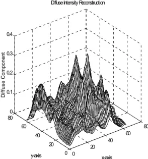
Figure 6 Reconstruction with Diffuse Component
Figure 7.Reconstruction with Specular Component
0 20
40 60
80
0 20 40 60 80
0 0.1 0.2 0.3 0.4
x-axis Diffuse Intensity Reconstruction
y-axis
D
if
fus
e C
om
ponent
0 5 10 15 20 25 30
228.2564 228.2566 228.2568 228.257 228.2572 228.2574 228.2576
no. of epoches
er
ror
Efficiency plot of training with ADAPTIVE learning
0 5 10 15 20 25 30 35 40 45 50 660.44
660.46 660.48 660.5 660.52 660.54 660.56 660.58
no. of epoches
e
rror
Figure 8. Reconstruction with Hybrid Component
V. CONCLUSION
In this paper a novel 3-D image reconstruction approach which considers both diffuse and specular components of the reflectance model simultaneously has been proposed. Two neural networks with symmetric structures were used to estimate these two components separately and to combine them with an adaptive ratio for each point on the object surface. This paper also attempted to reduce distortion caused by variable albedo variation by dividing each pixel’s intensity by corresponding albedo value. Then, these intensity values were fed into network to learn the normal vectors of surface by back-propagation learning algorithm. The parameters such as light source and viewing direction can be obtained from the neural network. The normal surface vectors thus obtained can then be applied to 3-D surface reconstruction by integration method.
REFERENCES
[1] Yuefang Gao, Jianzhong Cao, and Fei Luo, “A Hybrid-reflectance-modeled and Neural-network based Shape from Shading Algorithm”,
IEEE International Conference on Control and Automation Guangzhou, China - May 30 to June 1, 2007
[2] Wen-Chang Cheng,“Neural-Network-Based Photometric Stereo for 3D Surface Reconstruction,”2006 International Joint Conference on Neural Networks Sheraton Vancouver Wall Centre Hotel, Vancouver, BC, Canada July 16-21, 2006
[3] Chin-Teng Lin,Wen-Chang Cheng, and Sheng-Fu Liang, “
Neural-Network-Based Adaptive Hybrid-Reflectance Model for
3-D Surface Reconstruction, ” IEEE Transaction on Neural
Networks, Vol.16, No. 6, November 2005.
[4] Zhongquan Wu and Lingxiao Li, “A line-integration based method for depth recovery from surface normals”, IEEE Transactions on Pattern Analysis and Machine Intelligence, Vol.43, No.1, July 1988.
[5] S. Georghiades, P. N. Belhumeur, and D. J. Kriegman, “From few to many: illumination cone models for face recognition under variable lighting and pose,” IEEE Transactions on Pattern Analysis and Machine Intelligence, vol. 23, No.06, June 2001
Shalini Bhatia was born on August 08, 1971. She received the B.E. degree in Computer Engineering from Sri Sant Gajanan Maharaj
College of Engineering, Amravati University, Shegaon, Maharashtra, India in 1993, M.E. degree in Computer Engineering from Thadomal Shahani Engineering College, Mumbai, Maharashtra, India in 2003. She has been associated with Thadomal Shahani Engineering College since 1995, where she has worked as Lecturer in Computer Engineering Department from Jan 1995 to Dec 2004 and as Assistant Professor from Dec 2004 to Dec 2005. She has published a number of technical papers in National and International Conferences. She is a member of CSI and SIGAI which is a part of CSI.