www.biogeosciences.net/11/4507/2014/ doi:10.5194/bg-11-4507-2014
© Author(s) 2014. CC Attribution 3.0 License.
Low-level jets and above-canopy drainage as causes of turbulent
exchange in the nocturnal boundary layer
T. S. El-Madany1, H. F. Duarte2, D. J. Durden2,*, B. Paas1,**, M. J. Deventer1, J.-Y. Juang3, M. Y. Leclerc2, and O. Klemm1
1University of Münster, Climatology Working Group, Institute of Landscape Ecology, Münster, Germany 2The University of Georgia, Laboratory for Environmental Physics, Griffin, USA
3National Taiwan University, Department of Geography, Taipei, Taiwan *now at: NEON Inc., Boulder, USA
**now at: RWTH Aachen University, Physische Geographie und Klimatologie, Aachen, Germany
Correspondence to:T. S. El-Madany ([email protected])
Received: 24 January 2014 – Published in Biogeosciences Discuss.: 25 March 2014 Revised: 9 July 2014 – Accepted: 19 July 2014 – Published: 27 August 2014
Abstract. Sodar (SOund Detection And Ranging), eddy-covariance, and tower profile measurements of wind speed and carbon dioxide were performed during 17 consecutive nights in complex terrain in northern Taiwan. The scope of the study was to identify the causes for intermittent tur-bulence events and to analyze their importance in noctur-nal atmosphere–biosphere exchange as quantified with eddy-covariance measurements. If intermittency occurs frequently at a measurement site, then this process needs to be quanti-fied in order to achieve reliable values for ecosystem char-acteristics such as net ecosystem exchange or net primary production.
Fourteen events of intermittent turbulence were identified and classified into above-canopy drainage flows (ACDFs) and low-level jets (LLJs) according to the height of the wind speed maximum. Intermittent turbulence periods lasted between 30 and 110 min. Towards the end of LLJ or ACDF events, positive vertical wind velocities and, in some cases, upslope flows occurred, counteracting the general flow regime at nighttime. The observations suggest that the LLJs and ACDFs penetrate deep into the cold air pool in the val-ley, where they experience strong buoyancy due to density differences, resulting in either upslope flows or upward ver-tical winds.
Turbulence was found to be stronger and better developed during LLJs and ACDFs, with eddy-covariance data present-ing higher quality. This was particularly indicated by spectral analysis of the vertical wind velocity and the steady-state test
for the time series of the vertical wind velocity in combina-tion with the horizontal wind component, the temperature, and carbon dioxide.
Significantly higher fluxes of sensible heat, latent heat, and shear stress occurred during these periods. During LLJs and ACDFs, fluxes of sensible heat, latent heat, and CO2 were mostly one-directional. For example, exclusively negative sensible heat fluxes occurred while intermittent turbulence was present. Latent heat fluxes were mostly positive during LLJs and ACDFs, with a median value of 34 W m−2, while
outside these periods the median was 2 W m−2. In
conclu-sion, intermittent turbulence periods exhibit a strong impact on nocturnal energy and mass fluxes.
1 Introduction
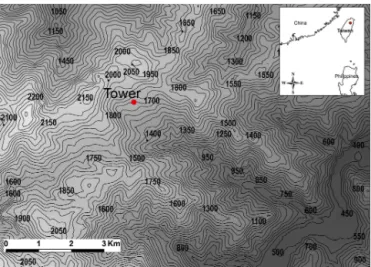
Figure 1.Topography of the experimental site and its surrounding. Numbers indicate the height above sea level (m) for the respective contour lines. The tower with the eddy-covariance and CO2profile measurements is indicated by a red dot. Light colors denote high elevation, and dark colors low elevations.
slopes in rather homogeneous terrain (Mahrt, 1999; Aubi-net, 2008), while gravity waves are usually caused by topo-graphic changes or irregularities of the canopy top (Lee et al., 1997). In complex terrain, all of these processes may occur, and a large effort has been made within projects like T-REX (T-REX stands for Terrain-induced Rotor EXperiment; Gru-bisic et al., 2008) and VTMX 2000 (Vertical Transport and MiXing; Doran et al., 2002) to understand the physics be-hind such (nocturnal) flows and how they influence transport of matter and energy (Cooper et al., 2006; Pinto et al., 2006; Reinecke and Durran, 2009; Choukulkar et al., 2012).
In cases of a stably stratified nocturnal boundary layer, tur-bulence is usually initialized by processes producing shear, e.g., drainage flows and gravity waves (Nakamura and Mahrt, 2005). This type of turbulence is referred to as intermittent turbulence or, as defined by Mahrt (1999), as global inter-mittency. This intermittent turbulence plays a major role in estimating nocturnal exchange of, e.g., CO2, but there is no consensus on how to treat longer time series when intermit-tent turbulence occurs at times. Variable data window sizes can lead to an increase of estimated turbulent energy and mass fluxes of 10 to 15 % (Acevedo et al., 2006). Mauder et al. (2013) address the difficulty to identify intermittency within eddy-covariance (EC) data sets.
In this study, an instrumental setup was deployed to iden-tify types of flow patterns that cause intermittent turbulence in complex terrain (Fig. 1). Preliminary studies at Chi-Lan Mountain (CLM), a site in northern Taiwan, showed that periods of strong intermittent turbulence may occur during the night. However, several questions could not be answered by using eddy-covariance data alone: (1) why does intermit-tency occur under various nocturnal situations? (2) Is the
in-termittency caused by drainage flows? (3) Are gusts or larger wind systems responsible for the intermittency?
To answer these questions, the present work combines wind profile measurements via sodar (SOund Detection And Ranging), near-surface turbulent flux measurements with the eddy-covariance method, and tower-based profile measure-ments of the CO2-concentration. Additionally, the influence of intermittent turbulence on turbulent nocturnal exchange above the forest will be estimated.
2 Measurements and data analysis 2.1 Site description
Eddy-covariance, sodar, and CO2profile measurements were performed at the CLM research site in northeastern Taiwan (24◦35′N, 121◦24′E). It is located in the upper part of a
val-ley at an elevation of 1650 m above sea level (Fig. 1) (Chang et al., 2002). The valley is orientated from northwest (top) to southeast (bottom) with an average slope of 14◦. The
vege-tation is dominated by a 50-year-old planvege-tation of Chamae-cyparis obtuse var. formosaandChamaecyparis formosensis
trees with an average canopy height between 11 and 14 m above ground (m a.g.). These coniferous trees have a plant area index (PAI) ranging from 2.75 m2m−2 in February to
5 m2m−2in September. During the experimental phase the
PAI was approximately 4 m2m−2. The wind system at CLM
is dominated by thermally driven daytime valley winds (from southeast) and nighttime mountain winds (from northwest) (Klemm et al., 2006; El-Madany et al., 2013). During the experiment, which was not within the typhoon season, no storms or strong precipitation events occurred. Especially during the nighttime, no precipitation occurred.
2.2 Instruments and setup
Two experimental towers were used in this study. One tower (T1) was equipped with two eddy-covariance systems and a profile system for CO2, the second tower (T2) was used to operate the sodar. Tower T2 was located at a distance of 20 m from T1 in the SSE direction.
The two eddy-covariance systems, each consisting of a R3-50 sonic anemometer (Gill Instruments, Ltd., Lymington, Hampshire, UK) for measuring the three-dimensional wind components as well as the sonic temperature and a LI-7500 (LI-COR Biosciences, Lincoln, Nebraska, USA) for measur-ing molar densities of CO2and H2O, were located at 5 and 10 m above the average canopy height (which corresponds to 19 and 24 m a.g.), respectively. Data were recorded and stored at 10 Hz sampling frequency.
of 15 m to all measuring levels. The sample air was pulled by an additional pump through the tubing. To prevent conden-sation water entering the gas analyzer, a water trap was in-stalled in front of the instrument. The sample flow rate of the gas analyzer was set to 0.5 L min−1and an automatic system
controlled the switching of the valves. Each level was sam-pled at the frequency of 1 Hz for 15 s, and the mean of the readings from the last 3 s for each level was collected. Sub-sequently, all measured values within a 30 min period were averaged to 30 min profiles.
A monostatic phased array Doppler sodar (model SFAS; Scintec AG, Rottenburg, Germany) was set up on T2 at 5 m above-canopy height (m a.c.) including a large enclosure (Scintec AG) to reduce the negative influence of ground clut-ter to the measurements, namely, a poor signal-to-noise ratio. After extensive testing, the following hardware and software configuration settings were used: the sodar antenna was lev-eled (vertical acoustic beam parallel to gravity) and orien-tated with a north offset of 100◦; a multi-frequency mode
was used to emit eight frequencies ranging from 3.059 to 4.843 kHz. Vertical profiles of the 3-D wind field between 10 and 305 m above the sodar antenna (25 to 320 m above ground) were calculated with a vertical resolution of 5 m and a temporal resolution of 10 min.
With this combination of local (eddy covariance and CO2 profiles) and remote sensing (sodar) techniques, the verti-cal structure of the wind and temporal evolution of turbulent fluxes can be investigated.
2.3 Data processing
Sensible heat, latent heat, momentum, and CO2 flux cal-culations were performed with EddyPro 4.1 (LI-COR Bio-sciences, Lincoln, Nebraska, USA) for each 30 min averag-ing period. Coordinate rotation was done with the planar fit method (Wilczak et al., 2001), linear detrending was used for trend removal, time lags were detected with covariance maxi-mization, WPL correction (Webb et al., 1980) was performed to compensate density fluctuation in the open-path gas ana-lyzer, and spectral corrections for high- and low-frequency loss were done according to Moncrieff et al. (1997) and Moncrieff et al. (in Lee et al., 2004), respectively. Quality checks were performed according to the Spoleto agreement, 2004, for CarboEurope IP (Mauder and Foken, 2011). The quality was determined by the stationarity of the time series and by the difference between the modeled integral turbu-lence characteristics (ITCs) and the measured ones (Foken and Wichura, 1996). Data sets that were not stationary and showed large differences between the modeled and the mea-sured integral turbulence characteristics were of quality class 2 and were not further used in this study.
A short-time Fourier transform was used to derive spec-tral characteristics of turbulence (i.e., vertical wind velocity) during jet periods. A Hemming window of 300 s length with 50 % overlap and a frequency band between 5 and 0.004 Hz
was used. This was short enough to achieve a good temporal resolution and long enough to capture small and medium size turbulence elements that contribute to the power spectral den-sity (PSD). Additionally, individual spectra were calculated for the vertical wind velocity before, during, and after the jet period. Depending on the length of the jet period, 214or 215 samples were taken, corresponding to∼27 and∼54 min, re-spectively.
The sodar data were processed with the APRun 1.43 soft-ware (Scintec AG). Raw data were averaged for 10 min in-tervals, and corrections such as ground clutter detection and removal were applied. For all cases in which data passed internal quality control (for further information see APRun Software Manual 2011), main data such as horizontal wind speed, wind components (u,v,w), wind direction, standard deviations of wind components (σu,σv,σw), and backscat-ter were calculated. Additional inbackscat-terpolation of missing data within the profiles was unnecessary due to the consistency of the data sets. Data gaps only occurred at the upper end of the measurement range and were left as they were.
Storage change fluxes of carbon dioxide were calcu-lated from profile measurements according to Aubinet et al. (2012), equation 1.24a term I.
2.4 Data selection
From 27 June to 14 July 2010, 17 nights (20:00–05:30 LT) were available for data analysis. Nighttime data were visually inspected to identify periods with LLJ activity and above-canopy drainage flows (ACDFs). From here on, the phrase “jet period” will be used for periods when either LLJ or ACDF occurred, while “no-jet period” will be used for the nocturnal data excluding jet periods.
LLJ events are defined as periods with a local wind speed maxima up to 270 m a.g. Higher low-level jets could not be clearly identified due to the upper limit of the sodar measure-ments (320 m a.g.). Additionally, these putative LLJs showed no influence on the wind field close to the canopy. They were therefore discarded from further analysis.
ACDFs are katabatic winds that are defined as periods in which the maximum horizontal wind speed within the lowest 100 m of the boundary layer occurred at the closest measure-ment level above the canopy (i.e., 5 m above the canopy).
To be included into further analysis, jet periods needed to last for at least 30 min so that they cover a full averaging period for the calculated fluxes.
Altogether, 14 events match the abovementioned criteria during the measurement period. They are listed in chrono-logical order with duration, height above ground of the wind speed maximum, maximum wind speed, and classification as LLJ or ACDF in Table 1.
Table 1.Fourteen jet periods during the experimental period with their duration, maximum wind speed, height of maximum wind speed, and the resulting classification as LLJ or ACDF.
Date Duration Max wind Height of max Classification (DD.MM) (hh:mm LT) speed (m s−1) wind speed (m)
27.06 00:30–01:00 3 Canopy ACDF
28.06 02:00–02:40 5 100 LLJ
29.06 04:40–05:40 6 130 LLJ
29.06–30.06 23:20–01:00 7 Canopy ACDF
01.07 00:40–01:10 3 100 LLJ
01.07 02:40–03:10 2 Canopy ACDF
03.07 20:30–22:20 11 180 LLJ
04.07 20:20–21:40 14 240 LLJ
07.07 04:00–04:30 4 Canopy ACDF
07.07 21:50–23:20 4 Canopy ACDF
08.07–09.07 23:10–00:30 7 100 LLJ
09.07 22:50–23:50 5 80 LLJ
11.07 00:20–02:10 6 90 LLJ
14.07 01:50–02:30 3 Canopy ACDF
Table 2.Percentiles of stability parameter (ζ), wind speed (m s−1), and TKE (turbulent kinetic energy in m2s−2)at height 5 and 10 m above
canopy for jet and no-jet periods.
Parameter Height ζ Wind speed TKE
Percentile 25th 50th 75th 25th 50th 75th 25th 50th 75th
No-jet period 5 0.092 0.212 0.356 1.09 1.54 1.95 0.174 0.232 0.349 Jet period 5 0.112 0.208 0.381 1.29 2.18 2.89 0.218 0.358 0.706
No-jet period 10 0.026 0.341 0.874 1.33 1.91 2.27 0.140 0.191 0.270 Jet period 10 0.278 0.615 0.942 1.63 2.23 2.83 0.187 0.311 0.624
considered as not affected. As mentioned above, only turbu-lent fluxes with quality classes 0 and 1 (Mauder and Foken, 2011) were used for the analysis of jet and no-jet periods.
3 Results
3.1 Atmospheric conditions
During the measurement period, eight low-level jets and six above-canopy drainage flows were identified. The durations of the events were between 30 and 110 min with a median of 60 min.
Before low-level jets or above-canopy drainage flows occurred, the horizontal wind speeds were usually be-low 0.5 m s−1 throughout the vertical profile. The Monin–
Obukhov stability parameter ζ, as calculated from sonic anemometer data, showed that typically weakly to moder-ately stable boundary layer conditions prevailed throughout all nights with jet periods. At 5 m a.c.,ζ was very similar for jet and no-jet periods, while at 10 m a.c. clearly higher val-ues ofζ occurred during jet periods (Table 2). Here, nearly
all situations were moderately stable while more than 25 % of the no-jet periods were weakly stable.
For both sonic anemometer measurement heights, the hor-izontal wind speed and turbulent kinetic energy (TKE) were higher for jet periods than for no-jet periods. A lower TKE at 10 m above canopy (m a.c.) as compared to 5 m a.c. indicates that nocturnal turbulence was mainly produced by the rough-ness of the canopy. This is true for both jet periods and no-jet periods. During no-no-jet periods, the horizontal wind speed was higher at 10 m a.c. as compared to 5 m a.c. while for jet periods no clear gradient was apparent. The missing gradi-ent was a result of analyzing LLJ and ACDF together. For LLJ and ADCF higher wind speeds are at 10 and 5 m a.c., respectively.
3.2 Low-level jets
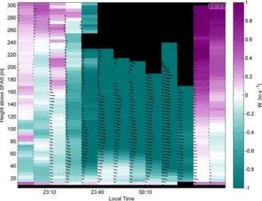
Figure 2 represents a typical LLJ of 80 min duration. Twenty minutes before the LLJ started, the lower part of the noc-turnal boundary layer (up to 250 m) was calm with wind speeds below 1 m s−1. During the LLJ maximum, horizontal
wind speeds of about 7 m s−1 occurred at altitudes between
Figure 2. Low-level jet event from 8 July at 22:50 LT to 9 July at 01:00 LT. Black arrows are wind vectors indicating wind speed (length) and wind direction (orientation). The width of one 10 min column corresponds to a wind speed of 11 m s−1. The vertical wind
speed is shown by the background colors. Positive vertical wind speeds are directed upwards, and negative wind speeds are directed downwards. The coordinate frame used is parallel to gravity (not normal to the surface). Positive vertical wind speeds are denoted with white to purple colors, while negative vertical wind speeds are white to teal. Wind speeds around zero are white. The time stamps and the beginning of the black arrows are located at the left side of the corresponding columns.
was WNW, and the vertical winds were clearly negative with speeds between−0.5 and−1.75 m s−1(parallel to gravity). The end of the LLJ was characterized by a sudden reduc-tion in horizontal wind speed. The horizontal wind speed dropped to maxima of about 0.5–1.0 m s−1 throughout the
profile, and the vertical wind speed became very small with values around zero up to 100 m above the sodar.
The termination of some jet periods was characterized by a change in wind direction of 180◦(from WNW to ESE) and
a reversal of the vertical wind component (Fig. 3). This cor-responded to an upward flow of the wind within the valley. This upward flow was not always as clearly pronounced as in this case (Fig. 3). In some cases the change of horizon-tal wind direction did not occur, but a reversal of the vertical wind component was apparent. After the upward flow, which typically lasted for 10 to 20 min, the jet period was over and wind speeds were small throughout the vertical profile.
3.3 Above-canopy drainage flows
A typical above-canopy drainage flow, as shown in Fig. 4, was characterized by a very pronounced maximum of wind speed just above the canopy. In this case (Fig. 4), the 30 min mean wind speed as measured by the sonic anemometer at 24 m a.g. was 3.0 and 3.6 m s−1 at 19 m a.g., respectively.
These measurements match well with the wind profile data
Figure 3. Same as Fig. 2 but from 28 June at 01:40–02:50 LT.
The width of one 10 min column corresponds to a wind speed of 5 m s−1.
measured by the sodar which showed a constant increase in the horizontal wind speed between 120 and 35 m above ground. The end of the drainage flow was characterized by a change in vertical wind speed from negative to positive, even though the wind direction was still from the northwest.
3.4 CO2profiles
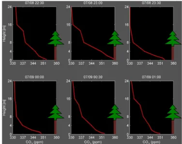
During the nights, when photosynthesis is absent, carbon dioxide typically accumulated at the surface of the forest as a result of nocturnal respiration of the soil and vegetation. Within the trunk space, the CO2mixing ratio decreased from the surface to the bottom of the canopy. Within the canopy it-self, the CO2mixing ratios were more or less constant, while above the canopy a further decrease with increasing altitude was apparent in all cases (Fig. 5).
During the LLJ of 8–9 July (Fig. 2; 23:30–01:30 LT), the CO2gradient between 0.5 and 24 m was reduced from 1.26 to 0.78 ppm m−1. The gradient between 24 and 8 m a.g. was
only 0.09 ppm m−1, indicating that the LLJ-induced
turbu-lence intruded into the canopy and led to strong mixing of the air above and inside the canopy. This mixing even affected the trunk space, and the near-surface mixing ratio dropped by 10 ppm. After termination of the LLJ, the gradient started to build up again. Sixty to ninety minutes later, the profile shape and the magnitude of the gradient were back to “nor-mal”, i.e., the conditions before onset of the LLJ.
Figure 4.Same as Fig. 3 but for an ACDF from 7 July at 03:40– 05:10 LT.
3.5 Turbulent exchange 3.5.1 Data quality
It was mentioned in Sect. 2.3 that data of quality class 2 were considered of minor quality in eddy covariance. The fraction of 30 min periods with this quality class varied strongly for the various fluxes. For example, for no-jet periods, the sen-sible heat and CO2fluxes exhibited 5 and 20 % higher frac-tions of quality class 2 data than for jet periods, respectively. In other words, jet period data were of better quality. The latent heat flux (LE) and shear stress (τ) were nearly of the same quality for no-jet and jet periods. Overall, latent heat flux data exhibited the least quality for no-jet and jet periods, with 36 % of the data being quality class 2.
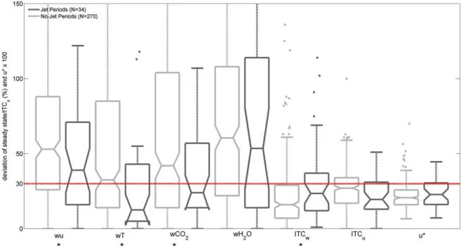
The percentile deviations from the steady-state condition for the time series ofwu,wT, andwCO2were significantly smaller for jet periods than for no-jet periods (Fig. 6). Far more data were below the 30 % threshold. According to Fo-ken (2008) and Mauder and FoFo-ken (2011), if deviations are below 30 % for the steady-state and ITC tests, the respective data sets fall into the best quality class. Consequently, this test also indicated a better quality for jet periods as compared to no-jet periods.
For no-jet periods the ITCw deviations were significantly smaller than for jet periods. Nevertheless, more than 50 % of the ITCw values were smaller than the 30 % threshold for jet periods. For ITCu, all quartile values were smaller under jet periods, but the difference was not significant (Fig. 6). All quartile values ofu∗were smaller for no-jet periods as
compared to jet periods. It can be stated that more turbulence was present during jet periods. For reliable eddy-covariance measurements at night, a minimum of turbulence is required. As described by Goulden et al. (1996), the friction velocity (u∗) should be larger than 0.17 m s−1. According to Barr et
Figure 5.Thirty minute averaged CO2 profiles from 8 measure-ment heights from 8 July at 22:30 LT to 9 July at 01:00 LT. The tree scheme indicates the location of the canopy and the trunk space with respect to the profile measurement points. The 23:30 LT and the 00:00 LT profiles are during the LLJ of Fig. 2. The time stamps indicate the beginning of the 30 min averaging period for the re-spective profiles.
al. (2013) each site has a specificu∗ threshold value.
Nev-ertheless, the value of 0.17 m s−1was taken as a rough
es-timate. For both jet and no-jet periods, 75 % of the data ex-ceeded this threshold. Theu∗values during jet periods were
clearly higher, and therefore eddy-covariance data tended to be of better quality.
3.5.2 Spectral characteristics
Figure 6.Box plots of percentile deviation of steady state for time series of vertical wind velocity with streamwise wind velocity, temperature,
CO2and H2O (wu,wT,wCO2,wH2O) as well as percentile deviations of measured integral turbulence characteristics from modeled values for vertical and streamwise wind velocity (ITCw, ITCu), and the friction velocity (u∗), multiplied by 100 to fit the scale. Box plots for no-jet periods are plotted in light grey, while jet periods are plotted in dark grey. Stars denote significant differences between jet and no-jet periods. The red line at the value of 30 represents the thresholds for the best quality class. It represents a 30 % deviation of the ITC and steady-state criteria as well as a friction velocity of 0.3 m s−1. The whiskers are set to 1.5 interquartile range, and the boxes are waisted to accentuate the
median value.
3.5.3 Fluxes
Flux data as presented here were of quality class 1 and 0, ex-clusively. Fluxes of sensible heat and latent heat were of sig-nificantly larger magnitude during jet periods as compared to no-jet periods (Fig. 8). During no-jet periods, the median of latent heat fluxes was close to 0, and the first and third quar-tiles were at−18 and+21 Wm−2(upper EC), respectively. For jet periods, latent heat fluxes were clearly positive with first and third quartiles of 9 W m−2 and 58 W m−2 (upper
EC). The direction of the fluxes was positive and therefore directed from the vegetation into the atmosphere. During no-jet periods, sensible heat fluxes were mostly negative, while for jet periods they were only negative and of larger magni-tude (Fig. 8). Only for the upper EC system did a significant difference occur between CO2fluxes during no-jet periods and jet periods. Nevertheless, more positive fluxes occurred during jet periods, and all quartile values were higher or less negative for the upper and the lower EC systems. For sensi-ble heat flux, latent heat flux, and the CO2flux, no signif-icant differences occurred between the upper and the lower EC systems during jet periods and no-jet periods (Fig. 8). Only for shear stress were significant differences observed between the upper and the lower EC system during jet peri-ods and no-jet periperi-ods.
The lower EC system measured significantly higher shear stress under jet periods and no-jet periods as compared to the upper EC system.
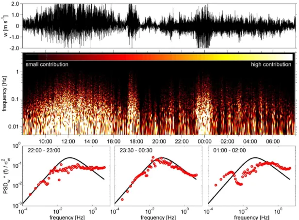
Figure 7.Top panel: 24 h time series of 10 Hz vertical wind velocity data as measured with the sonic anemometer at 10 m above canopy. Middle panel: spectrogram of the vertical wind velocity data from the top panel. Dark colors indicate frequencies with small contributions to power spectral density (m s−2), while light colors indicate high contributions from the respective frequencies. Bottom panel: normalized
power spectral density of the vertical wind velocity (red circles) and the respective model spectrum (solid black line) according to Rannik and Vesala (2006). Left and right panel represent spectra of 60 min periods before and after the jet period, respectively. The middle panel is the 60 min spectrum of the vertical wind velocity during the jet period.
4 Discussion
4.1 Origin of low-level jets and above-canopy drainage flows
No information about the development of LLJ and ACDF or their driving processes can be deducted from the employed experimental setup. Nevertheless, it is clear that the initia-tion of the LLJ and ACDF must be upslope of the instrumen-tal setup because the wind direction was northwest for all observed jet periods.
The data clearly show that jet periods occurred under mod-erately stable to very stable boundary layer conditions with low horizontal wind speeds throughout the vertical profile (Figs. 2–4 and Table 2). Such situations favor the formation of katabatic winds (i.e., ACDF), especially when the synop-tic forcing is small (Zangl, 2009). When decoupling between the surface layer and air aloft occurs, the development of a LLJ is likely (Stull, 1988). According to Mahrt (1999), cool-ing over sloped terrain leads to a time-dependent and height-dependent horizontal pressure-gradient force that sets con-ditions favorable for the development of the LLJ.
Remark-ably, all observed LLJ and ACDF follow the orientation of the valley and flow downward from northwest to southeast (Figs. 2–4). This is typical for a katabatic wind that occurs at the surface and has to follow the terrain in a valley. For LLJ this implies that the decoupling between the surface layer and the air above where the LLJ forms – e.g., at the top of an in-version – follows the valley slope.
Jet periods show continuous and well-developed turbu-lence throughout wide frequency scales from their sud-den beginning until their likewise sudsud-den ending (Fig. 7 23:30–00:30 LT). Assuming that the initiation of the jet pe-riod is between the mountain ridge and the location of the tower, and assuming that it is initialized from a non-turbulent situation, the turbulence must have development along a roughly 1000 m long path with a steep slope of 17–21◦
Figure 8.Box plots of sensible heat flux (W m−2), latent heat flux (W m−2), CO
2flux (µmol m−2s−1), and shear stress (kg m−1s−2)for the upper and the lower eddy-covariance setups during jet periods and no-jet periods. CO2flux values were multiplied by 10 and shear stress values by 500 to fit the scale. Capital letters on thexaxis denote significant differences between the upper and the lower EC during no-jet periods(a)and during jet periods(b)as well as differences between jet periods and no-jet periods for the upper EC(c)and the lower EC(d).
The whiskers are set to 1.5 interquartile range, and the boxes are waisted to accentuate the median value.
Since the mountain ridge is located upwind of the mea-surement site, it is highly likely that the jet periods are caused by local processes such as surface cooling (e.g., katabatic flows such as ACDF), topographic effects such as mountain waves that initiate katabatic flows (Banta et al., 2004), and a terrain that is favorable or adverse for building up pressure gradients. Larger-scale synoptic forcing, such as the propaga-tion of a front as described by Sheridan and Vosper (2012), is not likely to have occurred because synoptic-scale pres-sure gradients are rather small and the frontal approach, as generally applied in the high latitudes, does not apply in the tropics and subtropics (Riehl, 1954).
4.2 Jet periods and turbulent exchange
The nocturnal turbulent exchange depends mostly on atmo-spheric conditions such as wind speed and atmoatmo-spheric sta-bility. During strongly stable conditions the turbulence is very weak and not well developed, and therefore the fluxes are small and the CO2 accumulates near the surface. This is apparent from CO2 profiles (Fig. 5); vertical wind
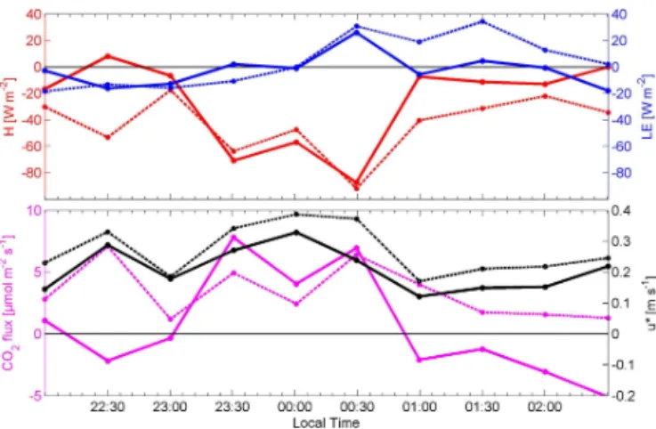
Figure 9.Fluxes of sensible heat (H, red), latent heat (LE, blue), CO2(magenta), and friction velocity (u∗, black) for the LLJ from
8 July at 23:30 LT to 9 July at 00:30 LT (Fig. 2). Dashed lines with markers represent fluxes from the lower EC system and solid lines with markers represent fluxes from the upper EC system. Straight solid lines indicate zero lines of the respective variables.
the jet period, SCFs changed their direction, with values be-tween 1.0 and 4.0 µmol m−2s−1. These positive SCFs were
most likely caused by a combination of respiration of the soil and plants as well as sub-canopy drainage with CO2-enriched air. The drainage flows could explain the large fluctuations of the SCFs after jet periods and during the no-jet periods.
As compared to no-jet periods, the sensible heat fluxes during jet periods were frequently more negative and of larger magnitude (Figs. 8 and 9). Strong surface cooling dur-ing the night led to temperature inversions. As shown in Wolfelmaier et al. (1999), LLJ and katabatic flows are likely to occur at the top of temperature inversions in complex ter-rain. The resulting turbulence mixed warm air from above and cold air from the canopy surface. This led to exclu-sively negative and strong sensible heat fluxes (Figs. 8 and 9). The results also indicate a temporal increase in air tem-perature (data not shown) which match the findings of Pinto et al. (2006) from T-REX.
4.3 Duration and ending of jet periods
The longest jet period observed in this study lasted for 110 min and was a LLJ. These were rather short time periods in comparison to those observed at other sites, especially flat terrain sites, where a LLJ can last throughout the night until the beginning of dawn (e.g., Whiteman et al., 1997; Banta et al., 2007; Duarte et al., 2012). On the other hand, the shortest duration of a jet period (30 min) was too long to be explained only by the occurrence of gusts (Acevedo et al., 2006), and the vertical wind profiles provided no indication of gusts dur-ing jet periods. Results of Pinto et al. (2006) and Chiao and Dumais (2013) from the VTMX and T-REX project, respec-tively, showed longer duration and larger depth of the de-tected jets on a larger topographic scale. The CLM valley is
Figure 10.Scheme of the above-canopy drainage (top) and the re-spective counter flows (middle and bottom) at the end of the ACDF. Color scale indicates temperatures ranging from cooler tempera-tures (blue) to warmer temperatempera-tures (red). Arrows show the wind direction. Black surface represents the slope of the valley.
roughly 2 km wide and 8 km long (Fig. 1), while the Great Salt Lake Valley and Owens Valley (where VTMX and T-REX were performed) are much larger (about 5 to 10 times). This indicates that jets can occur on various spatial scales and that their duration is dependent on the size of the valley.
CLM are located at the upper part of the valley (Fig. 1). Due to the structure of the valley and the unrestricted outflow of cold air, it is very unlikely that the cold pool ever reaches the towers (Fig. 1). Therefore, such conditions are very unlikely to be the cause of the termination of the jet periods.
A process that is retrieved from large eddy simulation results, and which is described by Zhou and Chow (2012, 2013), offers an explanation for the observed uphill flows at the end of the jet periods: surface cooling leads to a kata-batic flow (Fig. 10, top panel). The air flows down the valley until it reaches the height of neutral buoyancy. If the momen-tum of the katabatic flow is high, it overshoots the height of neutral buoyancy and dives into air masses of lower tempera-tures and higher density. At this point, it experiences positive buoyancy and flows upwards until it reaches the point of neu-tral buoyancy again. Such counter flows may either maintain their horizontal wind direction and only change the direc-tion of the vertical wind component (Fig. 10, middle panel) or change horizontal wind direction and the direction of the vertical wind component, which results in an upslope flow (Fig. 10, bottom panel).
At the Chi-Lan Mountain site, both LLJ and ACDF fol-low the terrain downhill; therefore it is possible for both to overshoot the point of neutral buoyancy in the described way. Depending on the stratification of the boundary layer and the strength of the jet period, both a vertical air motion (Figs. 2, 4) and an uphill flow (Fig. 3) may establish the state of equi-librium.
5 Conclusions
With the use of a sodar with high vertical resolution (5 m) and a vertical range of 300 m, it was possible to identify two types of nocturnal flows that cause intermittent turbulence in complex terrain. With the help of two eddy-covariance se-tups, employed as an extension of the vertical wind profile of the sodar, a clear distinction between LLJ and ACDF was possible. Effects of LLJ and ACDF on turbulent exchange processes and data quality could be quantified and shown to be very similar for both cases.
The causes and driving processes for LLJ and ADCF pe-riods could not be completely clarified, but a stable stratifi-cation and the terrain of the valley play major roles. Gusts or large-scale wind systems could be excluded as sources.
Profile measurements of CO2 concentration clearly showed that strong CO2 fluxes during the jet periods are caused by a decay of a CO2pool that had accumulated dur-ing calm conditions before the jet period. Nocturnal LLJ and ACDF can lead to a coupling of above-canopy and below-canopy air and therefore result in strong fluxes of mass and energy. Due to their frequent occurrence, jet periods play a major role for the nocturnal turbulent exchange at CLM.
It is evident from the presented data that jet periods lead to canopy exchange processes that are considerably different
from those during their absence. Although eddy-covariance data quality during no-jet periods is lower than during jet pe-riods, which makes a comparison of the fluxes difficult, it is evident that fluxes are generally smaller in the absence of LLJs and ACDFs. For sites with frequent occurrence of inter-mittent turbulence, these differences between jet and no-jet periods should be taken into account. Therefore, long-term data sets should be analyzed carefully to avoid any overesti-mate of nocturnal fluxes due to gap-filling algorithms or to flagging high flux data during quality control.
This work provided measurements of upslope moving air in nocturnal stable boundary layer conditions. This phe-nomenon occurred for only about 10 to 20 min at the end of LLJ and ACDF events. It appears to be caused by an over-shooting of LLJ or ACDF below the point of neutral buoy-ancy and the respective equalization during which air can flow upslope.
Further studies incorporating scanning lidars and micro-barographs could provide more insight into the development of LLJs and ACDFs, their driving processes, and the roles of gravity waves in this context.
Acknowledgements. This work was supported by the Deutsche Forschungsgemeinschaft (DFG) through project KL623/10-1. The authors thank Niels Thiermann from Scintec, Shih-Chieh Chang, Shih-Bin Ding, Natchaya Pingintha, and Pei-Ling for the great support of our fieldwork at CLM.
Edited by: K. Jardine
References
Acevedo, O. C., Moraes, O. L. L., Degrazia, G. A., and Medeiros, L. E.: Intermittency and the exchange of scalars in the nocturnal surface layer, Bound.-Lay. Meteorol., 119, 41–55, 2006. Aubinet, M.: Eddy covariance CO2flux measurements in nocturnal
conditions: An analysis of the problem, Ecol. Appl., 18, 1368– 1378, 2008.
Aubinet, M., Berbigier, P., Bernhofer, C. H., Cescatti, A., Feigen-winter, C., Granier, A., Grunwald, T. H., Havrankova, K., Heinesch, B., Longdoz, B., Marcolla, B., Montagnani, L., and Sedlak, P.: Comparing co2 storage and advection conditions at night at different carboeuroflux sites, Bound.-Lay. Meteorol., 116, 63–94, 2005.
Aubinet, M., Vesala, T., and Papale, D.: Eddy covariance – a prac-tical guide to measurement and data analysis, Springer, 2012. Banta, R. M., Newsom, R. K., Lundquist, J. K., Pichugina, Y. L.,
Coulter, R. L., and Mahrt, L.: Nocturnal low-level jet character-istics over kansas during cases-99, Bound.-Lay. Meteorol., 105, 221–252, 2002.
Banta, R. M., Darby, L. S., Fast, J. D., Pinto, J. O., Whiteman, C. D., Shaw, W. J., and Orr, B. W.: Nocturnal low-level jet in a moun-tain basin complex – Part I: Evolution and effects on local flows, J.Appl. Meteorol., 43, 1348–1365, 2004.
nights with weak low-level jets, J. Atmos. Sci., 64, 3068–3090, 2007.
Barr, A. G., Richardson, A. D., Hollinger, D. Y., Papale, D., Arain, M. A., Black, T. A., Bohrer, G., Dragoni, D., Fischer, M. L., Gu, L., Law, B. E., Margolis, H. A., McCaughey, J. H., Munger, J. W., Oechel, W., and Schaeffer, K.: Use of change-point detection for friction-velocity threshold evaluation in eddy-covariance studies, Agr. For. Meteorol., 171, 31–45, 2013.
Belcher, S. E., Finnigan, J. J., and Harman, I. N.: Flows through forest canopies in complex terrain, Ecol. Appl., 18, 1436–1453, 2008.
Chang, S. C., Lai, I. L., and Wu, J. T.: Estimation of fog deposition on epiphytic bryophytes in a subtropical montane forest ecosys-tem in northeastern taiwan, Atmos. Res., 64, 159–167, 2002. Chiao, S. and Dumais, R.: A down-valley low-level jet event during
t-rex 2006, Meteorol. Atmos. Phys., 122, 75–90, 2013.
Choukulkar, A., Calhoun, R., Billings, B., and Doyle, J.: Investi-gation of a complex nocturnal flow in owens valley, california using coherent doppler lidar, Bound.-Lay. Meteorol., 144, 359– 378, 2012.
Cooper, D. I., Leclerc, M. Y., Archuleta, J., Coulter, R., Eichinger, W. E., Kao, C. Y. J., and Nappo, C. J.: Mass exchange in the stable boundary layer by coherent structures, Agr. For. Meteorol., 136, 114–131, 2006.
Darby, L. S., Allwine, K. J., and Banta, R. M.: Nocturnal low-level jet in a mountain basin complex. Part ii: Transport and diffusion of tracer under stable conditions, J. Appl. Meteorol. Climatol., 45, 740–753, 2006.
Doran, J. C., Fast, J. D., and Horel, J.: The vtmx 2000 campaign, Bull. Am. Meteorol. Soc., 83, 537–551, 2002.
Duarte, H. F., Leclerc, M. Y., and Zhang, G. S.: Assessing the shear-sheltering theory applied to low-level jets in the nocturnal stable boundary layer, Theoret. Appl. Climatol., 110, 359–371, 2012. Durden, D. J., Nappo, C. J., Leclerc, M. Y., Duarte, H. F., Zhang,
G., Parker, M. J., and Kurzeja, R. J.: On the impact of wave-like disturbances on turbulent fluxes and turbulence statistics in nighttime conditions: A case study, Biogeosciences, 10, 8433– 8443, doi:10.5194/bg-10-8433-2013, 2013.
El-Madany, T. S., Griessbaum, F., Fratini, G., Juang, J. Y., Chang, S. C., and Klemm, O.: Comparison of sonic anemometer perfor-mance under foggy conditions, Agr. For. Meteorol., 173, 63–73, 2013.
Foken, T.: Micrometeorology, Springer, Berlin and Heidelberg, 328 pp., 2008.
Foken, T. and Wichura, B.: Tools for quality assessment of surface-based flux measurements, Agr. Forest Meteorol., 78, 83–105, 1996.
Goulden, M. L., Munger, J. W., Fan, S. M., Daube, B. C., and Wofsy, S. C.: Measurements of carbon sequestration by long-term eddy covariance: Methods and a critical evaluation of accuracy, Glob. Change Biol., 2, 169–182, 1996.
Grubisic, V., Doyle, J. D., Kuettner, J., Mobbs, S., Smith, R. B., Whiteman, C. D., Dirks, R., Czyzyk, S., Cohn, S. A., Vosper, S., Weissmann, M., Haimov, S., De Wekker, S. F. J., Pan, L. L., and Chow, F. K.: The terrain-induced rotor experiment a field cam-paign overview including observational highlights, Bull. Am. Meteorol. Soc., 89, 1513–1533, 2008.
Huang, J. and Bou-Zeid, E.: Turbulence and vertical fluxes in the stable atmospheric boundary layer. Part i: A large-eddy simula-tion study, J. Atmos. Sci., 70, 1513–1527, 2013.
Karipot, A., Leclerc, M. Y., Zhang, G. S., Lewin, K. F., Nagy, J., Hendrey, G. R., and Starr, G.: Influence of nocturnal low-level jet on turbulence structure and co2 flux measurements over a forest canopy, J. Geophys. Res.-Atmos., 113, D10102, doi:10.1029/2007jd009149, 2008.
Klemm, O., Chang, S. C., and Hsia, Y.: Energy fluxes at a subtropi-cal mountain cloud forest, For. Ecol. Manag., 224, 5–10, 2006. Kutsch, W. L., Kolle, O., Rebmann, C., Knohl, A., Ziegler, W., and
Schulze, E. D.: Advection and resulting CO2exchange uncer-tainty in a tall forest in central germany, Ecol. Appl., 18, 1391– 1405, 2008.
Lee, X., Neumann, H. H., DenHartog, G., Fuentes, J. D., Black, T. A., Mickle, R. E., Yang, P. C., and Blanken, P. D.: Observation of gravity waves in a boreal forest, Bound.-Lay. Meteorol., 84, 383–398, 1997.
Lee, X., Massman, W., and Law, B.: Handbook of micrometeorol-ogy – a guide for surface flux measurement and analysis, Kluwer Academic Press, Dordrecht, 250 pp., 2004.
Lee, X. H.: A model for scalar advection inside canopies and appli-cation to footprint investigation, Agr. For. Meteorol., 127, 131– 141, 2004.
Mahrt, L.: Stratified atmospheric boundary layers, Bound.-Lay. Me-teorol., 90, 375–396, 1999.
Mahrt, L.: Computing turbulent fluxes near the surface: Needed im-provements, Agr. For. Meteorol., 150, 501–509, 2010.
Mahrt, L., Richardson, S., Seaman, N., and Stauffer, D.: Non-stationary drainage flows and motions in the cold pool, Tellus A, 62, 698–705, 2010.
Mathieu, N., Strachan, I. B., Leclerc, M. Y., Karipot, A., and Pattey, E.: Role of low-level jets and boundary-layer properties on the nbl budget technique, Agr. For. Meteorol., 135, 35–43, 2005. Mauder, M. and Foken, T.: Dokumentation and instruction
man-ual of the eddy-covariance software package tk3, Universität bayreuth, Abteilung Mikrometeorologie, Arbeitsergebnisse, 46, 2011.
Mauder, M., Cuntz, M., Drüe, C., Graf, A., Rebmann, C., Schmid, H. P., Schmidt, M., and Steinbrecher, R.: A strategy for quality and uncertainty assessment of long-term eddy-covariance measurements, Agr. For. Meteorol., 169, 122–135, 2013. Moncrieff, J. B., Massheder, J. M., deBruin, H., Elbers, J.,
Fri-borg, T., Heusinkveld, B., Kabat, P., Scott, S., Soegaard, H., and Verhoef, A.: A system to measure surface fluxes of momentum, sensible heat, water vapour and carbon dioxide, J. Hydrol., 189, 589–611, 1997.
Nakamura, R. and Mahrt, L.: A study of intermittent turbulence with cases-99 tower measurements, Bound.-Lay. Meteorol., 114, 367–387, 2005.
Oliveira, P. E. S., Acevedo, O. C., Moraes, O. L. L., Zimermann, H. R., and Teichrieb, C.: Nocturnal intermittent coupling between the interior of a pine forest and the air above it, Bound.-Lay. Me-teorol., 146, 45–64, 2013.
Reinecke, P. A. and Durran, D. R.: Initial-condition sensitivities and the predictability of downslope winds, J. Atmos. Sci., 66, 3401– 3418, 2009.
Riehl, H.: Tropical meteorology, McGraw-Hill, New York„ 392 pp., 1954.
Sheridan, P., and Vosper, S.: High-resolution simulations of lee waves and downs lope winds over the sierra nevada during T-REX iop 6, J. Appl. Meteorol. Climatol., 51, 1333–1352, 2012. Stull, R. B.: An introduction to boundary layer meteorology,
Kluwer Academic Publishers, Dordrecht, Boston, London, 666 pp., 1988.
Sun, J. L., Mahrt, L., Banta, R. M., and Pichugina, Y. L.: Turbulence regimes and turbulence intermittency in the stable boundary layer during cases-99, J. Atmos. Sci., 69, 338–351, 2012.
Vecenaj, Z., De Wekker, S. F. J., and Grubisic, V.: Near-surface characteristics of the turbulence structure during a mountain-wave event, J. Appl. Meteorol. Climatol., 50, 1088–1106, 2011. Webb, E. K., Pearman, G. I., and Leuning, R.: Correction of flux
measurements for density effects due to heat and water-vapor transfer, Quart. J. Roy. Meteorol. Soc., 106, 85–100, 1980. Whiteman, C. D., Bian, X. D., and Zhong, S. Y.: Low-level jet
cli-matology from enhanced rawinsonde observations at a site in the southern great plains, J. Appl. Meteorol., 36, 1363–1376, 1997.
Wilczak, J. M., Oncley, S. P., and Stage, S. A.: Sonic anemometer tilt correction algorithms, Bound.-Lay. Meteorol., 99, 127–150, 2001.
Wolfelmaier, F. A., King, C. W., Mursch-Radlgruber, E., and Ren-garajan, G.: Mini-sodar observations of drainage flows in the rocky mountains, Theoret. Appl. Climatol., 64, 83–91, 1999. Zangl, G.: The impact of weak synoptic forcing on the valley-wind
circulation in the alpine inn valley, Meteorol. Atmos. Phys., 105, 37–53, 2009.
Zeri, M. and Sa, L. D. A.: Horizontal and vertical turbulent fluxes forced by a gravity wave event in the nocturnal atmospheric sur-face layer over the amazon forest, Bound.-Lay. Meteorol., 138, 413–431, 2011.
Zhou, B. and Chow, F. K.: Nighttime cold-air intrusions and tran-sient warming in a steep valley: A nested large-eddy simula-tion study, 15th Conference on Mountain Meteorology 08/19/– 08/24/2012, Steamboat Springs, Colorado, 2012.
Zhou, B. W. and Chow, F. K.: Nested large-eddy simulations of the intermittently turbulent stable atmospheric boundary layer over real terrain, J. Atmos. Sci., 70, 3262–3276, 2013.